Discovery, Photometry, and Kinematics of Planetary Nebulae in M 82

Abstract

Using an [O iii] $\lambda$5007 on-band/off-band filter technique, we identify 109 planetary nebulae (PNe) candidates in the edge-on spiral galaxy M 82, using the FOCAS instrument at the 8.2m Subaru Telescope. The use of ancillary high-resolution Hubble Space Telescope ACS H$\alpha$ imaging aided in confirming these candidates, helping to discriminate PNe from contaminants such as supernova remnants (SNRs) and compact Hii regions. Once identified, these PNe reveal a great deal about the host galaxy; our analysis covers kinematics, stellar distribution, and distance determination. Radial velocities were determined for 94 of these PNe using a method of slitless spectroscopy, from which we obtain a clear picture of the galaxy’s rotation. Overall, our results agree with those derived by CO(2-1) and Hi measurements (Sofue 1998) that show a falling, near-Keplerian rotation curve. However, we find a subset of our PNe that appear to lie far ($\sim 1$ kpc) above the plane, yet these objects appear to be rotating as fast as objects close to the plane. These objects will require further study to determine if they are members of a halo population, or if they can be interpreted as a manifestation of a thickened disk as a consequence of a past interaction with M 81. In addition, [O iii] $\lambda$5007 emission line photometry of the PNe allows the construction of a planetary nebula luminosity function (PNLF) for the galaxy. Our distance determination for M 82, deduced from the observed PNLF, yields a larger distance than those derived using the tip of the red giant branch technique (TRGB; Dalcanton et al. 2009), using Cepheid variable stars in nearby group member M 81 (Freedman et al. 1994), or using the PNLF of M 81 (Jacoby et al. 1989). We show that this inconsistency most likely stems from our inability to completely correct for internal extinction imparted by this dusty, starburst galaxy. Additional observations that yield object-by-object foreground and internal extinction corrections are required to make an accurate distance measurement to this galaxy.

1. Introduction

Studies of extragalactic planetary nebulae (PNe) have successfully contributed to astronomy in a number of different ways. The use of the planetary nebulae luminosity function (PNLF) as a distance indicator (see e.g. Jacoby et al. 1989) has achieved remarkable success (Ciardullo 2003). Extragalactic PNe have been used to study galaxy cluster evolution and intracluster stellar populations in the Virgo cluster (Feldmeier et al. 2004; Arnaboldi et al. 2008). The fact that accurate radial velocities can be obtained from these PNe, once they are discovered, has made them increasingly important as kinematic probes in the outskirts of galaxies. A classic example is the study of PNe in NGC 5128 by Hui et al. (1995); they found evidence of dark matter around this elliptical galaxy, as expected from the currently favored scheme for galaxy formation. This finding put forth the notion that further PN searches could lead to the accumulation of evidence supporting the ubiquity of dark matter in elliptical galaxies, as convincing as in the case of spiral galaxies. However, discussion continues in the confusing case of “ordinary” or “average” ellipticals, where PNe show little apparent influence from dark matter halos. While the case for “no dark matter” is weakening as the effect of radial anisotropy on PN orbits is better understood, recent studies by De Lorenzi et al. (2008), Méndez et al. (2009), and Napolitano et al. (2009) show that clarification to this confusing situation will only come from further observations in elliptical galaxies. The fact is clear, however, that PNe act as versatile probes for studies of extragalactic astronomy.

In this paper we explore possible uses for PNe in the nearly edge-on, starburst spiral galaxy M 82. To our knowledge no PN search in this galaxy has been tried up to now, probably because a large amount of dust and internal extinction makes it very difficult to attempt a PNLF distance determination.

M 82 is relatively nearby (3.55 Mpc; Dalcanton et al. 2009), making it a prime target for extragalactic PN identifications. Its archetypal starburst activity and high infrared luminosity have induced many studies, giving us the added benefit of the availability of an assortment of existing multi-wavelength observations. This peculiar edge-on galaxy has been found to have both a central bar (Telesco et al. 1991; Achtermann & Lacy 1995) and the signature of spiral arms (Mayya, Carrasco, & Luna 2005). Sofue et al. (1992) presented CO data that showed a rotation curve for the galaxy that declined in nearly Keplerian fashion, making this system a unique example of a spiral galaxy that shows little apparent influence from dark matter. Sofue (1998) goes on to suggest that the peculiar rotation shown in CO and Hi data (Yun, Ho, & Lo 1993) may be the result of an interaction with M 81 several hundred Myr ago. Evidence of a galactic interaction exists in the form of a Hi bridge and streamers connecting M 81, M 82, and NGC 3077 (Cottrell 1977; Yun, Ho, & Lo 1994), and such features were successfully reproduced in a numerical model of the encounter presented by Yun (1999).

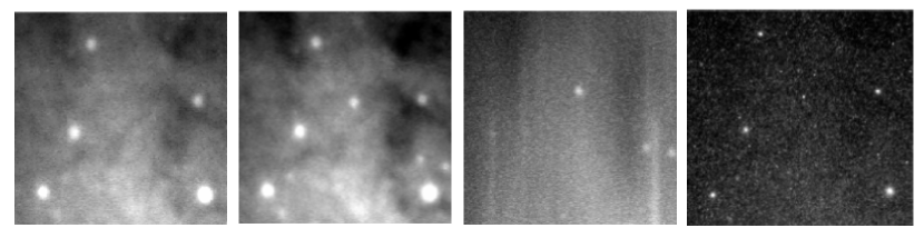
Figure 1.— Image subsections taken from final stacked images. From left to right: FOCAS off-band, on-band, and grism (on-band + grism) image subsections; at the extreme right, HST H$\alpha$ image subsection (see Section 3.2). Subsections shown are each $20^{\prime\prime}\!\!\times 20^{\prime\prime}\!\!$. Three PN candidates are present in the on-band frame and can be identified by their absence in the off-band frame. The PN candidates appear again as point sources in the grism frame, shifted upwards in the direction of dispersion. The displacement distance is a function of wavelength of the PN emission feature, which in turn provides the object’s radial velocity. The high-resolution HST image has superior ability to resolve non-PN objects and detect source extension.

Our initial focus was to test the accuracy of the slitless radial velocity method on a well-studied target and to confirm the ability of PNe to reproduce the behavior of a kinematically well-known population. As spiral galaxies show distinctive kinematic qualities, such as a well-defined rotation curve, M 82 makes a good test object. However, when we observed large numbers of PNe at great heights from the galactic plane, the emphasis shifted toward exploring the distribution and kinematic behavior of the stellar population that is producing the detected PNe. We also wish to explore how reliable a PNLF distance determination is in a difficult case like this.

In § 2 we describe the technique for the detection of PNe, explain the method of slitless spectroscopy for determining radial velocities, and introduce the PNLF. We discuss observations and image reductions in § 3, followed by a consideration of PN identifications and selection criteria in § 4. Radial velocity determination methods and results, as well as a discussion of means for validating our findings, are presented in § 5. Photometry, PNLF fitting, and our distance measurement are considered in § 6. We close in § 7 with a summary.

2. Planetary Nebulae, Slitless Spectroscopy, and the PNLF

The spectra of PNe characteristically show a very strong [O iii] $\lambda$5007 nebular emission line due to the excitation of a metastable level in a ground configuration by collisions with electrons. The colliding electrons are the result of ionization of low-density gas by extremely diluted UV photons from the PN central star. Due to the presence of this very strong [O iii] emission, PNe are easily detected using an on-band/off-band technique which involves blinking images taken through suitable on-band and off-band filters. As shown in the first and second frames of Figure 1, while normal stars appear in both images, PNe can be identified by their differential appearance: absent in the off-band image, yet present in the on-band image. Off-band images are exposed to a deeper limiting magnitude than the corresponding on-band image in order to ensure the validity of the non-detection.

An additional technique to substantiate the detection of a PN makes use of an on-band, grism-dispersed image. This image is taken directly following the on-band image; the telescope continues tracking and the observing system is left unchanged between exposures, with exception to the addition of a dispersing grism placed into the light path. In this configuration, the continuum light of a star will be shifted and dispersed into a segment of light on the image, whose length is determined by the bandpass of the filter used. However, a PN will appear as a shifted point source, due to the nearly monochromatic nature of its emission. The third panel of Figure 1 clearly shows that the three PN candidates detected by comparing the on-band and off-band images indeed appear as point sources on the grism image.

The power of the grism image not only lies in its ability to aid PN identification, but also in its ability to provide velocity data for each source. The shift in position that occurs when we insert the grism is a function of the source emission’s wavelength and its position in the field of view (due to the nature of the grism’s dispersion and the distortions it creates). If we can successfully calibrate shifts as functions of wavelength and position on the CCD, we can calculate the wavelength of the PN emission, determine the redshift of the line, and thereby derive a radial velocity for the object using the Doppler redshift formula.

The calibration procedure consists of measuring the relationship between pixel shift and wavelength at specific locations across the entire CCD. If we make a sufficient number of these calibration measurements, an accurate interpolation of the desired relation at any intermediate location is possible. Our calibration measurements are made at locations evenly placed at intervals of 100 pixels, creating a grid of calibration points covering the entire field of view. Once a relation has been derived for each of these grid locations, a PN emission wavelength at any location within the grid may be calculated using the following procedure. The four calibration positions closest to the undispersed image location of a PN are identified and the dispersed to undispersed shift of the PN is measured. This pixel shift is then converted to wavelength using the relations derived at each of the four surrounding calibration points, and bilinear interpolation is used to determine the final calibration at the PN’s undispersed pixel location and calculate a final emission wavelength value.

This method of PN radial velocity determination by means of slitless spectroscopy is an efficient and effective way to explore the kinematics of a galaxy. Traditional methods of multiobject spectroscopy are high overhead observations, where individual spectra must be taken for each PN by means of complex multiple-slit masks or by spectrographs equipped with optical fiber inputs. Furthermore, this spectroscopic observation must be preceded by a separate imaging observation in order to make the PN identifications. The ability to obtain spectral information of multiple sources, typically in a single observing run, regardless of the number or distribution of objects in the field, makes slitless spectroscopy a valuable method of observation.

While the narrow-band imaging is initially used to make PN identifications and contributes to the velocity determination, much can be earned from the photometry of these objects as well. The bright end of the PNLF has been shown to maintain a distinctive and consistent shape over a wide range of galaxy types, luminosities, and distances, making it suitable for use as a secondary standard candle for distance determinations out to approximately 25 Mpc (Ciardullo 2003). The PNLF is based on the distribution of [O iii] $\lambda$5007 magnitudes in the PN population of a galaxy. We use a simulated PNLF similar to the one used in Méndez & Soffner (1997) or in Méndez et al. (2008) as our standard curve, to which we fit the distribution of observed [O iii] magnitudes from our target galaxy. Our simulated PNLF simultaneously fits the total size of the population of PNe in the galaxy and the distance modulus.

3. Observations and Image Reduction

3.1. Subaru+FOCAS Observations

Observations of M 82 were made using the Faint Object Camera and Spectrograph (FOCAS, Kashikawa et al. 2002) at the Cassegrain focus of the 8.2m Subaru Telescope located atop Mauna Kea, Hawaii on three nights, 2004 November 6/7/8/9. FOCAS uses two 2k$\times$4k CCDs (15$\mu$m pixel size) covering a circular $7^{\prime}$ diameter field of view, split by a $5^{\prime\prime}\!\!$ gap between the CCD’s. The image scale is $0^{\prime\prime}\!\!.104$ pixel^-1. Observing conditions were photometric, with seeing better than or equal to $0^{\prime\prime}\!\!.7$.

Imaging was done using on-band and off-band filters with the following characteristics: effective central wavelengths of 5025 and 5500 Å, peak transmissions of 68% and 95%, and FWHM widths of 60 and 1000 Å. The equivalent width of the on-band filter is 41.20 Å for Chip 1 and 39.02 Å for Chip 2. The dispersed images were obtained using an Echelle grism with 175 grooves mm^-1, operating in fourth order, giving us a dispersion of 0.5 Å pixel^-1. With $0.7^{\prime\prime}\!\!$ seeing, this translates into a resolution of 210 km s^-1.

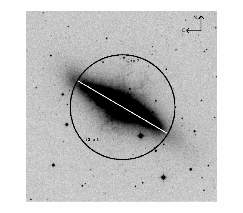
Figure 2.— Circular FOCAS field overlaid on DSS image centered on M 82. The white line approximately indicates the position of the narrow gap (5 arcsec) separating Chip 1 from Chip 2.

Figure 2 shows the observed field. The images can be divided into the following groups:

M 82 Images:
1. Off-band images of M 82.
2. On-band images of M 82.
3. On-band plus grism images of M 82.

Photometric Calibration Images:
1. On-band images of LTT 9491 (on each chip).

Slitless Spectroscopy Calibration Images:
1. On-band images of engineering mask illuminated by Th-Ar calibration lamp to acquire undispersed calibration positions.
2. On-band plus grism images of engineering mask illuminated by Th-Ar calibration lamp to acquire dispersed calibration spectra.

Slitless Spectroscopy Calibration Control Images:
1. On-band images of engineering mask illuminated by the large, local PN NGC 7293, to acquire undispersed source positions.
2. On-band plus grism images of engineering mask illuminated by NGC 7293 to acquire dispersed source spectra.
3. On-band plus grism images of engineering mask illuminated by Th-Ar calibration lamp to acquire dispersed calibration spectra.

Our data consist of six sets of observations (two on each night), where each set is comprised of one image from each of the three M 82 image types and the two slitless spectroscopy calibration image groups. In addition, nightly sets of photometric calibration images and slitless spectroscopy calibration control images. The use of these calibration control images will be fully described in § 5. All images underwent basic CCD reductions (bias subtraction and flat-field correction using sky flats) using IRAF standard tasks.

Table 1 lists the most important CCD images obtained for this project. Since there are two CCD images for each field (Chips 1 and 2), for brevity we have listed only the exposure number corresponding to Chip 1. For Chip 2, add 1 to the listed exposure number.

The six sets of on-band, off-band, and grism images were registered and combined for each of the two CCD chips. The IRAF procedure geomap was used to calculate appropriate registration shifts and imshift was used to perform these shifts. Registration errors for the on-band and off-band images were smaller than 0.2 pixels, however errors for the grism images were greater. Grism registration errors were typically 0.3 pixels, with one frame having an error of 0.5 pixels. Sets of registered images were combined and cosmic rays removed using imcombine and its cleaning algorithm minmax. The off-band combined image was then registered to the combined on-band image for PN identification purposes, while the combined grism image needed no registration to the combined on-band image, as it was imaged in an identical instrument position as the on-band.

When the observations were made, the field of view was oriented so that the major axis of M 82 would fall near the $5^{\prime\prime}$ gap between the two CCDs. This choice was made due to the expectation that very few PNe would be visible along the major axis of the galaxy because of heavy dust extinction and bright, confusing background continuum emission along the extent of the disk. For analysis and cataloging purposes, the major axis was defined by fitting to peaks in the galaxy continuum emission. Emission peaks were identified fitting a high-order polynomial to image cuts made in the minor axis direction through regions of smooth continuum emission located at the ends of the visible disk. Once the major axis was defined, we determined the minor axis to be the line perpendicular to the major axis that passed through the kinematic center of the galaxy. We adopted the kinematic center defined by Achtermann & Lacy (1995) at $\alpha$= $9^{\rm h}55^{\rm m}52^{\rm s}.14$ $\delta$=$69^{\circ}40^{{}^{\prime}}45^{\prime\prime}\!\!.90$, thus placing our major/minor axis coordinate center at $\alpha$= $9^{\rm h}55^{\rm m}51^{\rm s}.77$ $\delta$=$69^{\circ}40^{{}^{\prime}}50^{\prime\prime}\!\!.22$. These axes are rotated $4^{\circ}$ from the original pixel axes.

3.2. HST+ACS Observations

To complete our set of observations, we used a Hubble Space Telescope six-point mosaic H$\alpha$ image of the galaxy, observed using the ACS wide-field imager. These observations were made available via the Multimission Archive at STScI. For details on the observation and image reduction, please see Mutchler et al. (2007), but we include a short summary here. Twenty-four individual overlapping, dithered exposures from the ACS Wide Field Channel, consisting of two 2k$\times$4k pixel CCD chips, were combined to create a single 12k$\times$12k pixel (10.24$\times$10.24 arcmin) image. The image scale is $0^{\prime\prime}\!\!.05$ pixel^-1. Imaging was made through a F658N H$\alpha$ filter, with the following characteristics: effective central wavelength of 6584 Å, peak transmission of 44%, and FWHM width of 87 Å. The PSF FWHM is $\sim 0^{\prime\prime}\!\!.1$. The right-most panel of Figure 1 shows a cutout from the ACS H$\alpha$ image, to illustrate its excellent resolution in comparison to the FOCAS cutouts.

The mosaiced H$\alpha$ image has a total exposure time of 3320 s. When combined with a superior observing platform and space-based resolution, this image depth is more than adequately matched to our [Oiii] imaging. All candidate PN objects identified in the [Oiii] imaging were detected (S/N $>$ 3) in the H$\alpha$ image.

4. PN Identification

In § 2 we discussed using an on-band/off-band blinking technique for making PN identifications. The first step in applying this method was to produce additional images to aid our search. A version of each of the FOCAS combined images was created by using the IRAF fmedian filtering task to subtract the smooth background galaxy continuum emission. These resulting images proved to be essential in making PN identification within regions close to the major axis of the galaxy that before had bright, confusing backgrounds. In addition, an image was created using analysis software developed by Alard & Lupton (1998) and implemented in Munich by Gössl & Riffeser (2002) that carefully subtracts a properly scaled off-band image from an on-band image. The result is a high quality continuum subtracted image, where only desired emission line sources remain. This image not only aided in identification purposes, but will play an important role in our photometry work, as detailed in § 6.

We visually inspected our data using three initial selection criteria: detection in the on-band image, non-detection in the off-band image, and point source detection in the grism image. The result of this initial effort was the identification of 116 preliminary PN candidates. To obtain accurate coordinates for each of the candidates, we created a coordinate transformation from pixel coordinate positions on the FOCAS images to pixel coordinate positions on the ACS images using IRAF tasks geomap and geoxytran. Source identifications on the ACS images were confirmed by eye and accurate centers were calculated using imcentroid. Final coordinates were obtained using skyctran from the WCS coordinates embedded in the ACS image header. These WCS coordinates are good to 0.1 pixels, however the final accuracy of our positions are limited to $0^{\prime\prime}\!\!.05$ by the uncertainty of our centering results.

In our search for PNe in a late-type galaxy such as M 82, the risk of contamination from numerous supernova remnants (SNRs) and Hii regions in a galaxy with active on-going star formation is great. To combat this issue, we imposed two additional criteria for the confirmation of our PNe candidates: they appear as unresolved point sources with no visible extension and they show a characteristically high line ratio of $R=I([O\textsc{iii}])/I(H\alpha)$.

The criterion concerning the rejection of resolved sources or those showing visible extension is included to differentiate between true PNe and contaminants using a candidate’s angular size. Bright galactic PNe have sizes less than $\sim 1$ pc (Acker et al. 1992). At M 82’s distance of $\sim 3.5$ Mpc, this corresponds to an angular size for PNe of less than $0^{\prime\prime}\!\!.06$, which cannot be resolved in even our highest resolution H$\alpha$ image. Therefore, if we observe any resolved sources or extended structures in this image, these objects must have extents on the order of tens of parsecs, thus eliminating them as potential PNe. As further proof of this point, we conducted a search for known SNRs and Hii regions. Optical and radio surveys of these objects have mainly focused on the starbursting core, within 1 kpc of the nucleus (de Grijs, et al. 2000; Rodriguez-Rico et al. 2004). While this was not a favored region for PN discovery, due to the bright, confusing background, none of our PN candidates were coincident with these objects. Furthermore, these studies derived sizes of these objects that were all greater than $\sim 2$ pc, making them at least marginally resolved objects in our ACS imaging.

The final selection criterion for PN identification uses [Oiii] and H$\alpha$ data to calculate a line ratio between the two:

$$R=I([O\textsc{iii}])/I(H\alpha+[N\textsc{ii}]).$$ (1)

For simplicity, we will refer to the H$\alpha$ + [Nii] blend as simply H$\alpha$ emission throughout. While the previous criterion on resolved sources should eliminate most contaminants, there is still a possibility that compact Hii regions could still remain in our sample. An important distinguishing feature of PNe, however, is that the central stars responsible for the ionization of PNe are typically higher temperature objects than the stars that ionize Hii regions. Because of this fact, we expect the levels of doubly ionized oxygen emission, with respect to H$\alpha$ emission, to be higher in PNe than in Hii regions. A survey by Shaver et al. (1983) showed that most Hii regions $(\geq 80\%)$ have $R<1$. Therefore, we can assume that the line ratio, R, will in general be greater than one for PNe, while the opposite is true for Hii regions.

Herrmann et al. (2008) expand on this idea and use observations presented in Figure 2 of Ciardullo et al. (2002) to show the tendency of PNe to populate a distinctive region in [Oiii] - H$\alpha$ emission line space. Using this fact, they define a limiting R as a function of absolute [Oiii] magnitude in their Eqs. 2 & 3, below which PN candidates should be rejected. This boundary sets a stringent standard for the minimum allowable R value over the top $\sim 1.5$ mag of the PNLF, whose members are critical for making a PNLF distance determination. Figure 3 shows the positions of our M 82 sources in the Herrmann et al. (2008) plot. It should be noted that as this boundary is set relative to the absolute [Oiii] magnitude, distance is intrinsically incorporated into this plot. In addition, because we can assume that there will be some extinction from such a dusty, edge-on galaxy, we must also remind the reader that this plot is subject to extinction effects. These include extinction in [Oiii] that will tend to move objects to fainter absolute [Oiii] magnitudes and differential extinction that will lower R values.

Figure 3.— [Oiii]/H$\alpha$ ratio plotted as a function of the absolute magnitude $M$(5007), as defined in Section 5.1. The dashed diagonal line is the PNe-Hii boundary as defined by Herrmann et al. (2008) using the Dalcanton et al. (2009) TRGB distance to calculate $M$(5007). Sources located below the dashed diagonal line should be rejected as possible Hii regions, therefore the two candidates marked with asterisks were removed from the sample.

Of the 116 original candidates that satisfied the initial three criteria, we eliminated four due to suspicious extension and resolved sizes, one due to a low [Oiii]/H$\alpha$ ratio, and one that was disqualified by both of the additional criteria. Approximate derived sizes for the resolved objects ranged from $\sim 15-350$ pc. Even when allowing for up to $\sim 0.5$ mag of uncertainty in the x-axis location of objects in Figure 3, two objects clearly lie outside the accepted range of R values. One additional candidate was also removed due to an anomalous velocity measurement, which we will discuss more throughly in § 5. The seven rejected candidates, their positions, and other derived data can be found in Table 2. The remaining 109 objects that make up our final sample, their positions, and all other derived data, can be found in Table 3.

5. Radial Velocity: Calibration and Results

5.1. Calibration and Velocity Determination

We introduced the procedure to obtain slitless radial velocity measurements for our PN candidates in § 2. We will now describe the specific details behind the calibration procedure. The layout of points that sets up our calibration grid, for later use in bilinear interpolation, is created by placing an engineering mask, containing 970 holes in the desired 100 pixel interval grid pattern, into the light path. Illuminating the CCD with a Thorium-Argon calibration lamp through both the mask and the on-band filter defines the undispersed positions for each of the calibration points. After inserting the grism, the light from the calibration lamps is dispersed into the Th-Ar spectrum, from which the positions of five Th and Ar emission lines can be measured. The shifts from the undispersed to the dispersed positions for each of these known wavelengths are calculated, and the relation between shift and wavelength is determined, allowing for eventual wavelength interpolation for our PNe candidates. The accuracy of this calibration technique is explored in § 5.2.

Each candidate’s ($x$,$y$) pixel position on the median versions of the non-dispersed on-band image and the dispersed grism image were obtained using IRAF’s imcentroid task, and dispersion shifts were calculated for each source. After calibrating our data as described above, using a set of calibration images taken during the first night of observations, we used a custom bilinear interpolation code to calculate wavelengths and velocities for the PN candidates. Fifteen objects were left unmeasured due to their location on the image outside of the calibration grid, making complete, accurate interpolation impossible. In addition, one PN candidate was removed from the sample due to its extremely discrepant velocity of -251 km s^-1, as referred to in § 4. We assume this object is a background emission-line galaxy that has a redshifted emission line within the bandpass of the filter, thus explaining the single inconsistent measurement. After combining this single rejection with those already detailed in § 4, and considering those objects left unmeasured, we come to our final sample of 94 confirmed PNe with measured radial velocities. This velocity data, along with the previously mentioned positional data, are included in Table 3. The uncertainty in the velocities is 10 km s^-1, based upon the grism dispersion, seeing conditions, and uncertainty in image registration. The positions of these final velocity sample members, relative to the center of M 82, are shown in Figure 4. The $x$ and $z$ coordinates are defined, respectively, along the major and minor axis.

Figure 4.— Positions of the 94-member PN velocity sample, relative to the center of M 82. Coordinates $x$ and $z$ are measured along the major and minor axes, respectively. Dashed lines denote $z$ distance from the major axis of 55 arcsec, equivalent to $\sim 0.95$ kpc at the distance of M 82.

5.2. Calibration and Slitless Velocity Analysis

To confirm the accuracy of the slitless velocity measurements, we conducted two forms of analysis on our calibrations. The first analysis technique was simply to use a second set of calibration images to calibrate our velocities. The left panel of Figure 5 shows that the velocities determined using the different calibration files are virtually identical. The maximum difference between measurements was 3 km s^-1, and the mean difference was 1 km s^-1. The second portion of the analysis was to compare our technique of slitless velocity determination to that of a classical (slit) method. The local Galactic PN NGC 7293 was chosen as a test case. Images of NGC 7293 were taken in two different ways: an on-band image acquired through the engineering mask, with 970 holes covering the extent of the field of view, and a dispersed on-band image acquired through both the grism and the engineering mask. The angular size of NGC 7293 is such that it fills the entire field of view, so that by inserting the engineering mask, we create 970 point sources from our single target object. This provides us with an opportunity to measure velocities, at locations spread across the entire field of view, that should agree, on average, with the known velocity of NGC 7293. Some scatter is expected, due to variations in the PN’s expansion velocity field and density distribution that each contribute to dispersion in individual velocities measured at points across the field of view. We can make the radial velocity measurements in the same manner as for M 82, using our slitless method, or we can treat each hole as a slit and measure the velocity of the source in the classical way, by making a direct comparison of the dispersed location of the target emission line with the locations of the calibration spectral features. The right panel of Figure 5 shows that the velocities determined using the two different methods agree very well with each other. In addition, the average of 916 radial velocity measurements we obtained for NGC 7293 is $-32$ km s^-1, which shows close agreement with the known value of $-27$ km s^-1 (Meaburn et al. 2005). The scatter we find, from $-60$ to $-5$ km s^-1, is also in close agreement with the findings of other comparable observations of the NGC 7293 (see Fig. 8, Meaburn et al. 2005). From all these facts, we conclude that the uncertainty in our velocity measurements is at most 10 km s^-1.

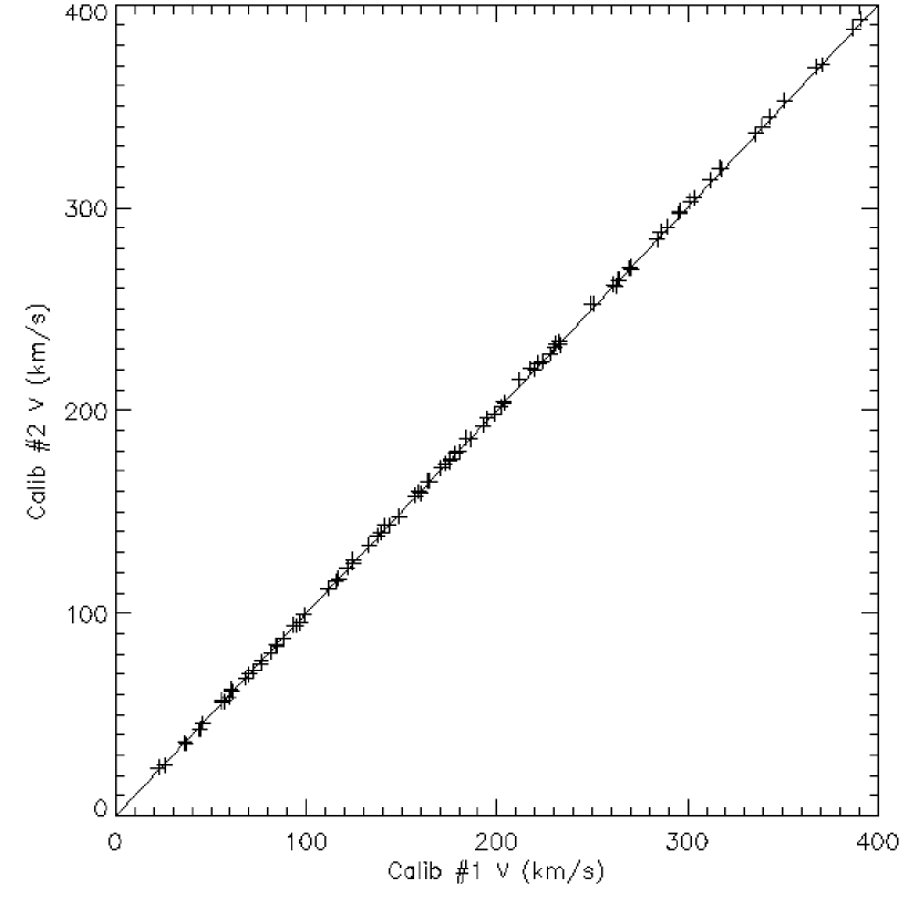
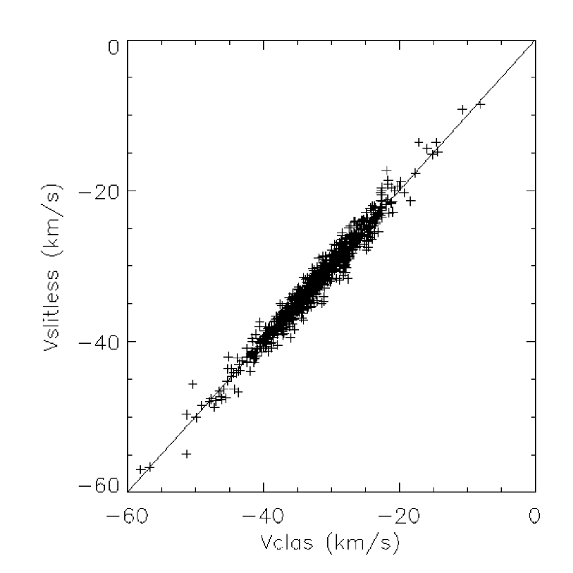
Figure 5.— Calibration analysis results. Left: Comparison of radial velocity measurements made for M 82 PN sample using two different sets of calibration images. Right: Comparison of radial velocity measurements made for NGC 7293 using classical and slitless techniques for velocity determination.

There is a final point to consider: the airmass of our NGC 7293 validation observations is smaller than that of our M 82 observations (see Table 1), and possible flexure in the FOCAS spectrograph might produce systematic velocity differences between these two telescope alignments. We can show that this is not the case by examining our previous study of PNe in NGC 4697 (Méndez et al. 2009). The observations of NGC 7293 used in that work were obtained at an airmass of about 1.8, which is similar to the airmass of our M 82 observations. Inspection of Section 4 and Figure 3 in Méndez et al. (2009) shows that there is no significant difference in the radial velocities measured across NGC 7293 with respect to what we find in our analysis, displayed in Figure 5. In other words, the mechanical stability of FOCAS is such that flexure effects are negligible for our purposes.

5.3. Velocity Results: Comparison With Existing Literature

Our velocity measurements of PNe in M 82 show the expected signature of a rotating disk. Figure 6 shows that the northeast, receding side of the disk (positive offset) is redshifted to velocities greater than that of the systemic velocity, while the southwest, approaching side of the disk (negative offset) is blueshifted to velocities less than that of the systemic velocity. This signature of the bulk rotation of the galaxy agrees with published M 82 velocity data (e.g. Sofue et al. 1992) and the trailing direction of its spiral arms (Mayya et al. 2005).

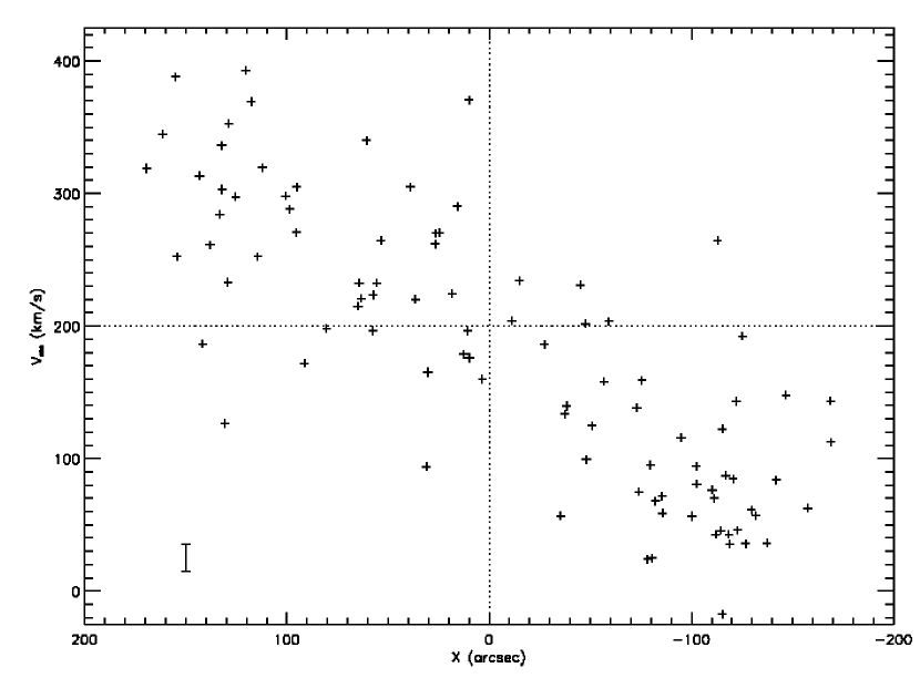
Figure 6.— Radial velocities of the complete velocity sample, numbering 94 PNe, plotted as a function of their major axis position. The error bar located in the bottom left is representative of the 10 km s^-1 uncertainty for each data point.

We also find agreement with values of M 82’s systemic velocity. Achtermann & Lacy (1995) and McKeith et al. (1993) both derived a systemic velocity for M 82 of 200 km s^-1 with uncertainties of 7 and 11 km s^-1 respectively. When we narrow our sample to 43 near-disk objects found within $\sim 0.5$ kpc ($29^{\prime\prime}\!\!$ ) of the major axis, to reduce the dilution of the rotational signature, we measure a systemic velocity of $195\pm 18$ km s^-1. This agreement with the literature value, within the range of uncertainty, provides further evidence of the accuracy of our data. In subsequent analysis for this study, we adopt the literature value of 200 km s^-1 for the systemic velocity, due to our measurement’s limited sample size.

Rotation curves are a standard tool central to the characterization of the kinematic properties of a galaxy. Sofue et al. (1992) presents a rotation curve for M 82, derived from CO(2-1) observations, that shows a peculiar, near-Keplerian decline, to which we would like to compare our results. Due to the uncertainty in the height from the galaxy mid-plane of our observed PNe, projecting the positions of these PNe onto the plane in order to plot a comparable rotation curve becomes problematic. Therefore, we choose instead to compare our results to a simulated observational signature we would expect from a PN population that follows the CO-derived rotation curve.

These simulations model the spatial and kinematic distributions of an observed PN population, which should help in the interpretation our velocity results. Spatially, we assume that PNe will be distributed radially in an exponential disk. For this exponential, we choose the K-band scale length, as derived by Mayya et al. (2005). For simplicity, we neglect adding a vertical scale height distribution and forgo modeling structural features such as spiral arms. To help fit our observations, we also include a second extincting exponential distribution, with a shorter scale length, which results in a final ring-like particle distribution that mimics the extinction towards the center of the galaxy that prevents any detections from this region. Particles are then randomly distributed according to this distribution and assigned velocities according to either a typical flat rotation curve or a falling rotation curve that matches the CO data. These velocities also take into account a velocity dispersion of 60 km s^-1, as is appropriate for a system with a peak rotational velocity of $\sim 200$ km s^-1 (Bottema 1993). The final step is to then take this simulated disk galaxy and transform its inclination and velocities to conform to our observed view, adopting an inclination of 77 degrees and a systemic velocity of 200 km s^-1 (Mayya et al. 2005; McKeith et al. 1993)

As we run each simulation, we bin the resulting velocity distributions into eight bins, according to their position along the observed major axis. By then binning our own data in the same manner, it is possible to see how our velocity distribution compares with that of our simulations. These binned results are plotted in Figure 7. This figure shows that we find good agreement between our binned velocities and the simulated falling rotation curve at positive $x$ positions. However, at negative $x$ positions, we find that our binned averages seem to fall directly between the simulated flat and falling rotation curve data points. One possible source of this discrepancy lies in our approximation of a featureless exponential disk. It appears that there is an overdensity of individual PN velocity data points in Figure 7 centered at approximately ($X$,$V$)=($-110$, 40). Interestingly, this grouping also appears in position space in Figure 4 at ($X$,$Z$)=($-110$, 25). One possibility for these groupings could be that these structures are part of the approaching, western spiral arm, as identified in Mayya et al. (2005). This would cause our observed velocities to differ from our idealized simulation due to a possible bias in the average binned velocity of our data.

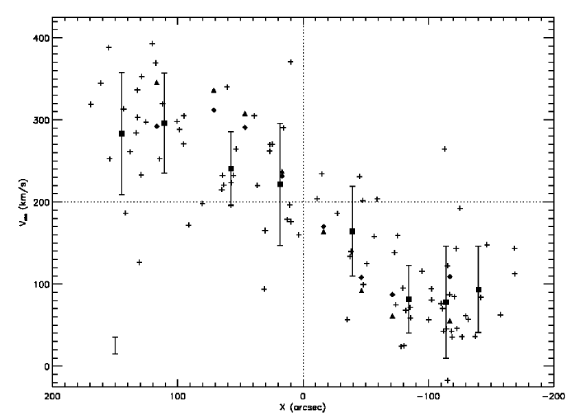
Figure 7.— Binned velocities of 94 PNe as a function of their major axis position. Our bins are represented by square symbols, where the numbers of PN in each bin, from left to right, are 11, 12, 11, 12, 12, 12, 12, 12. Bars on squares represent the dispersion within the binned velocities, in this case ranging from 41 to 75 km s^-1. Diamond symbols represent binned simulation results for a falling input rotation curve, while triangle symbols represent binned simulation results for a flat input rotation curve. Individual PN velocity data points, showing the radial velocity distribution of our sample, are denoted with plus signs. The error bar located in the bottom left is representative of the 10 km s^-1 uncertainty of each individual data point.

While it is possible, with a few caveats, to find agreement between our velocity data and simulations of a declining, near-Keplerian rotation curve, we cannot be completely sure with regard to the shape of the rotation curve of our PN population. However, the multiple pieces of evidence presented in this section certainly favor agreement between the kinematic picture depicted by our PN velocities and published data found in the literature.

5.4. Velocity Results: PNe at High $z$

It is immediately apparent in Figure 4 that we have identified many PNe at rather large values of $z$. Given the inclination of approximately 77 degrees (Mayya et al. 2005), this indicates that these objects are likely to lie at large heights above the galactic plane. Assuming a distance to M 82 of 3.55 Mpc, PNe at $z>55$ arcsec are located $\sim 0.95$ kpc from the plane when projected from the major axis.

Figure 8 shows a comparison of the rotation shown by two PN groups in M 82: those PNe with $z<30$ arcsec are displayed in the left plot, while those with $z>55$ arcsec are displayed in the right plot. The substantial rotation at high $z$, comparable to the rotation found near the major axis, is remarkable. This result conflicts with the findings of Sofue et al. (1992) who, using CO velocities, found slow rotation speeds in the range of 20-30 km s^-1 at $z\sim 1$ kpc, and little or no rotation at $z>1.4$ kpc.

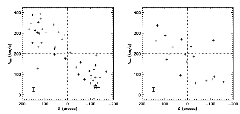
Figure 8.— Left: PN radial velocity as a function of $x$ coordinate, for PNe with $z<30$ arcsec. Right: Same, for PNe with $z>55$ arcsec. The systemic velocity of M 82 is 200 km s^-1, and the error bar located in the bottom left of each plot is representative of the 10 km s^-1 uncertainty for each data point.

The presence of bright PNe at high $z$ is certainly not unique to M 82. For example, Ciardullo et al. (1991) found 33 PNe in the edge-on galaxy NGC 891, 21 of which were more than 1 kpc distant from the galactic plane. These authors attributed the high-$z$ PNe to a spheroidal component of NGC 891, presumably an old population, and used this as an argument favoring the universality of the PNLF and its usefulness as a distance estimator. Are the high-$z$ PNe in M 82 also representatives of a stellar halo? Figure 9 shows a histogram with the number of PNe as a function of $z$, with 20 arcsec bins. The distribution is roughly fitted if we assume an exponential function with a scale height of 500 pc. A similar exercise involving the 33 PNe in NGC 891 gives more or less the same result.

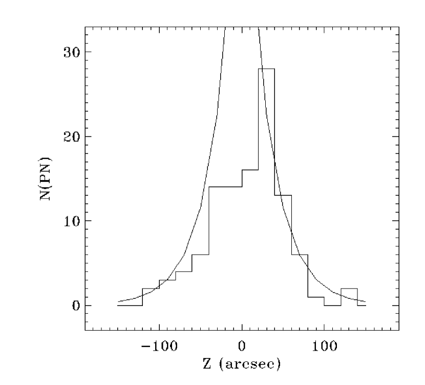
Figure 9.— Histogram showing number of PNe as a function of $z$ coordinate, with 20 arcsec bins. The distribution is fitted with an exponential function having a scale height of 30 arcsec, equivalent to $\sim 500$ pc at the distance of M 82.

A rotating halo population is not the only possible interpretation. As mentioned in § 1, there is strong evidence for a recent tidal interaction between M 81 and M 82. While none of our PNe lie coincident with any of these documented tidal features (Yun et al. 1994), nor do they show any outstanding peculiar motions, it can be argued that the disk of M 82 is very thick because it has been dynamically heated by the past interaction with M 81; so the high-$z$ PNe could be attributed to a disturbed, thick disk component.

Also, one could argue that because M 82 has been found to have an extended disk, reaching out to $\sim 12$ kpc (Davidge 2008), these objects may in fact be members of the outer disk, found close to the galaxy midplane, seen in projection. For instance, a $z$ distance of 55 arcsec translates to a position on the galaxy mid-plane $\sim 4$ kpc from the center, if it is projected straight towards the observer. In this situation, however, the conflict increases between the Sofue et al. (1992) rotation curve and our observed PN velocities, as objects rotating on the edge nearest to the observer should have the smallest radial velocities, due to their high tangential velocity component. Furthermore, PNe at these great radii should have extremely small rotational speeds according to a falling rotation curve, thus making this explanation of the high-$z$ rotation less attractive.

Of these three possibilities for the origin of the high rotational velocities sustained by these high-$z$ objects, our current data is insufficient to provide any further elucidating interpretation. One way to investigate this question further would be to obtain abundance measurements of these high-$z$ objects; a preponderance of low metallicities would confirm the stellar halo interpretation, and high metallicities would favor an extreme thick disk. Without such information, we cannot accurately make any further interpretation of our results and leave this as an open question for subsequent research.

6. Photometry, PNLF, and Distance

6.1. [OIII] $\lambda$5007 Photometry

In order to build our observed PNLF and obtain a distance estimate for M 82, we must first obtain [Oiii] $\lambda$5007 magnitudes for each of our PN candidates. These magnitudes are expressed using the standard definition for magnitudes $m(5007)$ from Jacoby (1989),

$$m(5007)=-2.5\;log\;I(5007)-13.74.$$ (2)

We conducted photometry on our imaging data, analyzing each of the FOCAS CCD chips separately, due to slight photometric differences that exist between the two chips. Our measurements were calibrated using observations of our spectrophotometric standard star, LTT 9491 (Colina & Bohlin 1994). Large aperture photometry using the IRAF phot task was conducted on single reference frames for our standard star and three bright, isolated, internal standard stars in our target field. This tied the spectrophotometric standard to our images, and we continue from this point forward using differential photometry.

These internal frame standards were then measured using a small aperture on the combined on-band frame, which allowed us to calculate an aperture correction, as well as a correction that accounted for non-photometric conditions introduced in the image stacking process. From here, we switch to PSF-fitting photometry using the DAOPHOT package (Stetson 1987) and its psf and allstar tasks. Using the internal frame standards, and four bright PN candidates as additional standards, we measure PSF aperture corrections and then perform PSF-fitting photometry on both the continuum subtracted image and the box median subtracted image for all 109 PN candidates.

Two further photometric corrections were also performed. The first accounted for a difference in airmass between the standard star image $(X=1.28)$ and our reference image $(X=1.77)$ that affected the photometry at the point when we tied our spectrophotometric standard to our internal frame standards. This represents only a small $-0.06$ mag correction to our measured, apparent magnitudes. The second correction accounted for filter transmission so that total physical fluxes from the emission lines could be properly measured. Following a procedure set out in Jacoby, Quigley, & Africano (1987), we make our correction based on the filter transmission of the redshifted wavelength of the [Oiii] $\lambda$5007 line, which is 5010 Å  considering M 82’s systemic velocity of 200 km s^-1. Transmission at this wavelength is at the filter’s peak value of 68%, and the corresponding magnitude correction for this transmission is $-0.419$ mag.

We then derived Jacoby magnitudes for all of our PN candidates. Magnitudes were measured on both continuum subtracted and median images, and preference was given to magnitudes derived from the continuum subtracted images whenever these measurements were possible. Magnitudes derived from the median image were used when sources lay on unusable portions of the continuum subtracted image (masked regions that contained bad pixels, saturated stars, regions of bright background galaxy emission). In all, 105 of 109 sources were successfully measured, and their $m(5007)$ magnitudes are listed in the source catalog found in Table 3.

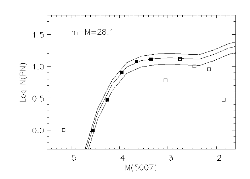
Figure 10.— Observed [O iii] $\lambda$5007 PNLF with 84 PNe binned at 0.3 mag intervals. Fits are made to the filled squares, while the open squares on the right denote bins beyond our incompleteness threshold, and the open square on the left denotes the bin for our single outlier object, PN 104. The absolute magnitudes are calculated using a best fit distance modulus of $m-M=28.1$ and a foreground extinction correction of 0.28 mag. The fitted theoretical PNLF is shown with sample sizes of 810, 690, and 550 PNe (see Méndez and Soffner 1997).

6.2. PNLF Construction and Fitting

From the sources with measured Jacoby magnitudes, we would like to select a statistically complete sample of PNe from which to build an accurate PNLF. Objects chosen for this sample come from regions in the field of view where we are confident in our measurement of a complete population. We want to eliminate PNe detected in regions of high galaxy background emission where PNe above our photometric incompleteness limit would still miss being detected because of their inability to rise above high background flux levels. In order to accomplish this, we lay down an isophote at the boundary where obvious, bright continuum emission becomes an obstacle to our PN identifications, and eliminate objects from the statistical sample that fall within this region. Also, we make a visual inspection of both our on-band and high-resolution H$\alpha$ images in order to reject objects that lie on or near obvious dust features. While defining these criteria remains a subjective practice, the total number of objects that contribute to our PNLF make our final result quite invariant to slight changes in this selection process.

In the end, we select 84 PNe for our statistical sample. From these selected [Oiii] $\lambda$5007 magnitudes, we build our PNLF. To this distribution, we fit a theoretical PNLF curve generated as in Méndez & Soffner (1997). We could have used more recent PNLF generation procedures, like in Méndez et al. (2008), but the end result at the bright end of the PNLF, which is what we use in PNLF distance determinations, is indistinguishable. The simulated PNLF is fit to our distribution and plotted in Figure 10.

There are many sources of uncertainty to consider when determining the final factor of error for our distance determination. Photometric error and uncertainty in the PNLF fitting process each account for sources of random error, at 0.1 mag each. We also include 0.05 mag of uncertainty for filter calibration into this factor of random error. However, we must also consider systematic errors, such as uncertainty in the distance to M 31, the calibrating galaxy for the PNLF distance measurement. Following Jacoby et al. (1990), these account for 0.13 mag of error in total. When added quadratically, random and systematic sources total to our final error estimate of 0.2 mag.

By combining our best fit PNLF with an adopted galactic extinction of $A_{5007}=0.28$ mag (see discussion below), our derived distance modulus is $28.1\pm 0.2$, which is equivalent to a distance of $4.2\pm 0.4$ Mpc.

6.3. Galactic Foreground and Internal Extinction Effects

One critical component of our distance determination lies in our adopted value of galactic foreground extinction. While Schlegel et al. (1998) has become a standard source for extinction values, we argue here that their value of $A_{V}=0.526$ is incorrect. Upon examining the dust maps from which the Schlegel et al. values are derived, it becomes immediately apparent that M 82’s emission contribution was left unsubtracted from this galactic map and our target is therefore assigned an inappropriately high extinction value. Figure 11 shows contours created from the dust map overlaid atop an optical DSS image of the nearby field of view, which includes the nearby galaxy M 81. This figure clearly shows the point source nature of this emission.

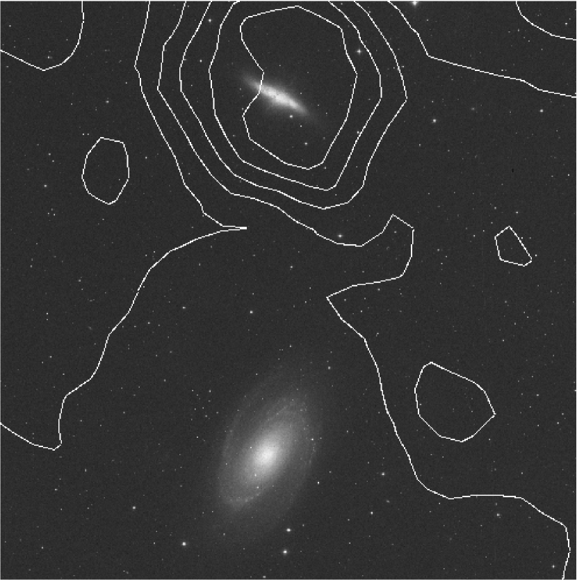
Figure 11.— Schlegel et al. (1998) dust map contours overlaid on DSS image of M 81/M 82 sky field. Image is in standard orientation with north up, east left.

Under further scrutiny, the situation actually worsens. The region of sky surrounding M 81 and M 82 has long been known to host troublesome highly spatially-variable foreground galactic extinction. Sandage (1976) presents an image of bright, filamentary reflection nebulae covering the entire field around these two galaxies. With such highly variable nearby structure, the reader should note that any single value of foreground extinction is simply an estimation which carries a considerable amount of uncertainty. To carry out a robust foreground extinction correction, individual estimates towards each PN should be made. However, as the uncertainty of internal extinction dominates over the foreground component, we will continue to use a simple single-value approximation here.

In an effort to choose a proper foreground extinction estimation, we exclude the value given by Burstein & Heiles (1984) of $A_{V}=0.09$ as unreasonably low. We instead adopt a value of $A_{V}=0.25$ from Dalcanton et al. (2009), who interpolated the value of extinction at M 82’s position from nearby, non-contaminated values in the Schlegel et al. (1998) dust map. For comparison, M 81 has a listed value of $A_{V}=0.26$. Assuming a standard R=3.1 dust curve, this translates to our adopted foreground extinction value of $A_{5007}=0.28$.

Our derived distance measurement of 4.2 $\pm 0.4$ Mpc is quite discrepant from the Dalcanton et al. (2009) TRGB-derived value for M 82 of 3.55 $\pm 0.06$ Mpc . We note that Sakai & Madore (1999) also make a TRGB distance determination to M 82, however the Dalcanton et al. (2009) value takes precedence due to their superior data quality, star counts, and observational footprint away from obscuring dust. In addition, we also derive a larger distance than those derived for group member M 81: 3.63 $\pm 0.34$ Mpc as calculated by Freedman et al. (1994) using Cepheid variables, and 3.50 $\pm 0.40$ as calculated by Jacoby et al. (1989) using a similar PNLF fitting technique. In order to reconcile this distance discrepancy, we point to internal extinction within M 82 as the most likely culprit. As stated in § 1, M 82 is a starbursting system with ongoing star formation; it should be assumed to contain large amounts of obscuring dust throughout the plane of the galaxy, into which we look edge-on. As evidence of this fact, Puxley (1991) estimates extinction as high as $A_{V}=27$ to the center of the galaxy. Engelbracht et al. (2006) studied a Spitzer IRAC image at 8$\mu$m where they showed that emission from hot dust was not only distributed throughout the plane, but also at heights up to 6 kpc from the plane. Not only is the amount of dust plentiful in this system, but also distributed over a large extent, both in the plane and vertically. To compare the positional distribution of our objects to the dust distribution surrounding M 82, we overlay the positions of our objects on this same 8$\mu$m image in Figure 12.

One method to investigate how internal extinction is affecting our PNLF is to study two sub-samples of the PNe: objects at greatest risk to internal extinction and those least susceptible to such effects. In most cases, these sub-samples would show systematically different photometric results, and this would help to constrain the effect of internal extinction on our results. To attempt this exercise, we first divide our sample according to minor axis offset, considering that PNe that lie towards the plane have a greater likelihood of suffering from internal extinction from dust that lies predominately in the plane. Next, we assign our sub-samples according to the amount of 8$\mu$m dust emission detected at the positions of our PN objects, which takes into consideration the dust that is known to lie vertically away from the plane. Unfortunately, no detectable systematic differences in the magnitude distributions were observed for sub-samples defined by either method. The failure of this exercise may stem from the fact that projection effects may cause a considerable variation of internal extinction across small projected spatial scales, thus foiling any systematic search for such a correlation.

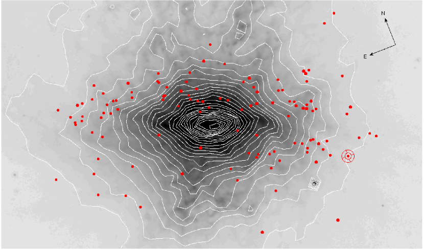
Figure 12.— Positions of the full 109-member PN sample overlaid on a SINGS IRAC 8 $\mu$m image (Kennicutt 2003) showing hot dust emission in M 82. The location of outlier PN 104 is denoted by the target symbol.

One observational signature that indeed suggests that internal extinction is responsible for our distance discrepancy appears as a lone outlier in our PNLF. This single PN, ID = 104, appears $\sim 0.5$ magnitudes brighter than the rest of the distribution. While other PNLF studies suggest that these outliers might merely be persistent contaminants, it is important to note that this PN candidate was throughly analyzed and cleanly passes all five selection criteria. We postulate that this object, unlike the majority of the rest of our sample, does not suffer from any great amount of internal extinction. To support this claim, we point out that in Figure 12, this single object appears offset from the galaxy center by $\sim 170$ arcsec in a region with little apparent dust in any of our images. There are only four other PNe who appear at locations with less 8$\mu$m emission, thus suggesting that this notion of an exception to our otherwise extreme internal extinction is not unfounded. Also, it is interesting to note that if this were indeed the single brightest PN in M 82 and we were to fit our PNLF with a sensible sample size to this single data point, we would derive a $\sim 0.4$ mag lower best-fit distance modulus. This new distance modulus of $27.7\pm 0.2$ would agree well with the Dalcanton et al. (2009) distance modulus of $27.75\pm 0.04$, along with many of the other comparable distance measurements. In particular, when assuming the same foreground dust extinction estimate as used above, we can overlay the position of PN 104 to fit perfectly along the best-fit PNLF derived by Jacoby et al. (1989) for M 81, as plotted in Figure 13.

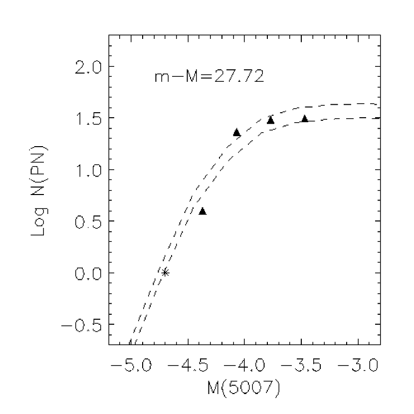
Figure 13.— Triangle symbols represent observed [O iii] $\lambda$5007 PNLF for 88 PNe in M 81 from Jacoby et al. (1989) plotted with our simulated PNLF function to their best-fit distance modulus of $m-M=27.72$ and a foreground extinction correction of 0.36 mag. The theoretical curves are shown for sample sizes of 2200 and 1600 PNe (see Méndez and Soffner 1997). The asterisk symbol denotes the location of our outlier PN 104 when considered at the same distance modulus and a foreground extinction correction of 0.28 mag.

While the pieces fall into place well for the case that our data suffers from a few tenths of a magnitude of internal extinction, the only true way to answer how much internal extinction affects our PNLF would be to acquire spectra for each of our PNe and measure individual extinctions to each object by means of the Balmer decrement. With these observations, we would be able to correct for extinction on a point-by-point basis, instead of using broad statistical corrections at a cost of increased uncertainties.

7. Summary of Conclusions

Using a method of slitless spectroscopy, we have detected 109 PNe in M 82, measured their radial velocities, and performed their photometry. We have carefully calibrated the radial velocity procedure and we have tested it using observations of the local Galactic PN NGC 7293. We find radial velocity uncertainties to be below 10 km s^-1.

The average radial velocity of PNe close to the major axis in M 82 shows excellent agreement with previous velocity studies of the galaxy obtained by other methods (i.e. CO emission), further confirming our error estimates. The individual radial velocities of PNe in M 82 show a clear rotational signature, again in excellent agreement with previous studies. Through simulations, we find that our data also agrees with a near-Keplerian rotation curve, though this conclusion is not definitive. Also, we discover that PNe who appear at high $z$ positions also show a clear rotational signature, which conflicts with an earlier published result that claims there is little or no rotation away from the disk. Additional observations are required in order to pin down whether these peculiar objects are part of a halo population or members of a thick disk population.

Our derived PNLF shows several indications that our PN photometry suffers from considerable internal extinction, on the order of 0.3 or 0.4 mag, thus explaining our discrepant distance modulus of $28.1\pm 0.2$ and its associated distance of 4.2 $\pm 0.4$ Mpc. Additional spectroscopy of these PNe would allow us to derive individual extinction measurements and improve upon our current measurement.

Table 1FOCAS observations and calibrations

FOCAS Field	Configuration	FOCAS number	Exp (s)	Airmass
M 82	Off-band	55749	60	1.88
M 82	On-band	55751	600	1.87
M 82	On+grism	55753	1000	1.82
Th-Ar + mask	On+grism	55757	10	1.76
Th-Ar + mask	On-band	55759	4	1.75
M 82	Off-band	55761	30	1.73
M 82	On-band	55763	300	1.73
M 82	On+grism	55765	500	1.71
NGC 7293 + mask	On-band	55855	200	1.36
NGC 7293 + mask	On+grism	55857	300	1.35
Th-Ar + mask	On+grism	55859	4	1.34
NGC 7293 + mask	On-band	55869	200	1.32
NGC 7293 + mask	On+grism	55871	300	1.32
Th-Ar + mask	On+grism	55875	4	1.32
LTT 9491	On-band	55877	10	1.28
LTT 9491	On-band	55879	20	1.28
LTT 9491	On-band	55881	10	1.28
LTT 9491	On-band	55883	20	1.28
M 82	Off-band	55963	60	1.78
M 82	On-band	55965	600	1.77
M 82	On+grism	55967	1000	1.73
M 82	Off-band	55975	60	1.67
M 82	On-band	55977	600	1.66
M 82	On+grism	55979	1000	1.64
NGC 7293 + mask	On-band	56035	200	1.35
NGC 7293 + mask	On+grism	56037	300	1.34
Th-Ar + mask	On+grism	56041	4	1.33
LTT 9491	On-band	56053	10	1.29
LTT 9491	On-band	56055	20	1.29
LTT 9491	On-band	56057	10	1.28
LTT 9491	On-band	56059	20	1.28
M 82	Off-band	56143	60	1.78
M 82	On-band	56145	600	1.77
M 82	On+grism	56147	1000	1.74
Th-Ar + mask	On+grism	56151	10	1.69
Th-Ar + mask	On-band	56155	4	1.68
M 82	Off-band	56157	60	1.67
M 82	On-band	56159	600	1.67
M 82	On+grism	56161	1000	1.64

Table 2Rejected PN Candidates

ID	X	Z	$\alpha$			$\delta$			Helio. RV
Number	(arcsec)	(arcsec)	(J2000)			(J2000)			(km s-1)	m(5007)	Rejection
224	-55.065	37.755	09	55	39.374	69	41	02.12	165.16	26.691	Extension
227	-55.007	23.652	09	55	40.472	69	40	49.34	173.72	25.062	H$\alpha$
124	-57.562	-41.564	09	55	45.124	69	39	50.01	227.81	26.524	Extension
233	-20.144	26.379	09	55	46.317	69	41	05.96	117.06	25.252	Extension
126	-33.043	-10.824	09	55	46.966	69	40	27.94	174.89	23.043	Ext. & H$\alpha$
127	-67.446	-132.141	09	55	50.400	69	38	24.36	-251.38	25.864	Velocity
236	2.311	16.472	09	55	51.034	69	41	06.18	179.60	24.809	Extension

Note. — The X and Z coordinates have their origin at $\alpha$= $9^{\rm h}55^{\rm m}51^{\rm s}.77$ $\delta$=$69^{\circ}40^{{}^{\prime}}50^{\prime\prime}\!\!.22$, where X and Z are defined along the major and minor axes, respectively.

Table 3Detected PN Candidates

ID	X	Z	$\alpha$			$\delta$			Helio. RV
Number	(arcsec)	(arcsec)	(J2000)			(J2000)			(km s-1)	m(5007)	Notes
201	-145.526	136.956	09	55	16.227	69	41	54.71	$\mathellipsis$	27.006	S
101	-202.709	-11.699	09	55	17.880	69	39	19.30	$\mathellipsis$	24.744	S
102	-194.546	-8.568	09	55	18.996	69	39	25.25	$\mathellipsis$	24.878	S
202	-133.872	124.036	09	55	19.192	69	41	47.88	$\mathellipsis$	25.526	S
203	-157.579	61.217	09	55	19.918	69	40	41.65	62.54	26.836	S
204	-168.920	24.166	09	55	20.843	69	40	03.77	112.33	25.795	S
103	-181.553	-14.324	09	55	21.642	69	39	25.15	$\mathellipsis$	25.655	S
205	-165.199	15.045	09	55	22.155	69	39	57.03	$\mathellipsis$	24.272	S
275	-165.166	14.491	09	55	22.217	69	39	56.52	$\mathellipsis$	25.131	S
104	-168.716	-36.910	09	55	25.566	69	39	09.89	143.52	23.301	S
206	-116.901	66.628	09	55	26.435	69	41	03.15	87.36	25.560	S
207	-112.919	62.136	09	55	27.482	69	41	00.67	264.42	26.442	S
208	-110.247	65.230	09	55	27.684	69	41	04.49	76.40	26.173	S
209	-114.516	52.567	09	55	27.929	69	40	51.40	45.76	24.711	S
210	-126.841	20.083	09	55	28.326	69	40	16.97	35.61	25.482	S
211	-120.499	29.271	09	55	28.694	69	40	27.92	84.49	24.933	S
105	-141.819	-19.293	09	55	28.789	69	39	36.46	83.94	25.606	S
212	-122.718	17.244	09	55	29.239	69	40	16.10	46.05	25.166	S
106	-146.651	-36.563	09	55	29.304	69	39	18.94	147.85	24.602	S
213	-115.346	24.809	09	55	29.940	69	40	25.88	122.30	24.789	S
214	-115.254	19.696	09	55	30.338	69	40	21.33	-17.54	25.417	S
107	-137.401	-29.834	09	55	30.354	69	39	28.68	36.14	25.785	S
108	-131.814	-23.061	09	55	30.776	69	39	37.02	56.92	26.233
215	-111.224	20.299	09	55	30.994	69	40	23.46	69.99	25.729	S
109	-125.155	-18.145	09	55	31.556	69	39	44.12	192.32	25.514
110	-122.160	-18.962	09	55	32.142	69	39	44.61	143.14	25.850
216	-102.429	22.912	09	55	32.302	69	40	29.42	94.00	24.485	S
217	-100.137	27.390	09	55	32.361	69	40	34.45	56.40	23.749	S
111	-129.677	-45.397	09	55	32.904	69	39	17.71	61.16	24.885	S
218	-94.876	27.588	09	55	33.249	69	40	36.76	115.83	25.612	S
112	-159.255	-115.145	09	55	33.304	69	38	03.50	$\mathellipsis$	25.909	S
113	-118.861	-28.890	09	55	33.462	69	39	36.85	35.52	24.330	S
219	-85.699	41.002	09	55	33.806	69	40	52.67	58.71	26.105	S
220	-79.817	53.573	09	55	33.857	69	41	06.43	95.05	25.136	S
114	-118.427	-33.846	09	55	33.928	69	39	32.58	42.83	25.230	S
115	-111.888	-23.672	09	55	34.278	69	39	44.45	42.71	26.143	S
221	-80.695	40.060	09	55	34.728	69	40	53.80	24.91	25.039	S
222	-93.733	9.993	09	55	34.801	69	40	21.30	$\mathellipsis$	$\mathellipsis$
116	-102.588	-23.283	09	55	35.832	69	39	48.54	80.61	24.618	S
223	-74.015	25.360	09	55	37.031	69	40	43.11	74.90	24.727	S
225	-50.682	43.496	09	55	39.692	69	41	09.22	124.81	24.751	S
226	-44.966	53.954	09	55	39.885	69	41	20.92	231.09	26.354	S
117	-85.562	-44.888	09	55	40.481	69	39	35.78	71.57	25.802	S
118	-78.220	-34.265	09	55	40.930	69	39	48.32	24.03	26.249	S
228	-38.376	48.845	09	55	41.424	69	41	19.00	139.57	24.485	S
229	-48.021	20.959	09	55	41.904	69	40	49.65	99.32	25.967
119	-72.892	-37.564	09	55	42.108	69	39	47.51	138.35	25.889	S
120	-75.375	-54.511	09	55	43.004	69	39	31.18	159.16	26.207	S
121	-56.824	-15.421	09	55	43.187	69	40	14.24	157.94	25.845
230	-14.902	69.494	09	55	43.873	69	41	47.32	234.07	26.115	S
122	-82.030	-81.482	09	55	43.952	69	39	04.10	67.92	24.960	S
231	-37.324	15.586	09	55	44.191	69	40	49.17	133.61	24.181
123	-59.248	-38.159	09	55	44.533	69	39	52.54	203.52	27.042	S
232	3.495	92.526	09	55	45.331	69	42	15.56	159.98	26.462	S
125	-47.574	-37.199	09	55	46.491	69	39	58.03	201.88	25.009	S
234	-11.200	28.132	09	55	47.770	69	41	11.37	203.90	25.508
235	10.607	72.570	09	55	48.120	69	42	00.43	196.41	25.265	S
128	-35.211	-70.671	09	55	51.228	69	39	32.76	56.54	25.927	S
129	-27.275	-57.126	09	55	51.579	69	39	48.17	185.94	26.948	S
237	9.864	23.792	09	55	51.782	69	41	15.83	176.03	25.370
238	26.476	57.809	09	55	52.048	69	41	53.50	269.85	26.180	S
239	18.273	38.672	09	55	52.084	69	41	32.79	224.30	26.630	S
240	15.678	23.991	09	55	52.788	69	41	18.47	290.38	25.684
241	12.693	11.284	09	55	53.259	69	41	05.66	178.72	25.234
242	30.448	46.753	09	55	53.618	69	41	45.15	165.07	26.027	S
243	24.555	25.568	09	55	54.211	69	41	23.44	270.29	25.981
244	26.764	30.331	09	55	54.229	69	41	28.69	261.99	26.008	S
245	36.476	35.505	09	55	55.522	69	41	37.25	220.12	25.560	S
130	10.011	-32.892	09	55	56.201	69	40	25.37	370.60	25.739
246	39.033	17.096	09	55	57.387	69	41	21.45	304.91	25.346
247	53.594	39.257	09	55	58.219	69	41	47.56	264.42	$\mathellipsis$
248	64.343	55.899	09	55	58.802	69	42	06.97	232.40	$\mathellipsis$
249	55.625	29.140	09	55	59.356	69	41	39.26	232.55	25.054
250	63.310	44.899	09	55	59.479	69	41	56.64	220.82	24.849	S
251	64.794	46.037	09	55	59.655	69	41	58.28	215.06	25.634	S
252	57.287	28.390	09	55	59.714	69	41	39.22	223.46	24.867
253	57.531	24.198	09	56	00.075	69	41	35.50	196.44	25.851
131	31.081	-64.879	09	56	02.358	69	40	04.81	93.79	26.178	S
132	60.722	-19.241	09	56	04.005	69	40	58.36	340.08	23.840
254	95.367	31.718	09	56	06.073	69	41	57.57	270.73	24.670	S
255	100.668	42.853	09	56	06.133	69	42	09.73	298.15	24.260	S
256	95.192	25.388	09	56	06.527	69	41	51.71	305.05	25.034	S
257	114.435	21.569	09	56	10.153	69	41	55.94	252.49	25.112	S
258	112.151	11.089	09	56	10.539	69	41	45.48	319.64	24.436
259	117.595	20.688	09	56	10.793	69	41	56.46	369.32	24.794	S
133	91.250	-58.375	09	56	12.299	69	40	35.07	171.79	25.404	S
260	130.628	29.174	09	56	12.359	69	42	09.24	126.48	25.025	S
261	120.283	5.840	09	56	12.404	69	41	43.97	392.85	25.563
262	125.468	15.685	09	56	12.530	69	41	54.99	297.28	24.508	S
263	141.626	38.460	09	56	13.553	69	42	22.06	186.35	25.309	S
264	128.699	5.624	09	56	13.884	69	41	47.25	352.74	24.389
134	80.541	-107.137	09	56	14.172	69	39	46.60	198.22	24.896	S
265	132.073	-0.017	09	56	14.877	69	41	43.32	302.95	25.073
266	143.288	21.424	09	56	15.162	69	42	07.28	313.53	25.594	S
135	129.293	-24.114	09	56	16.221	69	41	21.41	232.96	24.350	S
136	98.689	-94.201	09	56	16.312	69	40	05.75	288.07	25.912	S
267	155.104	16.468	09	56	17.592	69	42	07.52	388.14	26.875	S
137	141.628	-19.384	09	56	17.999	69	41	30.70	$\mathellipsis$	24.072	S
268	154.513	0.252	09	56	18.688	69	41	52.55	252.46	24.299	S
269	161.506	14.006	09	56	18.839	69	42	07.80	344.87	25.516	S
138	133.244	-51.032	09	56	18.969	69	40	58.71	284.32	24.820	S
270	155.134	-4.830	09	56	19.193	69	41	48.22	$\mathellipsis$	24.416	S
271	163.421	-7.060	09	56	20.801	69	41	49.57	$\mathellipsis$	25.245	S
272	162.508	-9.450	09	56	20.827	69	41	46.92	$\mathellipsis$	$\mathellipsis$
139	138.071	-69.051	09	56	21.182	69	40	44.21	261.26	25.842	S
273	169.387	-0.872	09	56	21.341	69	41	57.47	319.03	24.382	S
140	132.240	-94.696	09	56	22.111	69	40	18.79	336.34	25.776	S
274	185.345	7.267	09	56	23.405	69	42	10.99	$\mathellipsis$	24.954	S
141	184.188	-78.470	09	56	29.704	69	40	54.19	$\mathellipsis$	25.645	S

Note. — The X and Z coordinates have their origin at $\alpha$= $9^{\rm h}55^{\rm m}51^{\rm s}.77$ $\delta$=$69^{\circ}40^{{}^{\prime}}50^{\prime\prime}\!\!.22$, where X and Z are defined along the major and minor axes, respectively. An “S” denotes membership in the statistical sample used for PNLF fitting.

References

- (1) Achtermann, J.M., & Lacy, J.H. 1995, ApJ, 439, 163
- (2) Acker, A. et al. 1992, Strasbourg-ESO Catalogue of Galactic Planetary Nebulae (Garching:ESO)
- (3) Alard, C., & Lupton, R.H. 1998, ApJ, 503, 325
- (4) Arnaboldi, M., et al. 2008, ApJ, 674, L17
- (5) Bottema, R. 1993,A&A, 275,16
- (6) Burstein, D., & Heiles, C. 1984, ApJS, 54, 33
- (7) Ciardullo, R., et al. 2002, ApJ, 577, 31
- (8) Ciardullo, R. 2003, in IAU Symp. 209, Planetary Nebulae: Their Evolution and Role in the Universe, ed. S. Kwok, M. Dopita & R. Sutherland (San Francisco: ASP), 617
- (9) Ciardullo, R., et al. 1991, ApJ, 383, 487
- (10) Colina, L., & Bohlin, R.C. 1994, AJ, 108, 1931
- (11) Cottrell, G. A. 1977, MNRAS, 178, 577
- (12) de Grijs, R., et al. 2000, AJ, 119, 681
- (13) Dalcanton, J., et al. 2009, ApJS, submitted
- (14) Davidge, T.J. 2008, AJ, 136, 2502
- (15) De Lorenzi, F., et al. 2008, MNRAS, 385, 1729
- (16) Engelbracht, C.W., et al. 2006, ApJ, 642, L127
- (17) Feldmeier, J.J., et al. 2004, ApJ, 615, 196
- (18) Freedman, W.L., et al. 1994, ApJ, 427, 628
- (19) Gössl, C.A., & Riffeser, A. 2002, A&A, 381, 1095
- (20) Herrmann, K.A., et al. 2008, ApJ, 683, 630
- (21) Hui, X., Ford, H.C., Freeman, K.C. & Dopita, M.A. 1995, ApJ, 449, 592
- (22) Jacoby, G.H., Ciardullo, R., & Ford, H.C. 1990, ApJ, 356, 332
- (23) Jacoby, G.H., Ciardullo, R., Ford, H.C., & Booth, J. 1989, ApJ, 344, 704
- (24) Jacoby, G.H., Quigley, R.J., & Africano, J.L. 1987, PASP, 99, 672
- (25) Kashikawa, N., et al. 2002, PASJ, 54, 819
- (26) Kennicutt, R.C., et al. 2003, PASP, 115, 928
- (27) Mayya, Y.D., Carrasco, L., & Luna, A. 2005, ApJ, 628, L33
- (28) McKeith, C.D., et al. 1993, A&A, 272, 98
- (29) Meaburn, J., et al. 2005, MNRAS, 360, 963
- (30) Méndez, R.H., & Soffner, T. 1997, A&A, 321, 898
- (31) Méndez, R.H., et al. 2008, ApJ, 681, 325
- (32) Méndez, R.H., et al. 2009, ApJ, 691, 228
- (33) Mutchler, M., et al. 2007, PASP, 119, 1
- (34) Napolitano et al. 2009, MNRAS, 393, 329
- (35) Puxley, P.J. 1991, MNRAS, 249, 11
- (36) Rodriguez-Rico, C. A., et al. 2004, ApJ, 616, 783
- (37) Sakai, S., & Madore, B.F. 1999, ApJ, 526, 599
- (38) Sandage, A. 1976, AJ, 81, 954
- (39) Schlegel, D.J., Finkbeiner, D.P., & Davis, M. 1998, ApJ, 500, 525
- (40) Shaver, P.A., et al. 1983, MNRAS, 204, 53
- (41) Sofue, Y. 1998, PASJ, 50, 227
- (42) Sofue, Y., et al. 1992, ApJ, 395, 126
- (43) Stetson, P.B. 1987, PASP, 99, 191
- (44) Telesco, C.M., et al. 1991, ApJ, 369, 135
- (45) Yun, M. S. 1999, in IAU Symp. 186, Galaxy Interactions at Low and High Redshift, ed. J. E. Barnes & D. B. Sanders (Dordrecht: Kluwer), 81
- (46) Yun, M.S., Ho, P.T.P., & Lo, K.Y. 1993, ApJ, 411, L17
- (47) Yun, M.S., Ho, P.T.P., & Lo, K.Y. 1994, Nature, 372, 530