Laguerre-type derivatives: Dobiński relations and combinatorial identities

Abstract

We consider properties of the operators $D(r,M)=a^{r}(a^{\dagger}a)^{M}$ (which we call generalized Laguerre-type derivatives), with $r=1,2,...$ , $M=0,1,...$ , where $a$ and $a^{\dagger}$ are boson annihilation and creation operators respectively, satisfying $[a,a^{\dagger}]=1$. We obtain explicit formulas for the normally ordered form of arbitrary Taylor-expandable functions of $D(r,M)$ with the help of an operator relation which generalizes the Dobiński formula. Coherent state expectation values of certain operator functions of $D(r,M)$ turn out to be generating functions of combinatorial numbers. In many cases the corresponding combinatorial structures can be explicitly identified.

1 Introduction

Among many ways of generalizing the ordinary derivative $\frac{d}{dx}$, the notion of the so-called Laguerre derivative [1] seems to be particularly fruitful. The idea is to extend the operator $\frac{d}{dx}$ to a simple homogeneous counterpart $D_{x}$, which we define as in [2],[3] (note that here we omit the factor $(-1)$ present in these references):

$$D_{x}=\frac{d}{dx}x\frac{d}{dx}.$$ (1)

In Refs.[1],[2],[3] many important consequences of the replacement $\frac{d}{dx}\rightarrow D_{x}$ in the integral transform methods and in the operational calculus were investigated. The link between $D_{x}$ and the Laguerre polynomials becomes clear if one notices the operational relation (see Eq.(5) of Ref.[3]) which is easy to get using the amusing identity $D_{x}^{n}=\left(\frac{d}{dx}\right)^{n}x^{n}\left(\frac{d}{dx}\right)^{n}$ [4]

$$e^{yD_{x}}x^{n}=n!\;y^{n}L_{n}(-\frac{\displaystyle x}{\displaystyle y}),$$ (2)

where $L_{n}(z)$ are Laguerre polynomials. This justifies a posteriori the name Laguerre derivative for $D_{x}$. Using Eq. (2) we may obtain the action of $e^{\lambda D_{x}}$ on various functions, using the different generating functions of Laguerre polynomials listed in Section 5.11 of [5]. In particular, using the well known ordinary generating function of $L_{n}(x)$ (formula 5.11.2.1 for $\alpha=0$ of [5] ) one obtains [6]

$$e^{\lambda D_{x}}e^{-bx}=\frac{1}{1+b\lambda}\exp\left(-\frac{bx}{1+b\lambda}\right)$$ (3)

valid for $|b\lambda|<1$ [6]. Analogously, using the formula 5.11.2.6 of [5], one gets

$$e^{\lambda D_{x}}{{}_{1}F_{1}}\left([b],[1],x\right)=\frac{1}{(1-\lambda)^{b}}\ {{}_{1}F_{1}}\left([b],[1],\frac{x}{1-\lambda}\right),$$ (4)

with ${}_{1}F_{1}$ the hypergeometric function which for many values of $b$ specializes to elementary or known special functions. Note that for both these examples the action of $e^{\lambda D_{x}}$ results in a substitution and a prefactor which is reminiscent of the so-called Sheffer-type operators [8].

We now employ the operational equivalence

$$[\frac{d}{dx},x]=1\longleftrightarrow[a,a^{\dagger}]=1,$$ (5)

where $a$, $a^{\dagger}$ are boson annihilation and creation operators respectively and rewrite $D_{x}\longleftrightarrow D$ as

$$D=aa^{\dagger}a.$$ (6)

By going one step further we extend Eq.(6) by defining the generalized Laguerre derivative $D(r,M)$ as

$$\begin{array}[]{l}\hskip-52.0pt{\displaystyle D(r,M)=a^{r}(a^{\dagger}a)^{M}\sim D_{x}(r,M)=(\frac{d}{dx})^{r}(x\frac{d}{dx})^{M}\ ,\ \ r=1,2,...\ \ ,M=0,1,...\ .}\end{array}$$ (7)

These operators are the object of our present study. Although the equivalence in Eq.(7) between $D(r,M)$ and $D_{x}(r,M)$ is formal since the domains of $a$, $a^{\dagger}$ and $\frac{d}{dx}$, $x$ are different, we shall show that it provides one with an effective calculational tool.

Since $(a^{\dagger}a)^{M}$ conserves the number of bosons, the operators $D(r,M)$ act as monomials in boson operators which annihilate $r$ bosons. Recent experiments in quantum optics have shown how one may produce quantum states with specified numbers of photons. This in turn raises the interesting possibility of producing exotic coherent states; that is, states other than the standard ones which satisfy $a|z\rangle=z|z\rangle$ [9]. The current work introduces operators whose eigenstates may be used to model new coherent states which have many of the features of the standard ones, and still permit explicit analytic description. The explicit forms of these new generalized coherent states can be used to evaluate relevant physical parameters, such as the photon distribution and the Mandel parameter, squeezing factors and signal-to-noise ratio, etc.

Much theoretical work has been devoted to the description of nonstandard coherent states; for example, the so-called nonlinear coherent states [10], multiphoton coherent states [11] and $q$-deformed coherent states [12]. The structure embodied in definition Eq.(7) is a special case of the extension of boson operators proposed in the construction of nonlinear coherent states [10]. In this latter reference one defines the generalized boson annihilator $b$ by

$$b=af(a^{{\dagger}}a)$$ (8)

choosing the $f(x)$ that most suits the problem in question. Evidently for this identification $r=1$ and $f(x)=x^{M}$. In this case the commutator is equal to

$$[D(1,M),D^{\dagger}(1,M)]=(a^{\dagger}a+1)^{2M+1}-(a^{\dagger}a)^{2M+1}.$$ (9)

This emphasizes the fact that although $D(1,M)$ and $D^{{\dagger}}(1,M)$ annihilate and create one boson, respectively, they are not canonical boson operators (unless $M=0$). Eq.(9) is a special case of

$$[D(r,M),D^{\dagger}(r,M)] = (a^{\dagger}a+r)^{2M}\left(\sum_{k=1}^{r+1}|\sigma(r+1,k)|(a^{\dagger}a)^{k-1}\right)-$$ (10)

$$-(a^{\dagger}a)^{2M}\left(\sum_{k=1}^{r}|\sigma(r,k)|(a^{\dagger}a)^{k}\right),$$

where the $\sigma(r,k)$ are Stirling numbers of the first kind [13].

Eq.(10) was obtained by using the following two equations

$$\begin{array}[]{rcl}a^{r}(a^{{\dagger}})^{r}&=&\prod\limits_{p=1}^{r}{(a^{{\dagger}}a+p)}=\\ &=&\sum\limits_{k=1}^{r+1}|\sigma(r+1,k)|(a^{{\dagger}}a)^{k-1}.\end{array}$$ (11)

The first part of Eq.(11) is readily proved by induction. To prove the second part of Eq.(11) we use the generating function for $|\sigma(r+1,k)|$ in the form [14]

$$\begin{array}[]{rcl}\sum\limits_{k=1}^{r+1}|\sigma(r+1,k)|x^{r+1-k}&=&\prod\limits_{p=1}^{r}(1+px)\end{array}$$ (12)

from which, by substituting $x=1/n$ and using the first part of Eq.(11), the second part of Eq.(11) follows.

The basic objective of this work is the investigation of arbitrary powers of $D(r,M)$ which in turn will allow one to evaluate Taylor-expandable functions of $D(r,M)$. We achieve our goal following recently developed methods of construction of normally ordered products [15], [16], [17], [18]. As we shall show, results derived in this way have a combinatorial flavour and lend themselves to a combinatorial interpretation.

The paper is organized as follows. In Section 2 we introduce generalizations of the Stirling and Bell numbers which are well known from classical combinatorics and relate them to the normally ordered powers of operators $D(r,M)$. These numbers, as shown in Section 3, may be explicitly found using generalized Dobiński relations. In Section 4 we compare calculations of purely analytical origin with those based on methods of graph theory and give a combinatorial interpretation of our results. Examples of various applications of our approach are presented in Section 5 while Section 6 summarizes the paper.

2 Normal ordering: Generalized Stirling and Bell Numbers

The normally ordered form of $F(a,a^{\dagger})$, denoted by $F_{\mathcal{N}}(a,a^{\dagger})$ [19] is obtained by moving all annihilators to the right using the canonical commutation relation of Eq.(5). It satisfies $F_{\mathcal{N}}(a,a^{\dagger})=F(a,a^{\dagger})$. On the other hand the double dot operation $:G(a,a^{\dagger}):$ means that we are applying the same ordering procedure but without taking account of the commutation relation. Conventionally the solution to the normal ordering problem is obtained if a function $G(a,a^{\dagger})$ is found satisfying

$$F_{\mathcal{N}}(a,a^{\dagger})=\ :G(a,a^{\dagger}):\ \ .$$ (13)

A large body of research has been recently devoted to finding the solution of Eq.(13) [20]. A general approach which facilitates a combinatorial interpretation of quantum mechanical quantities is to use the coherent state representation. Standard coherent states

$$|z\rangle=e^{-|z|^{2}/2}\sum_{n=0}^{\infty}\frac{z^{n}}{\sqrt{n!}}|n\rangle$$ (14)

with the number states $|n\rangle$ satisfying $a^{\dagger}a|n\rangle=n|n\rangle$, $\langle n|n^{\prime}\rangle=\delta_{n,n^{\prime}}$ and $z$ complex, are eigenstates of the annihilation operator, i.e. $a|z\rangle=z|z\rangle$. The latter eigenstate property shows that having solved the normal ordering problem Eq.(13) for an operator $F(a,a^{\dagger})$ we immediately find

$$\langle z|F_{\mathcal{N}}(a,a^{\dagger})|z\rangle=\ G(z,z^{*})\ .$$ (15)

An early observation on how to extract combinatorial content from normally ordered forms [21] was based on the formula $e^{\lambda a^{\dagger}a}=\ :e^{a^{\dagger}a(e^{\lambda}-1)}:$ [22]. It led to the identification

$$\langle z|(a^{\dagger}a)^{n}|z\rangle\stackrel{{\scriptstyle z=1}}{{=}}B(n),$$ (16)

where the $B(n)$ are conventional Bell numbers described in [13]. Eq.(16) may be taken as a definition of the Bell numbers. For Stirling numbers of the second kind we have [13],

$$(a^{\dagger}a)^{n}=\sum_{k=0}^{n}S(n,k)(a^{\dagger})^{k}a^{k}$$ (17)

(which may also be used as a practical definition) in terms of which one defines the Bell polynomials by

$$B(n,x)=\sum_{k=0}^{n}S(n,k)x^{k}.$$ (18)

We have extended and developed the coherent state methodology for operators other than $a^{\dagger}a$ in [15], [16] and [17].

After the seminal observation by Katriel [21], combinatorial methods found widespread application in this context [15],[16],[17],[18],[23]. We apply these methods to $F(a,a^{\dagger})=[D(r,M)]^{n}$, $n=1,2,...$ .

Formally, we write $[D(r,M)]^{n}$ in normally ordered form as

$$[D(r,M)]^{n}=\left[\sum_{k=0}^{Mn}S_{r}^{(M)}(n,k)(a^{\dagger})^{k}a^{k}\right]a^{rn}.$$ (19)

Clearly, from Eq.(19) the integers $S_{r}^{(M)}(n,k)$ are generalizations of the conventional Stirling numbers of the second kind (which are recovered for $r=0,M=1$). Analogously to Eq.(18) the numbers $S_{r}^{(M)}(n,k)$ serve to define the generalized Bell polynomials

$$B_{r}^{(M)}(n,x)=\sum_{k=0}^{Mn}S_{r}^{(M)}(n,k)x^{k}.$$ (20)

Finding the explicit form of these generalized Stirling numbers will give the normally ordered form of $[D(r,M)]^{n}$. We proceed to do this in the next section by use of a generalization of the famous Dobiński formula.

3 Generalized Dobiński formula

We first write Eq.(19) in derivative form as

$$[D_{x}(r,M)]^{n}=\left[\sum_{k=0}^{Mn}S_{r}^{(M)}(n,k)x^{k}\left(\frac{d}{dx}\right)^{k}\right]\left(\frac{d}{dx}\right)^{rn}.$$ (21)

Acting with the r.h.s. of Eq.(21) on $e^{x}$ one obtains $B_{r}^{(M)}(n,x)e^{x}$. The action of the l.h.s. of Eq.(21) on $e^{x}$ is obtained by acting with generalized Laguerre derivatives on monomials $x^{p}$

$$D_{x}(r,M)\ x^{p}=p^{\underline{r}}p^{M}x^{p-r},$$ (22)

where $p^{\underline{r}}=p(p-1)...(p-r+1)$ is the falling factorial, then extending it to the $n$-th power

$$\left[D_{x}(r,M)\right]^{n}x^{p}=\left[\prod_{j=0}^{n-1}(p-rj)^{\underline{r}}(p-rj)^{M}\right]x^{n-rp},$$ (23)

and next summing up contributions for $x^{p}/p!$

$$\sum\limits_{p=0}^{\infty}\left[D_{x}(r,M)\right]^{n}{\displaystyle{\frac{x^{p}}{p!}}}=\sum\limits_{p=rn}^{\infty}\left[\prod_{j=0}^{n-1}(p-rj)^{\underline{r}}(p-rj)^{M}\right]{\displaystyle{\frac{x^{p-rn}}{p!}}}\ .$$ (24)

Upon simplifying Eq.(24) leads to the Dobiński-type representation of generalized Bell polynomials [18],[24],[25]:

$$B_{r}^{(M)}(n,x)=e^{-x}\sum_{l=0}^{\infty}\left[\prod_{i=1}^{n}(l+ir)\right]^{M}\frac{x^{l}}{l!}\ ,$$ (25)

verified by direct calculation of $\langle z|[a^{r}(a^{{\dagger}}a)^{M}]^{n}|z\rangle$. The classic Dobiński formula [13] corresponds to $r=0,M=1$:

$$B(n,x)=e^{-x}\sum_{l=0}^{\infty}\frac{l^{n}x^{l}}{l!}.$$ (26)

From Eq.(25) the generalized Stirling numbers are obtained by standard Cauchy multiplication of series

$$\begin{array}[]{l}\hskip-25.0pt{S_{r}^{(M)}(n,k)={\displaystyle\frac{1}{k!}\sum_{j=0}^{k}\left(\begin{array}[]{c}{k}\\ {j}\end{array}\right)(-1)^{k-j}\left[\prod_{i=1}^{n}(j+ir)\right]^{M}}\ ,\ \ \ k=0,1,\dots,Mn.}\end{array}$$ (27)

We point out that Eqs.(25) and (27) are the central results we need for further calculations. For practical applications it is useful to note that the generalized Stirling and Bell numbers, as well as generalized Bell polynomials, can be expressed through generalized hypergeometric functions ${}_{p}F_{q}$.

Below we quote some examples of such relations.

$$S_{1}^{(M)}(n,k)=\frac{(-1)^{k}(n!)^{M}}{k!}\cdot\!\!\ _{M+1}F_{M}([-k,\underbrace{n+1,...,n+1}_{M\ times}],[\underbrace{1,...,1}_{M\ times}],1)$$ (28)

$$B_{1}^{(M)}(n,x)=e^{-x}(n!)^{M}\cdot\!\!\ _{M}F_{M}([\underbrace{n+1,...,n+1}_{M\ times}],[\underbrace{1,...,1}_{M\ times}],x)$$ (29)

The numbers $B^{(M)}_{1}(n)=B^{(M)}_{1}(n,1)$ can be shown to be related to the numbers $B_{p,p}(n)$ (introduced in Refs.[15] and [16]) characterizing the normal order of $[(a^{{\dagger}})^{p}a^{p}]^{n}$ by the formula

$$B^{(M)}_{1}(n)=B_{n,n}(M+1)\ ,$$ (30)

as seen by comparing Eq.(2.6) in Ref.[16] with Eq.(25) of the present work.

$$\begin{array}[]{l}\hskip-78.0pt{B_{2}^{(M)}(n,x)=\frac{1}{{\pi}^{M/2}}2^{Mn}e^{-x}\left((n!)^{M}\cdot\!\!\ _{M}F_{M+1}([\underbrace{n+1,...,n+1}_{M\ times}],[\!\underbrace{1,...,1}_{M\ times}\!,1/2],x^{2}/4){\pi}^{M/2}+\right.}\\ \hskip-78.0pt{\left.+2^{M}\left[{\Gamma(n+3/2)}\right]^{M}\cdot\!\!\ x\cdot{{}_{M}F_{M+1}}([\underbrace{n+3/2,...,n+3/2}_{M\ times}],[\underbrace{3/2,...,3/2}_{M+1\ times}],x^{2}/4)\right)\ ,}\end{array}$$ (31)

$$\hskip-1.0pt{}\begin{array}[]{l}\hskip-78.0pt{B_{3}^{(M)}(n,x)=\frac{1}{2^{M+1}[\pi\Gamma(2/3)]^{M}}e^{-x}\ \times}\\ \hskip-78.0pt{\times\ \left(2^{M+1}3^{Mn}[\pi n!\Gamma(2/3)]^{M}\cdot\!\!\ _{M}F_{M+2}([\underbrace{n+1,...,n+1}_{M\ times}],[\!\underbrace{1,...,1}_{M\ times}\!,1/3,2/3],x^{3}/27)+\right.}\\ \\ \hskip-78.0pt{\left.+2\cdot 3^{M(n+3/2)}\left(\Gamma^{2}(2/3)\Gamma(n+4/3)\right)^{M}\right.\times}\\ \\ \hskip-78.0pt{\left.\times\ x\cdot{{}_{M}F_{M+2}}([\underbrace{n+4/3,...,n+4/3}_{M\ times}],[\underbrace{4/3,...,4/3}_{M+1\ times},2/3],x^{3}/27)\ +\right.}\\ \hskip-78.0pt{\left.+3^{M(n+1)}\left[\pi{\Gamma(n+5/3)}\right]^{M}\cdot x^{2}\cdot\!\!\ {{}_{M}F_{M+2}}([\underbrace{n+5/3,...,n+5/3}_{M\ times}],[\underbrace{5/3,...,5/3}_{M+1\ times},4/3],x^{3}/27)\right)\ .}\end{array}$$ (32)

We conjecture that in general $B^{(M)}_{r}(n,x)$ is a combination of $r$ hypergeometric functions of type ${}_{M}F_{M+r-1}$ of argument $x^{r}/{r^{r}}$.

Examples of numbers resulting from Eqs.(29)-(32) for $n=0,\dots,6,\dots$ are

$$\begin{array}[]{l}\hskip-78.0pt{M=1\ \ \ \ B_{1}^{(1)}(n)=1,2,7,34,209,1546,13227\dots\ ,}\\ \\ \hskip-78.0pt{M=2\ \ \ \ B_{1}^{(2)}(n)=1,5,87,2971,163121,12962661\dots\ ,}\\ \\ \hskip-78.0pt{M=3\ \ \ \ B_{1}^{(3)}(n)=1,15,1657,513559,326922081,363303011071\dots\ ,}\\ \\ \hskip-78.0pt{M=2\ \ \ \ B_{2}^{(2)}(n)=1,10,339,23395,2682076,457112571,107943795145\dots\ ,}\\ \\ \hskip-78.0pt{M=3\ \ \ \ B_{2}^{(3)}(n)=1,37,9415,7063615,11360980081,33040809105661,}\\ \\ \hskip-78.0pt{\ \ \ \ \ \ \ \ \ \ \ \ \ \ \ \ \ \ \ \ \ \ 156151310977544887\dots\ ,}\\ \\ \hskip-78.0pt{M=3\ \ \ \ B_{3}^{(3)}(n)=1,77,39839,62310039,214107236041,1358185668416501,}\\ \\ \hskip-78.0pt{\ \ \ \ \ \ \ \ \ \ \ \ \ \ \ \ \ \ \ \ \ \ 14247249149298651007\dots\ ,}\\ \\ \hskip-78.0pt{M=4\ \ \ \ B_{3}^{(4)}(n)=1,372,1905633,43249617004,2805942285116705,}\\ \\ \hskip-78.0pt{\ \ \ \ \ \ \ \ \ \ \ \ \ \ \ \ \ \ \ \ \ \ 411223445534704016116,117428972441699060660584977\dots\ ,}\end{array}$$ (33)

which are positive integers and as such admit combinatorial interpretation. The first two sequences in Eq.(33) may be identified as A002720 (which enumerates matching numbers of a perfect graph $K(n,n)$) and A069948, respectively, in Ref. [26].

We note in passing that the numbers $B_{r}^{(M)}(n)$ are solutions of the Stieltjes moment problem, i.e. they are the $n$-th moments of positive weight functions on the positive half axis. This can be deduced from their Dobiński-type relations Eq.(25), whose form allows one to obtain the weight functions for any $r$ and $M$. For the first two sequences in Eq.(33) the Stieltjes weights are given in [26] under their entries.

As a second illustration of our approach we shall apply it to $D(r,1)$. Note that

$$\left[a^{r}(a^{\dagger}a)^{M}\right]^{n}=\,:B_{r}^{(M)}(n,a^{\dagger}a)\,a^{rn}:\ ,$$ (34)

which upon using the Dobiński relation Eq.(25) for $M=1$ leads to

$$e^{\lambda D(r,1)}=\ :\frac{1}{1-\lambda ra^{r}}\exp\left(\frac{a^{\dagger}a}{(1-\lambda ra^{r})^{1/r}}-a^{\dagger}a\right):\ .$$ (35)

The operator $D(r,1)$ is of Sheffer-type viewed through hermitean conjugation (see Refs. [8],[27]) and Eq.(35) can also be obtained through the methods developed in Ref.[8] (see Appendix). Consequently,

$$\langle z|e^{\lambda D(r,1)}|z\rangle \stackrel{{\scriptstyle z=1}}{{=}} \frac{1}{1-r\lambda}\exp\left(\frac{1}{(1-r\lambda)^{1/r}}-1\right)\equiv$$ (36)

$$\equiv \sum_{n=0}^{\infty}B_{r}^{(1)}(n)\frac{\lambda^{n}}{n!},$$ (37)

where

$$\langle z|\left(a^{r}a^{\dagger}a\right)^{n}|z\rangle\stackrel{{\scriptstyle z=1}}{{=}}B_{r}^{(1)}(n)=\sum_{p=1}^{n+1}|\sigma(n+1,p)|r^{n-p+1}B(p-1)\ .$$ (38)

In Eq.(38) $\sigma(n,k)$ are Stirling numbers of the first kind, $B(n)$ are conventional Bell numbers, and in obtaining Eq.(38) we have again used Eq.(11).

Using Eqs.(19) and (29) we obtain for $r=1$ the following formula in a compact notation

$$\!\!\!\!\!\!\left[D(1,M)\right]^{n}=\ (n!)^{M}:e^{-a^{\dagger}a}\cdot\!\!\ _{M}F_{M}([\underbrace{n+1,...,n+1}_{M\ times}],[\underbrace{1,...,1}_{M\ times}],a^{\dagger}a)a^{n}:\ .$$ (39)

The last formula can be used to normally order $H(\lambda D(1,M))$ for any Taylor-expandable $H(x)$.

4 Combinatorics of normally ordered Laguerre derivatives

In previous Sections we considered the normal ordering of Laguerre derivatives for which the results heavily exploited combinatorial identities stemming from the underlying iterative character of the problem. Indeed, the reordering of the operators $a$ and $a^{{\dagger}}$ is a purely combinatorial task which can be interpreted in terms of graphs [18],[28],[29] and analyzed by the use of combinatorial constructors [30]. Briefly, to each operator in the normally ordered form $H=\sum_{r,s}\alpha_{r,s}\,(a^{{\dagger}})^{r}a^{s}$ one associates a set of one-vertex graphs such that each vertex $\bullet$ carries weight $\alpha_{r,s}$ and has $r$ outgoing and $s$ incoming lines whose free ends are marked with white $\circ$ and gray ${\color[rgb]{0.65,0.65,0.65}\bullet}\!\!\!\circ$ spots respectively. Multi-vertex graphs are built in a step-by-step manner by adding one vertex at each consecutive step and joining some of its incoming lines with some the free outgoing lines of the graph constructed in the previous step. Additionally, one keeps track of the history by labeling each vertex by the number of steps in which it was introduced. As a result, one obtains a set of increasingly labeled multi-vertex graphs with some free incoming and outgoing lines. It can be shown that the normal ordering of powers of the operator $H$ can be obtained by enumeration of such structures. Namely, the coefficient of $({a}^{{\dagger}})^{k}a^{l}$ in the normally ordered form of the operator $H^{n}$ is obtained by counting all possible graphs with $n$ vertices $\bullet$ and having $k$ white $\circ$ and $l$ gray ${\color[rgb]{0.65,0.65,0.65}\bullet}\!\!\!\circ$ spots respectively. For illustration, we give two examples of Laguerre derivatives $D(1,1)=aa^{{\dagger}}a=a^{{\dagger}}a^{2}+a$ and $D(2,1)=a^{2}a^{{\dagger}}a=a^{{\dagger}}a^{3}+2\,a^{2}$ and their graph representation leading to the solution of the normal ordering problem by simple enumeration (see Fig. 1).

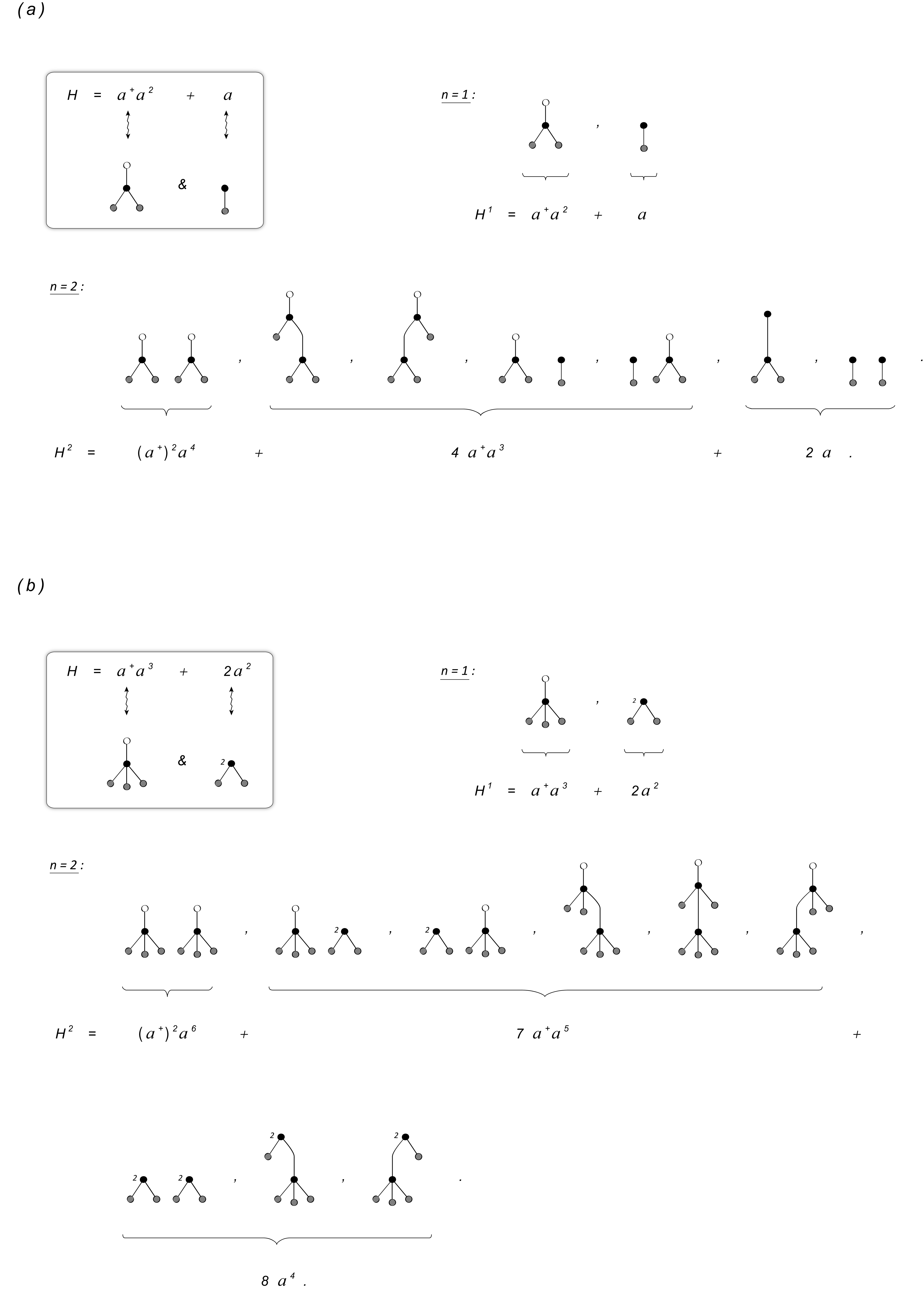
Figure 1: Building blocks (in the inset) and the associated graphs of order $n=1,2$ for Laguerre derivatives: (a) $H=D(1,1)=a^{{\dagger}}a^{2}+a$ and (b) $H=D(2,1)=a^{{\dagger}}a^{3}+2a^{2}$.

One should compare these “graphical results” with the explicit formulas of Eqs.(27) and (25) or the expansion coefficients of the generating function in Eq.(36) for $r=1,2$ and $M=1$. Thus, using Eq.(33), the coefficients multiplying the operators in Fig.(1a) are the first two terms in $B^{(1)}_{1}(n)=2,7,34,209$ for $n=1,2,\ldots$ (A002720). Similar coefficients in Fig.(1b) are the first two terms in $B^{(1)}_{2}(n)=3,16,121,1179$ for $n=1,2,\ldots$ (A121629).

5 Examples

1. For $r=M=1$, i.e. for $D(1,1)=aa^{\dagger}a$  one obtains (see [31] for a similar calculation):

$$\left[D(1,1)\right]^{n}=n!:L_{n}(-a^{\dagger}a):a^{n},$$ (40)

where $L_{n}(y)$ are Laguerre polynomials and Eq.(40) is derived from Eq.(39) and using the definition of $L_{n}(y)$ via the function $\ {}_{1}F_{1}$. Then

$$\begin{array}[]{rcl}e^{\lambda D(1,1)}&=&{\displaystyle\sum_{n=0}^{\infty}\frac{\lambda^{n}}{n!}\left[{D(1,1)}\right]^{n}=}\\ &=&{\displaystyle\ :\sum_{n=0}^{\infty}L_{n}(-a^{\dagger}a)(\lambda a)^{n}:\ =\ :\frac{1}{1-\lambda a}\exp\left(\frac{\lambda a^{\dagger}a^{2}}{1-\lambda a}\right):\ ,}\end{array}$$ (41)

where in Eq.(41) we have used the ordinary generating function for the Laguerre polynomials [5].

Using other generating functions listed on p.704 of Ref.[5] one can derive further formulas of type Eq.(41). ( In a) and b) below: $\lambda\neq 0,\ p=1,2,...$).

a) Formula $5.11.2.6$ of [5] for $\alpha=0$ provides the normal ordering of

$${}_{1}F_{1}\left([b],[1],\lambda D(1,1)\right)={\displaystyle:\!\frac{1}{(1-\lambda a)^{b}}{{}_{1}F_{1}}\left([b],[1],\frac{\lambda a^{{\dagger}}a^{2}}{1-\lambda a}\right)\!:\ ,}$$ (42)

which for $b$ integer and half-integer can be written down in terms of known functions. Examples are:

$${\hskip-19.0pt}\begin{array}[]{l}\hskip-50.0pt{{{}_{1}{F}_{1}}\left([3],[1],\lambda D(1,1)\right)={\displaystyle:\!\frac{1}{(1-\lambda a)^{3}}L_{2}\left(-\frac{\lambda a^{{\dagger}}a^{2}}{1-\lambda a}\right)\exp{\left(\frac{\lambda a^{{\dagger}}a^{2}}{1-\lambda a}\right)}\!:\ ,}}\\ \\ \hskip-50.0pt{{{}_{1}{F}_{1}}\left([\frac{3}{2}],[1],\lambda D(1,1)\right)={\displaystyle:\exp{\left(\frac{\lambda a^{{\dagger}}a^{2}}{2(1-\lambda a)}\right)}\times}}\\ \\ \hskip 78.0pt{\displaystyle{\times\left[I_{0}\left({\frac{\lambda a^{{\dagger}}a^{2}}{2(1-\lambda a)}}\right)(1+\frac{\lambda a^{{\dagger}}a^{2}}{1-\lambda a})+I_{1}\left({\frac{\lambda a^{{\dagger}}a^{2}}{2(1-\lambda a)}}\right)\right]\!:\ .}}\end{array}$$ (43)

where $I_{0}(y)$ and $I_{1}(y)$ are modified Bessel functions.

b) Similarly, we consider the formula $5.11.2.8$ of [5]:

$$\sum_{n=0}^{\infty}\left(\begin{array}[]{c}{n+p}\\ {n}\end{array}\right)t^{n}L_{n+p}(x)=\frac{1}{(1-t)^{p+1}}e^{-\frac{tx}{1-t}}L_{p}\left({\frac{x}{1-t}}\right)\ .$$ (46)

Using Eq.(40) we obtain the normally ordered form of $[\lambda D(1,1)]^{p}\exp(\lambda D(1,1))/p!\,$:

$$\begin{array}[]{rcl}{\displaystyle\frac{1}{p!}\sum_{n=0}^{\infty}\frac{[\lambda D(1,1)]^{n+p}}{n!}}&=&{\displaystyle\sum_{n=0}^{\infty}\frac{(n+p)!}{p!n!}:L_{n+p}(-a^{\dagger}a)(\lambda a)^{n+p}:\ =}\\ &=&{\displaystyle:\frac{1}{(1-\lambda a)^{p+1}}e^{\frac{\lambda a^{\dagger}a^{2}}{1-\lambda a}}L_{p}(-\frac{a^{\dagger}a}{1-\lambda a}):\ (\lambda a)^{p}\ .}\end{array}$$ (47)

2. The normal order of the modified Bessel function of the first kind $I_{0}\left(2(\lambda D(1,1))^{1/2}\right)$ may be derived:

$$\begin{array}[]{rcl}I_{0}(2(\lambda D(1,1))^{1/2})&\!=\!&\!{\displaystyle:\sum_{n=0}^{\infty}\frac{L_{n}(-a^{\dagger}a)(\lambda a)^{n}}{n!}:=}\\ &\!=\!&\!{\displaystyle:e^{\lambda a}J_{0}(2\sqrt{\lambda(-aa^{\dagger}a)}):\ =\ :e^{\lambda a}I_{0}(2\sqrt{\lambda a^{\dagger}a^{2}}):\ ,}\end{array}$$ (48)

where in the last line we have used the exponential generating function of Laguerre polynomials [5]. The analogous formula for $J_{0}\left(2(\lambda D(1,1))^{1/2}\right)$ reads

$$\begin{array}[]{rcl}J_{0}(2(\lambda D(1,1))^{1/2})&=&{\displaystyle\ :\sum_{n=0}^{\infty}\frac{L_{n}(-a^{\dagger}a)(-\lambda a)^{n}}{n!}:}=\\ &&{\displaystyle=\ :e^{-\lambda a}I_{0}(2\sqrt{\lambda a^{\dagger}a^{2}}):\ .}\end{array}$$ (49)

3. We quote here the eigenfunctions of $D_{x}(r,M)$ with eigenvalue 1 satisfying $D_{x}(r,M)E(r,M;x)=E(r,M,x)$, with the following $r$ boundary conditions:

$$E(r,M;0)=1,\ \ \ \ \ \ \ \left.\left[\frac{d^{p}}{{dx}^{p}}E(r,M;x)\right]\right|_{x=0}=0,\ \ \ p=1,\dots,r-1$$ (50)

which are

$$E(r,M;x)=\ _{0}F_{M+r-1}([\;\;],[\underbrace{1/r,2/r,...,(r-1)/r,}_{{r-1}\ times}\underbrace{1,...,1}_{M\ times}],x^{r}/r^{r+M})\ .$$ (51)

Useful normal ordering formulas can be obtained by applying the Dobiński relations to the eigenfunctions of $D_{x}(1,M)$ with the argument taking operator values, see Eq.(51), i.e. $E(1,M;D_{x}(1,M))$. We briefly show the calculation, in boson notation, for $E(1,2;\lambda D(1,2))=_{0}\!\!F_{2}([\;\;],[1,1],\lambda D(1,2))$, see Eq.(39) :

$$\begin{array}[]{l}{}_{0}F_{2}([\;\;],[1,1],\lambda D(1,2))=\sum\limits_{n=0}^{\infty}{\displaystyle\frac{\lambda^{n}}{(n!)^{3}}}[a(a^{\dagger}a)^{2}]^{n}=\\ \\ =\ :e^{-a^{\dagger}a}\sum\limits_{l=0}^{\infty}{\displaystyle{\frac{(a^{\dagger}a)^{l}}{l!}}}\sum\limits_{n=0}^{\infty}{\displaystyle\frac{((n+l)!)^{2}}{(l!)^{3}}}(\lambda a)^{n}:\ =\\ \\ =\ :e^{-a^{\dagger}a}\sum\limits_{l=0}^{\infty}{\displaystyle\frac{(a^{\dagger}a)^{l}}{l!}}\ _{2}F_{2}([1+l,1+l],[1,1],\lambda a):\ ,\end{array}$$ (52)

and similarly

$$\begin{array}[]{l}E(1,M;\lambda D(1,M))=\ _{0}F_{M}([\;\;],[\ \underbrace{1,1,...1}_{M\ times}\ ],\lambda D(1,M))=\\ ={\displaystyle\ :e^{-a^{\dagger}a}\sum_{l=0}^{\infty}\frac{(a^{\dagger}a)^{l}}{l!}\ _{M}F_{M}([\ \underbrace{1+l,1+l,...,1+l}_{M\ times}\ ],[\underbrace{1,1,...,1}_{M\ times}],\lambda a):\ ,}\end{array}$$ (53)

which indicates a pattern appearing in the course of this procedure.

Indeed, by evaluating the coherent state expectation value of Eq.(53) between $\langle z=1|\dots|z=1\rangle$ in the spirit of Eq.(16) we obtain the hypergeometric generating functions of the numbers $B^{(M)}_{1}(n)$ as then

$$\begin{array}[]{l}{\displaystyle e^{-1}\sum\limits_{l=0}^{\infty}\frac{1}{l!}\ _{M}F_{M}([\underbrace{l+1,l+1,\dots,l+1}_{M\ times}],[\underbrace{1,1,...1}_{M\ times}],\lambda)=}\\ ={\displaystyle\sum_{n=0}^{\infty}B^{(M)}_{1}(n)\frac{\lambda^{n}}{(n!)^{M+1}},\ \ \ \ \ M=1,2,\dots\ .}\end{array}$$ (54)

The hypergeometric generating function of $B_{r}^{(M)}(n,x)$ for arbitrary $r$ and $M$ can also be obtained from Eq.(25), and reads:

$$\begin{array}[]{l}{\displaystyle e^{-x}\sum\limits_{l=0}^{\infty}\frac{x^{l}}{l!}\ _{M}F_{M}([\underbrace{l/r+1,l/r+1,\dots,l/r+1}_{M\ times}],[\underbrace{1,1,...1}_{M\ times}],r^{M}\lambda)=}\\ {\displaystyle=\sum_{n=0}^{\infty}B^{(M)}_{r}(n,x)\frac{\lambda^{n}}{(n!)^{M+1}}\ .}\end{array}$$ (55)

In spite of their apparent complexity the l.h.s of the above equations can be straightforwardly handled by computer algebra systems [32].

6 Conclusions and outlook

We have found exact analytical expressions for the generalized Stirling numbers and generalized Bell polynomials which appear in the normal ordering of powers of Laguerre-type derivative operators, and have provided a complete set of hypergeometric generating functions for these quantities. The combinatorial aspect of the problem was demonstrated by finding an exact mapping between the normal ordering and an enumeration of increasingly labelled, multivertex forests constructed according to a two-parameter $(r,M)$ prescription. In this way analytical, numerical and combinatorial facets of this problem have been given a very complete treatment. We have also used generalized Dobiński relations to investigate the properties of these Laguerre-type differential operators. We provided a large number of operational formulas involving functions of Laguerre derivatives, which can alternatively be applied using the boson language. The framework developed above enables one to construct and analyze new coherent states relevant to nonlinear quantum optics, which will be the subject of forthcoming research.

7 Acknowledgments

We wish to acknowledge support from Agence Nationale de la Recherche (Paris, France) under programme no. ANR-08-BLAN-0243-2. Two of us, P.B. and A.H., wish to acknowledge support from the Polish Ministry of Science and Higher Education under grants no. N202 061434 and 202 107 32/2832.

8 Appendix: Sheffer-type operators

We derive Eq.(35) with the help of methods developed in Ref.[8]. First, observe that $D(r,1)=a^{\dagger}a^{r+1}+ra^{r}$ from which it follows that $D^{\dagger}(r,1)=(a^{\dagger})^{r+1}a+r(a^{\dagger})^{r}$ is an operator of Sheffer-type: $D^{\dagger}(r,1)=v(a^{\dagger})+q(a^{\dagger})a$ with $q(x)=x^{r+1}$ and $v(x)=rx^{r}$. The normally ordered form of $\exp(\lambda D^{\dagger}(r,1))$ is obtained by solving the linear differential equations (Eqs.(2) and (3) of Ref.[8]) for $T(\lambda,x)$ and $g(\lambda,x)$ yielding

$$T(\lambda,a^{\dagger})=\frac{a^{\dagger}}{(1-\lambda r(a^{\dagger})^{r})^{1/r}},{\hskip 207.0pt{(A1)}}$$

and

$$g(\lambda,a^{\dagger})=\frac{1}{1-\lambda r(a^{\dagger})^{r}}\ .{\hskip 230.0pt{(A2)}}$$

According to Eq.(29) of [8] the normally ordered form of $e^{\lambda D(r,1)}$ is

$$e^{\lambda D(r,1)}=\left[e^{\lambda D^{\dagger}(r,1)}\right]^{\dagger}=\ :g(\lambda,a)e^{a^{\dagger}(T(\lambda,a)-a)}:{\hskip 121.0pt{(A3)}}$$

which gives Eq.(35).

References

References

• [1] G.Dattoli and P.Ricci, Georgian Math. J. 10, 481 (2003).
• [2] G.Dattoli, P.E.Ricci and I.Khomasuridze, Int. Transf. and Spec. Funct. 15, 309 (2004).
• [3] G.Dattoli, M.R.Martinelli and P.E.Ricci, Int. Transf. and Spec. Funct. 16, 661 (2005).
• [4] N.Fleury and A.V.Turbiner, J. Math. Phys. 35, 6144 (1994).
• [5] A.P.Prudnikov, Yu.A.Brychkov and O.I.Marichev, Integrals and Series, v.2: Special functions (Gordon and Breach, New York, 1998).
• [6] G.Dattoli, A.M.Mancho, M.Quatromini and A.Torre, Radiation Phys. Chem. 61 99 (2001).
• [7] G.Dattoli, P.L.Ottaviani, A.Torre and L.Vásquez, Riv. Nuovo Cim. 20, serie 4 no.2, 1 (1997).
• [8] P.Blasiak, A.Horzela, K.A.Penson, G.H.E.Duchamp and A.I.Solomon, Phys. Lett. A 338, 108 (2005).
• [9] J.R.Klauder and E.C.G.Sudarshan, Fundamentals of Quantum Optics (Benjamin, New York, 1968); J.R.Klauder and B-S.Skagerstam, Coherent States. Application in Physics and Mathematical Physics (World Scientific, Singapore, 1985).
• [10] R.L.Matos Filho and W.Vogel, Phys. Rev. A 54 4560 (1996).
• [11] M.Rasetti, J.Katriel, A.I.Solomon and G.D’Ariano, in Squeezed and Nonclassical Light, P.Tombesi and E.P.Pike Eds., ( Plenum, New York, 1989) p. 301
• [12] A.I.Solomon, Phys. Lett. A188, 215 (1994).
• [13] L.Comtet, Advanced Combinatorics (Reidel, Dordrecht, 1974).
• [14] E.W.Weisstein, “Stirling Number of the First Kind”, from MathWorld–A Wolfram Web Resource, http://mathworld.wolfram.com/StirlingNumberoftheFirstKind.html.
• [15] P.Blasiak, K.A.Penson and A.I.Solomon, Phys. Lett. A 309, 198 (2003).
• [16] P.Blasiak, K.A.Penson and A.I.Solomon, Ann. of Comb. 7, 127 (2003).
• [17] P.Blasiak, K.A.Penson, A.I.Solomon, A.Horzela and G.H.E.Duchamp, J. Math. Phys. 46, 052110 (2005).
• [18] M.A.Méndez, P.Blasiak and K.A.Penson, J. Math. Phys. 46, 083511 (2005).
• [19] W.H.Louisell, Quantum Statistical Properties of Radiation (Wiley, New York, 1990).
• [20] P.Blasiak, A.Horzela, K.A.Penson, A.I.Solomon and G.H.E.Duchamp, Am.J.Phys. 75, 639 (2007); this pedagogical paper contains exhaustive list of references dealing with the boson normal ordering problem.
• [21] J.Katriel, Lett. Nuovo Cim. 10, 565 (1974).
• [22] K.E.Cahill and R.J.Glauber, Phys. Rev. 177, 1857 (1969); the formula is attributed to J.Schwinger.
• [23] V.V.Mikhailov, J. Phys. A : Math. Gen. 16, 3817 (1983); J. Katriel, J. Phys. A : Math. Gen. 16, 4171 (1983).
• [24] P.Blasiak, K.A.Penson and A.I.Solomon, J. Phys. A: Math. Gen. 36, L273 (2003).
• [25] P.Blasiak, A.Horzela, K.A.Penson and A.I.Solomon, J. Phys. A: Math. Gen. 37, 4999 (2006).
• [26] N.J.A.Sloane, Encyclopedia of Integer Sequences, http://www.research.att.com/~njas/sequences, (2009).
• [27] A.V.Turbiner and G.Post, J. Phys. A: Math. Gen. 27, L9 (1994).
• [28] P.Blasiak and A.Horzela, arXiv:0710.0266.
• [29] P.Blasiak, A.Horzela, K.A.Penson, A.I.Solomon and G.H.E.Duchamp, J. Phys. A: Math. Gen. 41, 415204 (2008).
• [30] P.Flajolet and R.Sedgewick, Analytic Combinatorics (Cambridge University Press, 2008).
• [31] J.Riordan, Combinatorial Identities (Wiley, New York, 1968).
• [32] We have made extensive use of Maple in this paper.