Nonextensive thermal sources of cosmic rays

Abstract

The energy spectrum of cosmic rays (CR) exhibits power-like behavior with a very characteristic ”knee” structure. We consider a possibility that such a spectrum could be generated by some specific nonstatistical temperature fluctuations in the source of CR with the ”knee” structure reflecting an abrupt change of the pattern of such fluctuations. This would result in a generalized nonextensive statistical model for the production of CR. The possible physical mechanisms leading to these effects are discussed together with the resulting chemical composition of the CR, which follows the experimentally observed abundance of nuclei.

I Introduction

The energy spectrum of cosmic rays (CR) has characteristic power-like behavior with a ”knee” structure (plus some other less prominent features) and remains constantly matter of hot debate (see CR-origin and references therein). It could reflect the action of different regimes of diffusive propagation of CR in the Galaxy combined with its different chemical composition, but it could also be due to some, so far unspecified, property of the production processes within the source of the CR itself. In this work we shall consider this possibility assuming that CR are produced following a generalized nonextensive thermal approach Tsallis ; WWTq . Actually, nonextensive statistical mechanics Tsallis has been applied to CR before: in previous1 the ”knee” structure was attributed to the crossover between the assumed fractal-like thermal regimes of CR propagation (characterized by different temperatures $T$ and nonextensive parameters $q$), whereas in previous2 the possible nonextensive thermal features of CR flux have been investigated but only up to the ”knee” region, the origin of which was not discussed. In both cases the obtained values of temperatures were much too high to be accommodated by any known physical mechanism. In this paper we propose a mechanism which is apparently capable to describe the whole spectrum of CR, including the ”knee” region, using physically reasonable values of temperature of the source of CR. The observed power-like behavior of the energy spectrum of CR is attributed (as in previous2 ) to fluctuations of the temperature in the source producing CR and the occurrence of ”knee” (cf., Fig. 1a) is connected with some abrupt change of this fluctuation pattern WW , visualized by a dramatic change in the nonextensivity parameter observed Fig. 1b. However, to keep the temperature of the CR source acceptably low, one has to allow additionally for energy transfer to the production region; this is assumed to proceed through the mechanism proposed in WWTq and is characterized by some effective temperature $T_{eff}$ . These points summarize what we call a generalized nonextensive thermal approach (GNTA), which we shall now describe in more detail.

It must be stressed at this point that, for the sake of clarity of presentation, we consider in what follows only a very simplified situation. Namely, we assume that GNTA is, for a moment, the only mechanism of production of the CR present. It must be realized that in reality GNTA would have to be incorporated into many other possibilities considered in the usual analysis of CR (and listed, for example, in CR-origin ).

The organization of our paper is as follows. In the next Section we present some basic considerations concerning nonextensive statistics and CR, out of which the discussion of the chemical composition of CR seen from that point of view is a new element here. Section III contains our results and their physical interpretation in terms of some specific properties in the superfluid stages of neutron stars supplied by the proposition of introducing phenomenologically the energy transfer to CR (described by some effective temperature $T_{eff}$ and needed to assure the consistency of obtained parameters). In Section IV we discuss the influence of acceleration and propagation of CR on energy spectra and composition. A summary and concluding remarks are presented in Section V.

II Basic elements of nonextensive statistics and Cosmic Rays

II.1 Generalities

Nonextensive statistical mechanics as proposed and developed in Tsallis is based on the generalized entropy functional (Tsallis entropy),

$$S_{q}\,=\,-\frac{\int dE\,P^{q}(E)\,-\,1}{q-1}\,\,.$$ (1)

Its maximization under appropriate constrains yields a characteristic power-like distribution ($q$-exponential distribution, $\exp_{q}(\dots)$):

$$P_{q}(E)=\frac{2-q}{T}\exp_{q}\left(-\frac{E}{T}\right)=\frac{2-q}{T}\,\left[1-(1-q)\frac{E}{T}\right]^{\frac{1}{1-q}}.$$ (2)

For $q\rightarrow 1$ one recovers the usual Boltzmann-Gibbs-Shannon (BGS) entropy and the usual exponential distribution. This equilibrium distribution can alternatively be obtained by solving the following differential equation,

$$\frac{dP(E)}{dE}=-\frac{P^{q}(E)}{T}.$$ (3)

The extended version of this equation with two terms (accommodating two different values of $q$ and $T$) has been used with apparent success in previous1 to describe the flux of CR. The ”knee” appears there as a crossover between two fractal-like thermal regimes characterized by $(T,q)$ and $(T^{\prime},q^{\prime})$. However, the values of temperatures obtained there ($(T,T^{\prime})\sim 100\div 1000$ MeV) are uncomfortably high and cannot be attributed to any known mechanism of CR production.

On the other hand, there is growing evidence that a nonextensive formalism applies most often to nonequilibrium systems with a stationary state that possesses strong fluctuations of the inverse temperature parameter $\beta=1/T$ WW ; Biro (cf., also Add ). In fact, fluctuating $\beta$ according to gamma distribution (cf. Eq. (9) below) with variance $Var(\beta)$ results in a power like distribution (2) with the deviation of the nonextensivity parameter $q$ from unity being given by the strength of these fluctuations,

$$q-1\,=\,\frac{Var(\beta)}{\langle\beta\rangle^{2}}.$$ (4)

This observation was used in previous2 to describe the energy spectrum (but only up to the ”knee” region). Again, although the results were reasonably good the estimated temperature $T\sim 170$ MeV is far too high. This was because the author insisted on the description of the whole range of energy spectrum up to the ”knee” region, including its very low energy part, which is, however, governed mainly by the geomagnetic cut-off and diffusion effects and should therefore be considered separately (it is thus not covered by our approach).

II.2 Energy spectrum

Treating CR as relativistic particles (for which rest mass $m$ can be neglected) their energy is $E\sim p$ and the density of states is that of an ideal gas in three dimensions, $\Omega(E)\propto E^{2}$. The corresponding energy spectrum $\Phi(E)$ is then

$$\Phi(E)\,=\,N_{0}\,E^{2}\,P(E),$$ (5)

where $N_{0}$ is normalization factor. For $P(E)$ given by Eq. (2) we have, for $E>>T$, power spectrum

$$\Phi(E)\propto E^{-\gamma};\qquad\gamma=\frac{3-2q}{q-1}.$$ (6)

As seen in Fig. 1a it changes in the region named ”knee” where the slope $\gamma_{1}\simeq 2.7$ at energies below $\sim 10^{15}$ eV and $\gamma_{2}\simeq 3.1$ above it. In the language of the nonextensivity parameters it would mean that $q_{1}=1.213$ before and $q_{2}=1.196$ after the ”knee”. For $q$ understood as a measure of fluctuations, as it is the case in our paper, one therefore witnesses at the ”knee” a change of fluctuation pattern.

Figure 1: (Color online) $(a)$ Schematic view of the observed CR energy spectrum CR-origin with characteristic features clearly indicated. $(b)$ The pattern of fluctuations obtained from the above by means of nonextensive statistics approach and represented by the heat capacity $C_{V}$ as given by Eq. (11) (see text for details). Notice that previous irregularities are now dramatically enhanced.

II.3 The chemical composition

If the energy distribution of CR follows the Tsallis formula (2), it is natural to expect that also the abundance of nuclei with mass $A$ will follow the same pattern. We therefore expect that

$$\omega(A)\propto\left[1-(1-q)\frac{A\varepsilon}{T}\right]^{\frac{1}{1-q}},$$ (7)

where $\varepsilon$ is the average energy of nucleon equal to $\varepsilon=\frac{3}{5}E_{F}$. The typical value of the Fermi energy for nucleus consisting of $A$ nucleons (distributed in sphere of radius $R=1.25A^{1/3}$) is $E_{F}\simeq 30$ MeV, it means then that $\varepsilon\simeq 22$ MeV. In Fig. 2 we show $\omega(A)/\omega(A=1)$ for $\varepsilon=22$ MeV and $T=100$ MeV as function of $A$ for two values of $q$: $q=1.2$ and $q=1.15$. As one can see the sensitivity to $q$ is rather weak . The average mass number (for the spectrum $\omega(A)$) is

$$\langle A\rangle=\frac{2-q+T/\varepsilon}{3-2q}.$$ (8)

Numerically evaluated $\langle\ln(A)\rangle$ equals $1.82$ below the ”knee” (for greater $q$) and $1.78$ above the ”knee” (for smaller $q$) and shows that predicted changes of chemical composition (due to changes of spectral index) in the ”knee” region are negligible. Notice that the upper limit estimation for the usual BG distribution (corresponding to $q=1$ here) leaves the majority of points for large values of $A$ well above the curve. From this point of view our prediction is much better (although, the thermal model alone is already able to provide quite reasonable chemical composition of CR) .

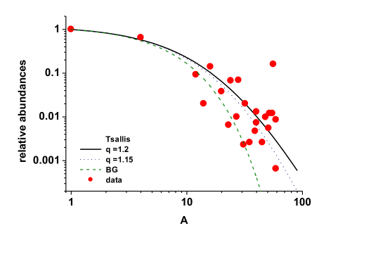
Figure 2: (Color online) The chemical composition of CR (relative to hydrogen at $1$ TeV) corresponding to nonenextensive picture advocated in this work. Data points are from Abundances .

One should keep in mind that the relative dissemination of nuclides shows many intriguing features which should be connected with specific properties of nuclei, cf., for example, properties . We close this section by stressing that our $\omega(A)$ as given by Eq. (7) (and therefore represented by a continuous curve) does not account for any differences between nuclei. In fact, it even does not describe the abundance in the source. It describes only the emissive power of thermal source and shows that this factor (neglecting differences between particular nuclei) determines the global characteristics of the observed spread of nuclides.

III Results

III.1 Temperature fluctuations

As mentioned above, the special role in converting an exponential distribution to its $q$-exponential counterpart play fluctuations of the inverse temperature $\beta$ described by a gamma function WW ; Add ,

$$f(\beta)=\frac{\mu}{\Gamma(\nu)}\left(\mu\beta\right)^{\nu-1}\,\exp\left(-\beta\mu\right)$$ (9)

where $\mu^{-1}=\beta_{0}(q-1)$ and $\nu^{-1}=q-1$. There are a priori at least two scenarios leading to such $f(\beta)$: $(i)$ one can have many sources with different temperatures, the number of which is distributed that way or $(ii)$ one can have temperature fluctuations in small parts of a source. The first possibility is, however, rather unlikely because in this case either one would have to accept sources with unphysically large and small temperatures or else use the temperature distribution in some limited domain, i.e., work with a truncated version of gamma distribution. This, however, would result in a very characteristic rapid break in the energy spectrum. This is not observed in the experiment.

We shall therefore concentrate on the second possibility. To illustrate it, suppose one has a thermodynamic system, different small parts of which have locally different temperatures, i.e., its temperature understood in the usual way fluctuates. Let $\xi(t)$ describes the stochastic changes of temperature in time and let it be defined by the white Gaussian noise ($\langle\xi(t)\rangle=0$ and $\langle\xi(t)\xi(t+\Delta t)\rangle=2D\delta(\Delta t)$). The inevitable exchange of heat which takes place between the selected regions of our system leads ultimately to an equilibration of temperature and, as shown in WW , the corresponding process of heat conductance eventually leads to the gamma distribution (9) mentioned before with variance (4) related to the heat capacity $C_{V}$ of this system (expressed in units of Boltzmann constant $k_{B}$, which we put equal unity in what follows) by S

$$\frac{Var(\beta)}{<\beta>^{2}}=\frac{1}{C_{V}}$$ (10)

and we have finally that

$$C_{V}=\frac{1}{q-1}=\gamma+2,$$ (11)

where we have used Eq. (6) connecting the spectral index $\gamma$ of the energy spectrum with the nonextensivity parameter $q$. In this way, we come directly to the possible physical interpretation of the nonextensivity parameter which allows us to translate the pattern observed in Fig. 1a into that shown in Fig. 1b. Here $C_{V}$, as given by Eq. (11), is shown as a function of energy at which we observe the essential influence of given $C_{V}$ on the slope of energy spectrum. As will be discussed in detail below in Sec. III.2, although $C_{V}$ as such is energy independent it can change with temperature $T$ in the source and changes abruptly at some temperature $T_{c}$ (identified, for example, with $T_{cut}$ in Sec. III.2). These changes of $C_{V}$ result in changes of the slope of the observed energy spectrum at $E\sim 2T_{c}$).

To summarize this part: In what follows, we shall concentrate mainly on the change of fluctuation pattern in the ”knee” region and we shall argue that it could indicate an abrupt change in the heat capacity in the source of CR of the order of $C_{2}/C_{1}=1.09$. Notice that this change is much more pronounced and dramatic than the corresponding change of slope in the ”knee” region observed in Fig. 1a.

III.2 Possible physical interpretations of the fluctuation pattern

Can one expect something of this kind to happen in the astrophysical environment of the CR? In what follows we shall argue that, indeed, one can. Let us first notice that the subject of temperature fluctuations in astrophysics is a much-discussed problem nowadays. Its effect on the temperatures empirically derived from spectroscopic observations was first investigated in P whereas in 13a ; 13b ; 13c ; 13d it was shown that temperature fluctuations in photoionized nebulea have great importance to all abundance determinations in such objects. This means that discussion of the heat capacity or, equivalently, the behavior of the parameter $q$ defining the energy spectrum, is fully justified. In what follows we shall concentrate on the problem of the heat capacity of astrophysical objects, in particular in neutron stars, concentrating on some peculiarities connected with their description in terms of Fermi liquids.

We start with fluid/superfluid transitions in such systems and their effect on the heat capacity. In neutron stars one observes the following feature. The total specific heat of their crust, $C$, is the sum of contributions from the relativistic degenerate electrons, from the ions and from degenerate neutrons. In the temperature that can be reached in the crust of an accreting neutron star (which is of the order of $T\sim 5\cdot 10^{8}$ K and is below the Debaye temperature $T_{D}\sim 5\cdot 10^{9}$ K) we have $C_{ion}<C_{e}<C_{n}$. When the temperature drops below the critical value $T=T_{C}$ the neutrons become superfluid and their heat capacity $C^{sf}_{n}$ increases HC1 ; HC2 ,

$$\frac{C^{sf}_{n}}{C_{n}}\simeq 3.15\frac{T_{C}}{T}\exp\left(-1.76\frac{T_{C}}{T}\right)\cdot\left[2.5-1.66\left(\frac{T}{T_{C}}\right)+3.68\left(\frac{T}{T_{C}}\right)^{2}\right].$$ (12)

At $T\sim 0.7T_{C}$ we have $C^{sf}_{n}\sim 1.1C_{n}$ what corresponds to the changes of spectral index by $\Delta\gamma\sim 0.5$. To summarize: one witnesses here an abrupt change in the heat capacity at some temperature, i.e., a phenomenon we were looking for.

The above example tells us that it is reasonable to expect the abrupt change of the specific heat in the CR source. Assuming that this really happens and taking seriously the apparent connection between $C_{V}$ and $q$ expressed by Eq. (11), we are lead to the natural conjecture that in this case the usual fluctuation pattern given by the gamma distribution (9) should be modifying accordingly. It is then assumed to be done by replacing Eq. (9) by its slightly modified version, characterized by two nonextensivity parameters, $q_{1}$ (acting before some temperature $T_{cut}$) and $q_{2}$ (acting after $T_{cut}$). The change $q_{1}\rightarrow q_{2}$ at $T_{cut}$ is assumed to be abrupt and the temperature $T_{cut}$ becomes a new parameter in our description. Following our proposition one obtains the following flux of CR:

$$\Phi(E) = N_{0}E^{2}\left[\int_{0}^{1/T_{cut}}e^{-\beta E}f_{q_{1}}(\beta)d\beta+\int_{1/T_{cut}}^{\infty}e^{-\beta E}f_{q_{2}}(\beta)d\beta\right]=$$ (13)

$$= N_{0}\,E^{2}\cdot\left[P_{q_{1}}(E)-\alpha_{1}(E)P_{q_{1}}(E)+\alpha_{2}(E)P_{q_{2}}(E)\right],$$

where $P_{q_{i}}(E)$ are given by Eq. (2) and

$$\alpha_{i}=\frac{\int_{1/T_{cut}}^{\infty}e^{-\beta E}f_{q_{i}}(\beta)d\beta}{\int_{0}^{\infty}e^{-\beta E}f_{q_{i}}(\beta)d\beta}=\frac{1}{\Gamma\left(\frac{1}{q_{i}-1}\right)}\Gamma\left[\frac{1}{q_{i}-1},\,\frac{1-\left(1-q_{i}\right)E/T}{\left(q_{i}-1\right)T_{cut}/T}\right].$$ (14)

Our results are presented in Fig. 3 where $q=1.214$ in Fig. 3a whereas in Fig. 3b $q_{1}=1.214$ and $q_{2}=1.2$; in both cases $T=100$ MeV. Notice that now we do not have a spectrum where, as in Section II.2, we change the value of $q$ at some energy $E_{c}$ to get the observed structure. Spectrum (13) is obtained by changing $q$ at some temperature $T_{cut}$ (i.e., by changing slightly the shape of gamma function (9)), this means that each $q$ gives a spectrum for all energies. For this reason the parameters $q$ here have slightly different values from these in Section II.2. With spectrum given by Eq. (13) the ”knee” region is reproduced very well, however, the price to be paid is the need of a suitable choice of temperature at which the fluctuation pattern changes (which amounts to assume the value of $T_{cut}\approx 10^{15}$ eV $\approx 10^{19}$ K) .

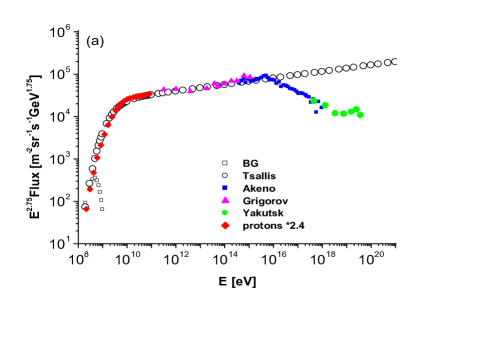
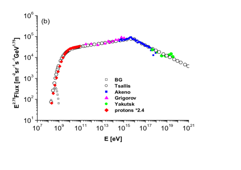
Figure 3: (Color online) $(a)$ CR energy spectra fitted by the single Tsallis distribution with $q=1.214$ and $T=100$ MeV. Notice the total inadequacy of a simple exponential (Boltzman, denoted by BG here) distribution in description of these spectra. $(b)$ The CR energy spectrum fitted by the double Tsallis distributions discussed in text, cf. Eqs. (13) and (14). It was obtained for $T=100$ MeV and assuming that fluctuations of the temperature change abruptly at $T_{cut}\approx 10^{15}$ eV $\approx 10^{19}$ K from $q=1.214$ to $q=1.2$. Data are from SPS , cf. also CR-origin .

The above mechanism is only able to describe the ”knee” region. To describe all details seen in Fig. 1b let us consider an other feature of heat capacity in Fermi liquids, namely its dependence on the effective mass of nucleons consisting such liquid. Following HC1 the proton heat capacity is proportional to the ratio of the effective mass of the proton in the neutron fluid to the mass of the free proton, $C\sim m^{*}/m$. In the case of a mixture of Fermi liquids the proton effective mass $m^{*}$ is affected by interactions with neutrons and other protons and is given by

$$\frac{m^{*}}{m}=1+\frac{1}{3}D_{p}\left[f^{pp}_{1}+\left(\frac{k_{F_{n}}}{k_{F_{p}}}\right)^{2}f_{1}^{pn}\right],$$ (15)

where $D_{p}$ denotes the density of quasiparticle states at the Fermi surface given by wave vectors $k_{F_{n}}$ and $k_{F_{p}}$ for, respectively, neutrons and protons, whereas $f^{pp}_{1}$ and $f^{pn}_{1}$ are Landau parameters BJK . Fig. 1b can then be interpreted as showing changes of $C$ with energy in the Fermi liquid. We start with the superfluid liquid with $C_{1}=4.7$ (here $m^{*}$ represents effective mass for $pp$ and $pn$ interactions), when energy increases we stop to see nuclear interactions and $C_{2}=5.1$ (with $m^{*}$ representing $pp$ interactions only), finally, for large $T$, one has the Fermi gas with $C_{3}=5.3$ and, still further, the usual Fermi liquid . Notice that

$$\frac{1}{3}D_{p}f_{1}^{pp}=\frac{C_{2}-C_{3}}{C_{3}}~{}~{}~{}{\rm and}~{}~{}~{}\frac{1}{3}D_{p}\left(\frac{k_{F_{n}}}{k_{F_{p}}}\right)^{2}f_{1}^{pn}=\frac{C_{1}-C_{2}}{C_{3}},$$ (16)

this results in the following relation between Landau parameters,

$$\left(\frac{k_{F_{n}}}{k_{F_{p}}}\right)^{2}\frac{f_{1}^{pn}}{f_{1}^{pp}}=\frac{C_{1}-C_{2}}{C_{2}-C_{3}}=2.$$ (17)

In the case of a one-component Fermi liquid we have the well known identity, $m^{*}/m=1+F^{pp}_{1}/3$, where $F_{1}^{pp}=D_{p}f_{1}^{pp}$. From (17) we see that in a two-component Fermi liquid the quantity $1-m^{*}/m$ is $3$ times bigger (this is because the parameter $f_{1}$ which determines the interaction between quasiparticles is negative, resulting in smaller effective mass). From properties of excited states in nuclear matter ($Pb$ and neighboring nuclei SZR ) $F_{1}^{np}=-0.5\pm 0.25$. If $F_{1}^{nn}<F_{1}^{np}<F_{1}^{pp}$ and taking (after PH ) $F_{1}^{nn}-F_{1}^{pp}=-0.2$, we can estimate that for neutron-star matter one has $m^{*}/m=1+F_{1}^{pp}\simeq 1-0.4\pm 0.3=0.6\pm 0.3$.

III.3 The notion of the effective temperature $T_{eff}$

Let us now come back to the results presented in Fig. 3. Although a double Tsallis fit looks rather impressive there are two shortcomings which we shall now discuss in more detail. First is the fact that we still need a too high value of the temperature, $T=100$ MeV, which cannot be accommodated by any reasonable physical mechanism of production of CR’s. Second is the very high value of the $T_{cut}$ temperature where change in the fluctuation pattern is supposed to take place.

The possible way out of both dilemmas we are going to propose now is to keep the value of $T=100$ MeV but change its meaning. This can be done by adding to the mechanism proposed in WW (which was accounting only for the possible fluctuations of $T$) an additional effect of the possible viscosity which describes the possible transfer of energy between the region of production and surroundings (cf. WWTq and hi for details). As a result one gets the same power-like distribution as before but with the previous $T$ replaced by an effective temperature $T_{eff}$ :

$$T_{eff}=T_{0}+(q-1)T_{visc}.$$ (18)

Here $T_{0}$ is the temperature around which one has fluctuations and $T_{visc}$ is some new parameter depending on the transport properties of the surrounding space around the emission region.

A few words of explanation are necessary at this point. Following hi , in the case of heavy ion collisions, where this concept has been introduced for the first time, $T_{visc}=\eta f(u)/(Dc_{\rho}\rho)$, where $\eta f(u)$ presents the effect of a possible viscosity, with viscosity coefficient $\eta$ and $f(u)=\left(\frac{\partial u_{i}}{\partial x_{k}}+\frac{\partial u_{k}}{\partial x_{l}}\right)^{2}$ ($u$ being velocity), whereas $D$, $c_{\rho}$ and $\rho$ are, respectively, the strength of the temperature fluctuations, the specific heat under constant pressure and the density. Here this quantity is supposed to model the possible transfer of energy towards the CR particle. To estimate its value let us notice that $(q-1)T_{visc}\sim(\tau/\tau_{c})T_{0}$ where $\tau$ and $\tau_{c}$ are, respectively, a relaxation time of the corresponding dissipative process and the mean collision time. They have distinct physical meanings. Namely, $\tau$ is the time (in most cases macroscopic) taken by the system to spontaneously return to the steady state (whether in thermal equilibrium or not) after being suddenly removed from it. It is, to some extent connected to the mean collision time $\tau_{c}$ of the particles responsible for the dissipative process. There is no general formula linking them, their relationship depends in each case on the system and circumstances under consideration. In particular, $\tau$ is small for photon-electron and photon-photon interactions at room temperature ($\propto 10^{-11}$ and $\propto 10^{-13}$ seconds, respectively). In the case of neutron star, $\tau$ is of the order of the scattering time between electrons (which carry the heat) but this fact is not obstacle (no matter how large the mean free path of this electron may be) to consider the neutron star as formed by a Fermi fluid of degenerate neutrons. One finds in this case the relaxation times as large as $\tau\sim 10^{2}$ seconds (for $T\sim 10^{6}$ K, $\rho\sim 10^{14}$g/cm³ and $u\sim 10^{3}$ cm/s) 3star whereas in the degenerate core of aged stars $\tau$ can reach $1$ second 1star . The fact that $\tau$ can quantitatively greatly differ from $\tau_{c}$ is most dramatically suggested by the matter-radiation decoupling in the early universe (the relaxation time of shear viscosity turns out to be several order of magnitude larger than the collision time for most of the radiative era) 2star . For this region one can expect that $T_{visc}$ may be large enough (for example, $T_{visc}/T_{0}\sim 10^{8}$) to be a reasonably parameter describing the influence of surroundings on the CR particle. Therefore in such picture there are fluctuations of temperature $T$ characterized by the parameter $q$ and connected with the character of the source, for example, as discussed here, but there is also a surrounding space around the emission point which can pump energy into some selected region from which a CR particle is emitted. This is described by the positive parameter $T_{visc}$. As a result we are getting the total $T_{eff}$ that grows with $q$.

Our schematic view in what concerns the fate of the CR spectrum is then the following. $(i)$ CR are produced in an object where we have low temperature which experiences some fluctuations around $T=T_{0}$ given by $q>1$ (with $T_{0}$ of the order of MeV). Now $T_{0}$ can be as small as desired to properly fit the expected features of the CR source. $(ii)$ By introducing to the previous description WW some (so far unspecified) flow WWTq ; hi , the corresponding Tsallis distribution now has $T=T_{eff}$, which can be quite large for example, of the order of the observed $100$ MeV). $(iii)$ Therefore, in the spectrum of CR one observes a Tsallis distribution with $T_{eff}\sim 100$ MeV (as in the previous attempts previous1 ; previous2 ) but now it is not the temperature of the source of CR itself, but it is composed from the temperature of the CR’s source itself, $T_{0}$, and the effect of the action of the surrounding space which is given by $T_{visc}$. It should be stressed that such an effect appears only in the case of Tsallis distribution. Only for $q>1$ is $T_{eff}>T_{0}$. If there are no temperature fluctuations one always has $T_{eff}=T_{0}$.

Interestingly enough, the proposed mechanism seems to be capable also to alleviate the second problem, namely the uncomfortably high value of the $T_{cut}$ where the change of the nonextensivity parameter $q$ occurs. This is because, as discussed in And , when one considers viscosity effects in stars, one observes very large abrupt changes of the viscosity coefficient which can easily result in an effective $T_{visc}$ of the desired order to fit the parameter $T_{cut}$.

IV Propagation and sources of cosmic rays

Following previous1 one can argue that nonextensive approach represented by Eq. (2) can also be connected with the process of CR propagation. In our case such scenario would mean that parameter $T_{visc}$ in $T_{eff}$ can represent summarily some effective modelling of the propagation of CR. Whereas detailed discussion of such a possibility is outside the scope of the present paper, a few words on propagation of CR and its possible influence on the spectra and composition of CR are in order here.

So far we have considered only the sources of CR insisting on the possibility that they are of thermal but nonextensive type. We shall now address the possible influence on our results by the propagation of CR. Measurements of the composition and energy spectra of CR characterize the CR population after the observed particles have travelled from their production sites (i.e., the sources) through distant space towards the remote detectors. It is expected that both the composition of the particles and the shape of their energy spectra undergo in such process changes due to a variety of processes encountered during the propagation.

The results presented in this work concern only production in the source, which is supposed to be thermal and nonextensive for some reasons discussed here. However, the fact that one can confront them with experimental data indicates the possibility that they depend only weakly on the propagation process in what concerns the slopes of the energetic spectrum and the global characteristics of the chemical composition (notwithstanding the fact that propagation is very important factor).

The possible way out of this dilemma is to argue that the break in the original spectrum and connected with it phase transition occurs actually at much slower energies and that resultant spectrum is then accelerated to the observed energies - for example by the magneto-hydrodynamical turbulence and/or shock discontinuities (i.e., by the so called diffusive shock acceleration (DSA) mechanism, cf. DSA ). The simplest version of this mechanism, as discussed in FM , implies that distribution function after the shock, $f_{after}(p)$, is related to the original distribution before the shock, $f_{before}(p)$ in the following way:

$$f_{after}(p)=\frac{b}{p^{b}}\,\int_{p_{min}}^{p}dp^{\prime}\,p^{\prime(b-1)}\,f_{before}(p^{\prime}),$$ (19)

where $b=3r/(r-1)$. Here $p$ denotes the particle momentum, $r=\rho_{2}/\rho_{1}$ describes the compression of densities across the shock and $p_{min}$ denotes the minimal value of momenta. DSA mechanism transforms a $\delta\left(p-p_{0}\right)$ spectrum of relativistic particles in a power-like spectrum of the type $f(p)\propto p^{-b}$. For example, if one has initial spectrum of the form $\propto p^{-c}$ which encounters a shock with strength given by $b$ then Eq. (19) shows that: $(i)$ in the case of $b>c$ (which corresponds to the initial spectrum injected into the shock being softer than it would result from a $\delta$-function) one has $f_{after}\propto p^{-c}$ (i.e., the acceleration process does not change the shape of the spectrum); $(ii)$ in the case of $b<c$ (i.e., for the steep initial spectrum) one has $f_{after}\propto p^{-b}$, which coincides with result of injection of a $\delta$-function into the shock. It can be then shown from Eq. (19) that when the strength of shocks is larger then the slope of the injected spectrum, the shape of the spectrum should be given by the production spectrum in source FM .

To summarize this part: stochastic mechanisms of acceleration of CR particles (like acceleration on the fronts of shock waves or Fermi acceleration in turbulent plasmas, both analogous in some sense to Brownian motion) do not change the shape of the power-like production spectra, but, unfortunately, they are not particularly effective, i.e., they do not lead to large increase of energy Gaisser . The increase of energy per one collision is of the order $\Delta E/E\sim u^{2}/c^{2}$, what for the plasma velocity $u\approx 10^{6}-10^{7}$ cm/s gives $\Delta E/E\approx 10^{-8}$ and leads to the mean relative increase of energy during the time life of Galaxy ($t\approx 3\cdot 10^{17}$ s) only by factor $\langle\delta\rangle\approx 3$. Fluctuation on the steep spectrum of accelerated particles result in additional increase of energy. Because of the multiplicative character of acceleration we have log-normal distribution of variable $\delta$, $P(\delta)d\ln\delta=\left(\sqrt{2\pi}\sigma\right)^{-1}\exp\left[-\left(\ln\delta-\ln\langle\delta\rangle\right)^{2}/2\sigma^{2}\right]d\ln\delta$, what results in shift of the spectrum of source on the energy scale by $\langle\delta\rangle^{(\gamma-1)/\gamma}\exp\left[(\gamma-1)^{2}\sigma^{2}/(2\gamma)\right]$, where $\sigma^{2}$ is variation of the distribution $P(\delta)$. For $\gamma\approx\langle\delta\rangle\approx\sigma^{2}\approx 3$ we can obtain only order of magnitude shift of the energy spectrum.

Diffusive propagation of CR component is commonly summarized in a continuity equation for the differential density, $N_{i}(E)$, of each component Diff . If convection effects are neglected (which is probably valid approximation at high energies) together with effects due to energy gain or loss and to radioactive decay, the continuity equation becomes Cont

$$N_{i}(E)=\frac{1}{\Lambda^{-1}(E)+\Lambda^{-1}_{s}(A)}\left[\frac{Q_{i}(E)}{\beta c\rho}+\Sigma_{k>1}\frac{N_{k}}{\Lambda_{k\to i}}\right].$$ (20)

Here $Q_{i}(E)$ is the rate of production in the source and $\Lambda_{k\to i}$ quantifies the probability of a nucleus $k$ to spallate into a product $i$ in an interstellar interaction. The two quantities, the propagation length, $\Lambda(E)=\beta c\rho\tau(E)$, and the average spallation length, $\Lambda_{s}(A)=m/\sigma(A)$, characterize the propagation of cosmic rays and the change of the atomic number (the loos of nuclei) due to the spallation effect (here $\beta$ is velocity, $\rho$ the density of the material in the galactic space and $\tau(E)$ is the average time which particle spend in the galaxy).

The propagation path length decreases with energy but it is assumed that it has the same value for different nuclei of the same rigidity. On the other hand, the spallation path length depends on the atomic number $A$ (essentially like $\Lambda_{s}\propto A^{-2/3}$), its energy dependence remains, however, very weak for the relativistic particles and is therefore neglected. For high energies (above TeV/amu) $\Lambda<\Lambda_{s}$ and for the approximate scaling behavior $\Lambda_{k\to i}=\Lambda_{k\to i}\left(A_{i}/A_{k}\right)$ the relative abundance is roughly given by

$$\frac{N\left(A_{i},E\right)}{N\left(A_{k},E\right)}\propto\frac{Q\left(A_{i},E\right)}{Q\left(A_{k},E\right)}.$$ (21)

For stable nuclei the observed abundances do not differ substantially from the relative abundances in the source Cont .

Some remarks concerning the applicability of Eq. (20) are in order here. It is frequently assumed that the propagation path length $\Lambda$ decreases as function of energy, $\Lambda\propto E^{-0.6}$ propath . Since the interaction length is almost independent of the primary energy this necessitates $Q(E)\propto E^{-2.1}$ spectrum at the sources to explain the observed $N(E)\propto E^{-2.7}$ spectrum at the Earth. Because of this, the values of $q$ evaluated by us from fits to the observed spectrum must be regarded as the corresponding lower limits of the nonextensivity parameter $q$ ($q\approx 1.213$ for $\gamma=2.7$ and $q\approx 1.244$ for $\gamma=2.1$). In fact, because of large uncertainty in what concerns the energy dependence of the propagation path length which still exists, we cannot present exact values of $q$ in the source. For example, the model presented in Ber predicts flatter than the above mentioned spectra at the sources before the knee requiring therefore a stronger dependence of $\Lambda(E)$ on energy. Recent measurements of the TeV gamma ray flux from a shell type supernova remnant yield spectral index $\gamma=2.19\pm 0.09\pm 0.15$ Ah , in agreement with the standard model . On the other hand, for the Crab Nebula a steeper spectrum (with $\gamma=2.57\pm 0.05$) has been obtained CM , indicating that probably not all sources exhibit the same behavior. Moreover, the $\Lambda\propto E^{-0.6}$ dependence of the propagation path length cannot be extrapolated to the knee energies whereas taking $\Lambda\propto E^{-0.2}$ dependence, as discussed in propath , necessitates additional assumptions concerning the spectral shape at the source, $Q(E)$, in order to explain the observed spectra with spectral indices in the range $\gamma\sim 2.55\pm 2.75$.

V Summary and conclusions

We have proposed and discussed the possibility that CR can originate from nonextensive thermal sources described by a nonextensive formalism proposed in Tsallis . Our motivation was the observation that the spectrum of CR has, in general, a power-like shape, $E^{-\gamma}$, and such behavior is naturally accounted for in a nonextensive approach with nonextensivity parameter $q=(3+\gamma)/(2+\gamma)$. Looking more closely one encounters a characteristic ”knee” structure in this power-like behavior, with $\gamma_{1}\simeq 2.7$ at energies below $E_{knee}\sim 10^{15}$ eV and $\gamma_{2}\simeq 3.1$ above it. This can be also accounted for in a nonextensive approach with two different values of nonextensivity parameter: $q_{1}=1.213$ before the ”knee” and $q_{2}=1.196$ above it.

From our previous experience with applications of the nonextensivity to different physical processes (cf., WWTq and references therein) we can trace the origin of such power-like behavior back to some intrinsic, nonstatistical fluctuations of temperature in the CR’s source WW ; WWTq ; Add . In this case the nonextensivity parameter $q$ is regarded as a measure of the heat capacity (see Eq. (11)). This means that the measured energy spectrum (Fig. 1a) can be converted to the energy dependence of the heat capacity $C$. The result is shown in Fig. 1b. As one can see, $C_{V}$ acts here as a kind of magnifying glass converting all subtle structures of $\Phi(E)$ into much more pronounced and structured bumps. Its importance would parallel the long-standing discussion of the origin of the ”knee”-like structure of the energy spectrum, but exposed in a much more dramatic and visible way.

As a plausible physical mechanism leading to changes in $C_{V}$ of the order of $C_{2}/C_{1}=1.09$ (corresponding to change in $q$, describing the observed change in the spectral index $\gamma$) we have proposed fluid/superfluid transitions in Fermi liquids used to describe neutron stars, which we model by suitably modifying the gamma distribution (9) describing temperature fluctuations (essentially by changing parameter $q$ at some temperature $T_{cut}$). To get fits as presented in Fig. 3, while at the same time keeping temperature in the CR’s source, $T_{0}$, acceptably low (of the order of MeV, i.e. of the order of the interior stars temperature) we have to resort to an approach allowing not only for fluctuations of temperature but also for the energy transfer to the production region from its surroundings introduced recently in WWTq ; hi . This allows us to keep the critical temperature (corresponding to the nucleon superfluidity) around $T_{C}\sim 0.1-1$ MeV with effective temperature used in the fits remaining as high as $T_{eff}=100$ MeV. This also allows to quantitatively understanding that the origin of changes of the nonextensivity parameters at the temperature as high as $T_{cut}\simeq 10^{15}$ eV $\simeq 10^{19}$ K required in our approach could be in some specific viscous effects in stars And .

One should stress at this point that the mechanism we proposed, namely that CR can indeed originate from nonextensive thermal sources, must be, for a while, regarded only as a plausible scheme, which would have to be checked together with other mechanisms aiming to describe the CR spectra, their composition and propagation CR-origin . The need for such an analysis (which, however, goes outside the limited scope of this paper) is, for example, visible when one realizes the following. On one hand one observes that the energy spectrum of CR depends mainly on the nonextensivity parameter $q$. Dependence on $T$ is visible only for low energies. For $E>>T$ we observe scale-free, mostly $T$-independent behavior. The temperature has therefore marginal influence on the shape of the energy spectrum of CR. On the other hand, a quite opposite situation is encountered when considering the chemical composition of CR where $\langle A\rangle$ depends only very weakly on $q$ but it depends linearly on $T=T_{eff}$, see Eq. (8). It is then plausible that analyzing simultaneously the energy spectrum and composition one could obtain both $q$ and $T_{eff}$ (i.e., according to Eq. (18), the $T_{0}$ of the source and $T_{visc}$ responsible for the energy transfer). Notice that around the ”knee” (where one expects changes in the chemical composition) one can essentially freely vary $T_{eff}$ without affecting the shape of the energy spectrum but substantially changing the chemical composition $\langle A\rangle$.

References

- (1) A. Dar and A. De Rujula, Phys. Rep. 466, 179 (2008); F. Fraschetti, Phil. Trans. R. Soc. A 366, 4417 (2008); J.R. Horandel, Astrop. Phys. 21, 241 (2004)
- (2) C.J. Tsallis, Stat. Phys. 52, 479 (1988); Braz. J. Phys. 29, 1 (1999); Physica A 340, 1 (2004) and Physica A 344, 718 (2004) and references therein. See also: Nonextensive Statistical Mechanics and its Applications, S. Abe and Y. Okamoto (Eds.), Lecture Notes in Physics LPN 560 (Springer,2000) and Nonextensive Entropy - interdisciplinary applications, M. Gell-Mann and C. Tsallis (Eds.), (Oxford University Press, 2004); J.P. Boon, C. Tsallis (Eds.), Nonextensive Satistical Mechanics: New Trends, New Perspectives, Europhysics News 36, (2005). For an updated bibliography on this subject see http://tsallis.cat.cbpf.br/biblio.htm
- (3) G. Wilk and Z. Włodarczyk, Eur. Phys. J. A 40, 299 (2009)
- (4) C. Tsallis, J.C. Anjos and E.P. Borges, Phys. Lett. A 310, 372 (2003)
- (5) C. Beck, Physica A 331, 173 (2004)
- (6) G. Wilk and Z. Włodarczyk, Phys. Rev. Lett. 84, 2770 (2000)
- (7) G. Wilk and Z. Włodarczyk, Phys. Rev. C 79, 054903 (2009)
- (8) T.S. Biró and G. Purcsel, Phys. Rev. Lett. 95, 162302 (2005); Phys. Lett. A 372, 1174 (2008) and Centr. Eur. Phys. J. 7, 395 (2009). See also: T.S. Biró, Europhys.Lett. 84, 56003 (2008) and T.S. Biró, G. Purcsel and K. Ürmösy, Eur. Phys. J. A 40, 325 (2009)
- (9) T. S. Biró and A. Jakovác, Phys. Rev. Lett. 94, 132302 (2005); C. Beck and E.G.D. Cohen, Physica A322, 267 (2003); F. Sattin, Eur. Phys. J. B49, 219 (2006); see also C. Beck, Phys. Rev. Lett. 87, 180601 (2001) and Eur. Phys. J. A 40, 267 (2009) (and references therein)
- (10) B. Wiebel-Sooth, P. Bierman and H. Meyer, Astron. Astrophys. 330, 37 (1998)
- (11) E.M. Burbige, Ann. Rev. Astron. Astrophys. 32, 1 (1994)
- (12) L. Stodolsky, Phys. Rev. Lett. 75, 1044 (1995); M.A. Stephanov, K. Rajagopal, and E. Shuryak, Phys.Rev. D 60, 114028 (1999); L.D. Landau and I.M. Lifschitz, Course of Theoretical Physics: Statistical Physics (Pergamon, New York, 1958)
- (13) M. Peimbert, Astrohys. J. 150, 825 (1967)
- (14) J.B. Kingdon and G.J. Ferland, Astrophys. J. 506, 323 (1998)
- (15) K. Lai, A. Lidz, L. Hernquist and M. Zaldarriaga, Astrophys. J. 644, 61 (2006)
- (16) L. Binette, P. Ferruit, W. Steffen and A. Raga, Revista Mexicana de Astronomia y Astrofisica 39, 55 (2003)
- (17) Y. Zhang, B. Ercolano and X.W. Liu, Astronomy and Astroph. 464, 631 (2007)
- (18) O.V. Maxwell, Astrophys. J. 231, 201 (1979)
- (19) N. Sandullescu, Phys. Rev. C 70, 025801 (2004)
- (20) Cf. data compilation by S.P. Swordy, available at http://astroparticle.uchicago.edu/announce.htm
- (21) A. Migdal, Nucl.Phys. 13, 655 (1959)
- (22) D. Pines, Nuetron stars: theory and observation (Kluwer, Dordrecht, 1991)
- (23) D. Page, M. Prakash, J.M. Lattimer and A.W. Steiner, Phys.Rev.Lett. 85, 2048 (2000)
- (24) A. Burrows and J.M. Lattimer, Astrophys. J. 307, 178 (1986)
- (25) A.A. Svidzinsky, Astrophys. J. 590, 386 (2003)
- (26) M. Borumand, R. Joynt and W. Kluźniak, Phys. Rev. C 54, 2745 (1996)
- (27) D.G. Yakovlev and V.A. Urpin, Sov. Astron. Lett. 7, 88 (1981)
- (28) J. Speth, L. Zamick and P. Ring, Nucl. Phys. A 232, 1 (1974); P. Ring and J. Speth, Nucl. Phys. A 235, 1010 (1974)
- (29) P. Haensel, Nucl. Phys. A 301, 53 (1978)
- (30) L. Herrera and D. Pavon, Physica A 307, 121 (2002) and references therein
- (31) M. Harwit, Astrophysical Concepts, Springer, Berlin, 1988
- (32) D. Pavon and R.A. Sussman, Class. Quantum Grav. 18, 1625 (2001).
- (33) R.D. Blandford and J.P. Ostriker, Astrophys. J. 237, 793 (1980)
- (34) A. Ferrari and D.B. Melrose, Vistas in Astronomy 41, 259 (1997)
- (35) T.K. Gaisser, Cosmic Rays and Particle Physics (Cambridge University Press, Cambridge, 1990)
- (36) V.L. Ginzburg and S. Syrovatskii, On the Origin of Cosmic Rays (McMillan, New York, 1964)
- (37) M. Ave, P.J. Boyle, C. Höppner, J. Marshall, D. Müller, The Astrophys. J. 697, 106 (2009).
- (38) J.R. Horandel, N.N. Kalmykov, A.V. Timokhin, J. Phys.: Conference Series 47, 132 (2006).
- (39) E.G. Berezhko, L.T. Ksenofontov, J. Exp. Th. Phys. 89, 391 (1999).
- (40) F. Aharonian et al., Nature 432, 75 (2004).
- (41) E.G. Berezhko and H.J. Volk, Astrophys. J. 661, L175 (2007).
- (42) C. Masterson et al., Int. Symp. on High Energy Gamma Ray Astronomy, Heidelberg, 2004, AIPS Conf. Proc. 745, 617 (2004).
- (43) N. Andersson, Astrophys Space Sci. 308, 395 (2007).