On approximating Gaussian relay networks with deterministic networks

Abstract

We examine the extent to which Gaussian relay networks can be approximated by deterministic networks, and present two results, one negative and one positive.

The gap between the capacities of a Gaussian relay network and a corresponding linear deterministic network can be unbounded. The key reasons are that the linear deterministic model fails to capture the phase of received signals, and there is a loss in signal strength in the reduction to a linear deterministic network.

On the positive side, Gaussian relay networks are indeed well approximated by certain discrete superposition networks, where the inputs and outputs to the channels are discrete, and channel gains are signed integers.

As a corollary, MIMO channels cannot be approximated by the linear deterministic model but can be by the discrete superposition model.

I Introduction

There have been many efforts to determine the capacities of Gaussian networks with multiple sources and destinations. A recent proposal is to approximate a given Gaussian network by a linear deterministic model which is noise-free, linear, and easy to analyze. This model was introduced in [1, 2] where the capacity of linear deterministic networks with a single source-destination pair is determined. This approach was successful for certain Gaussian networks like the interference channel [5], and the MAC and broadcast networks [2], where the gap between the capacities of the Gaussian network and the linear deterministic network is bounded by a constant independent of channel gains. Most subsequent research on the linear deterministic model has been focussed on deriving coding schemes for Gaussian networks that are inspired by those for the deterministic network [4, 6].

I-A Our results

We consider Gaussian relay networks with a single source-destination pair and multiple relay nodes. The relays have no data to transmit but help the source in sending its data to the destination. We analyze the extent to which a linear deterministic model can approximate such networks, by comparing their capacities. We show that the gap in the capacities can be unbounded. This is since the linear deterministic model cannot capture the phase of a channel gain. Even restricted to Gaussian networks with positive channel gains, the linear deterministic model is not a good approximation.

As a positive result towards approximating Gaussian networks, we show that an earlier discrete superposition model with discrete inputs and outputs [5] serves as a good approximation for Gaussian relay networks.

A corollary is MIMO channels cannot be approximated by linear deterministic model, but can be by discrete superposition models.

II Preliminaries

II-A Model

We consider a wireless network represented as a directed graph $(\mathcal{V},\mathcal{E})$, where $\mathcal{V}=\{0,1,\ldots,M\}$ represents nodes, and the directed edges in $\mathcal{E}$ correspond to wireless links. Denote by $h_{ij}$ the complex number representing the fixed channel gain for link $(i,j)$. Let the complex number $x_{i}$ denote the transmission of node $i$. Every node has an average power constraint, taken to be $1$. Node $j$ receives

$$y_{j}=\sum_{i\in\mathcal{N}(j)}h_{ij}x_{i}+z_{j},$$

where $\mathcal{N}(j)$ is the set of its neighbors and $z_{j}$ is complex white Gaussian noise, $\mathcal{CN}(0,1)$, independent of the transmitted signals.

II-B Constructing the linear deterministic network

Perhaps the best way to understand the linear deterministic model [1] is to develop it in a point-to-point setting. Consider a simple AWGN channel

$$y\ =\ hx+z$$

with capacity $C\ =\ \log(1+|h|^{2})$. Let $C_{D}\ :=\ \lfloor\log|h|^{2}\rfloor$ approximately denote its capacity in the high SNR regime. We construct a deterministic network of capacity $C_{D}$ with a source that transmits a binary vector $x$ (of length at least $C_{D}$ with bits ordered from left to right) and a channel that attenuates the signal by allowing $C_{D}$ most significant bits to be received at the destination.

In a general Gaussian network, choose all the inputs and outputs of channels to be binary vectors of length $\max_{(i,j)\in\mathcal{E}}\lfloor\log|h_{ij}|^{2}\rfloor$. Each link with channel gain $h$ is replaced by a matrix that shifts the input vector and allows $\lfloor\log|h|^{2}\rfloor$ most significant bits of the input to pass through. At a receiver, shifted vectors from multiple inputs are added bit by bit over the binary field. This models the partially destructive nature of interference in wireless. The channel is simply a linear transformation over the binary field. Modeling the broadcast feature of wireless networks, a node transmits the same vector on all outgoing links, albeit with different attenuation and the number of significant bits arriving at a receiver depends on the channel gain.

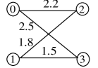
(a) A Gaussian network.

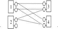
(b) Linear deterministic model.

Figure 1: Linear deterministic model of Gaussian network. (Note $\lfloor\log 2.2^{2}\rfloor=\lfloor\log 2.5^{2}\rfloor=2$, $\lfloor\log 1.8^{2}\rfloor=\lfloor\log 1.5^{2}\rfloor=1$)

The capacity of linear deterministic relay networks with a single source-destination pair is known [2]. Recently the capacity of Gaussian networks with a single source-destination pair was approximately computed [3]. Therefore we can compare them.

II-C Cut-set bound

The cut-set bound [7] of a single source-destination pair network, with source $0$ and destination $M$, is

$$C\ \leq\ \max_{p(x_{0},x_{1},\ldots,x_{M-1})}\ \min_{\Omega\in\Lambda}\ I(X_{\Omega};Y_{\Omega^{c}}|X_{\Omega^{c}}),$$ (1)

where $C$ is capacity of the network $\Lambda$ is the set of all partitions of $\mathcal{V}$ with $0\in\Omega$ and $M\in\Omega^{c}$.

II-C1 Cut-set bounds for linear deterministic networks

Since outputs are a function of inputs in a linear deterministic network, $I(X_{\Omega};Y_{\Omega^{c}}|X_{\Omega^{c}})\ =\ H(Y_{\Omega^{c}}|X_{\Omega^{c}})$. Maximum value of the mutual information equals the rank of the transfer matrix $\mathcal{G}_{\Omega,\Omega^{c}}$ associated with the cut $\Omega$ [2], where the rank is determined over an appropriate finite field. An optimal input distribution is input variables independent and uniformly distributed over the underlying field. Hence (1) simplifies to

$$C\ \leq\ \min_{\Omega}\ \text{rank}\ \mathcal{G}_{\Omega,\Omega^{c}}.$$ (2)

For Fig. 1(b), rank of $\mathcal{G}_{\Omega,\Omega^{c}}$ over $\mathbb{F}_{2}$, with $\Omega=\{0,1\}$, is $2$ with

$$\mathcal{G}_{\Omega,\Omega^{c}}\ =\left[\begin{array}[]{cc}\left[\begin{array}[]{cc}1&0\\ 0&1\end{array}\right]&\left[\begin{array}[]{cc}0&0\\ 1&0\end{array}\right]\\ \left[\begin{array}[]{cc}1&0\\ 0&1\end{array}\right]&\left[\begin{array}[]{cc}0&0\\ 1&0\end{array}\right]\end{array}\right].$$

The cut-set bound in (2) is achieved by random linear coding and hence is the capacity of the network [2].

II-C2 Cut-set bounds for Gaussian Networks

Choosing $\{X_{j}\}$’s to be i.i.d. $\mathcal{CN}(0,1)$ weakens the bound in (1) by at most $(M+1)$ bits for any choice of channel gains and yields

$$\overline{C}\ :=\ \min_{\Omega\in\Lambda}\ \log|I+\mathcal{H}_{\Omega}\mathcal{H}_{\Omega}^{{\dagger}}|,$$ (3)

where $\mathcal{H}_{\Omega}$ is the transfer matrix of the MIMO channel corresponding to cut $\Omega$ and $|.|$ is determinant of the matrix [3].

In [3], a coding scheme is developed that achieves a rate no less than $\overline{C}-\kappa$ for all channel gains, with $\kappa$ only depending on the number $M$ of nodes. Nodes quantize and forward their data and the destination eventually decodes the transmitted symbol after hearing from all the nodes. This scheme is inspired by a coding scheme developed in [2] for a class of general deterministic networks.

III Unbounded capacity difference of linear deterministic model

We will show that capacity of the linear deterministic network can be much lower than that of the original Gaussian network with their difference unbounded as channel gains are varied.

From the previous section, if capacities of the linear deterministic network differed and the Gaussian network differed by a bounded amount, then the difference between their individual cut-set bounds would also be so. We establish unboundedness of the difference by comparing mutual information across cuts in a Gaussian network with ranks of the corresponding cuts in the linear deterministic network.

For the rest we choose the inputs $X_{i}$ for the Gaussian network to be i.i.d. $\mathcal{CN}(0,1)$, noting that this can achieve the maximum mutual information across any cut within a constant bound. For the linear deterministic network, we choose inputs that are independent and uniformly distributed over their range since that maximizes mutual information across a cut.

III-A Counterexample to constant bit approximation

Consider the network in Fig. 2(a) where the channels marked as $\infty$ have very high capacity. The mutual information across $\Omega=\{0,1,2\}$ is

$$I(X_{\Omega};Y_{\Omega^{c}}|X_{\Omega^{c}}) = \log|I+\mathcal{H}\mathcal{H}^{{\dagger}}|$$

$$= 2\log(1+2|h|^{2})$$

$$= 4\log|h|+O(1),\ \text{as }|h|\rightarrow\infty,$$

with $\mathcal{H}\ =\ \left[\begin{array}[]{cc}h&-h\\ h&h\end{array}\right].$ This is the minimum among all cuts and is therefore the capacity.

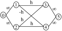
(a) Gaussian network.

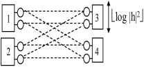
(b) Portion of deterministic network.

Figure 2: Counterexample.

In the corresponding linear deterministic network, the transfer matrix of $\Omega\ =\ \{0,1,2\}$ in Fig. 2(b) is $\mathcal{G}\ =\ \left[\begin{array}[]{cc}I&I\\ I&I\end{array}\right]$, where each identity matrix has dimension $\lfloor\log|h|^{2}\rfloor$. The capacity of the network is the rank of $\mathcal{G}$, i.e., $\lfloor 2\log|h|\rfloor$.

The gap between capacities of the Gaussian network in Fig. 2(a) and its deterministic counterpart is $2\log|h|+O(1)$. Therefore the gap cannot be bounded independently of channel gains.

The linear deterministic model considers only the magnitude of a channel gain and fails to capture its phase. Constructing the deterministic model over a larger prime field does not help either.

III-B Gaussian networks with positive channel gains

Unfortunately phase is not the only problem. We construct a Gaussian network with positive channel coefficients that cannot be approximated by a linear deterministic network.

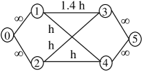
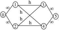
Figure 3: Two networks with positive channel coefficients. Both have the same linear deterministic network in Fig. 2(b) as their counterpart.

Consider the Gaussian networks in Fig. 3, where $h=2^{k}$ for $k\in\mathbb{Z}_{+}$. The linear deterministic network corresponding to both Gaussian networks is the same. However, the difference in the capacities of the Gaussian networks is unbounded.

The capacity of the network in Fig. 3 is

$$C = I(X_{\Omega};Y_{\Omega}^{c}|X_{\Omega}^{c})+O(1)$$

$$= 4\log h+O(1)\ \ (\text{as}\ h\rightarrow\infty),$$

with $\Omega=\{0,1,2\}$, while the capacity of the network in Fig. 3 is

$$\hat{C} = I(X_{\Omega};Y_{\Omega}^{c}|X_{\Omega}^{c})+O(1)$$

$$= 2\log h+O(1)\ \ (\text{as}\ h\rightarrow\infty).$$

So difference in capacities of the linear deterministic network in Fig. 2(b) and at least one of its counterparts in Fig. 3 must be unbounded in $h$.

One may wonder if taking the channel gains into account and quantizing the gains with respect to a field larger than $\mathbb{F}_{2}$ will provide a bounded error approximation. However this reasoning is flawed since then the gap in the capacities would be a function of the chosen prime and thus, in turn, a function of channel gains.

IV Approximating Gaussian networks by discrete superposition networks

A question arises if there is any other deterministic model for approximating Gaussian networks. We now show that an alternate deterministic model, first mentioned in [5], is indeed a good approximation of a Gaussian relay network. This model, which we call a discrete superposition model, captures the phases of channel gains, and ensures that the signal strength does not drop due to quantization of channel gains.

IV-A The discrete superposition model

We define the inputs, outputs, and channels in a discrete superposition network. Let

$$n\ :=\ \max_{(i,j)\in\mathcal{E}}\max\{\lfloor\log|h_{ijR}|\rfloor,\lfloor\log|h_{ijI}|\rfloor\},$$

where $h_{ij}=h_{ijR}+\imath h_{ijI}$. The inputs are complex valued and both real and imaginary parts can take $2^{n}$ equally spaced discrete values from $\{0,2^{-n},\ldots,1-2^{-n}\}$. It helps to think of either the real or imaginary part of an input in terms of its binary representation, i.e., $(x=0.x(1)x(2)\dots x(n))$ with each $x(i)\in\mathbb{F}_{2}$.

The real and imaginary parts of channel gains are quantized to integers by neglecting their fractional parts. The channel between two nodes multiplies the complex input by the corresponding channel gain, and then truncates it by neglecting the fractional components of both real and imaginary parts of the product. The outputs of all incoming channels at a receiver node are complex numbers with integer real and imaginary parts. All the outputs are added up at a receiver by standard summation over $\mathbb{Z}+\imath\mathbb{Z}$.

This model retains the essential superposition property of the channel. The truncation of channel coefficients does not substantially change the channel matrix in the high SNR limit. Also, the effect of noise is captured in essentially the same way as in the linear deterministic model by truncating least significant bits.

This discrete superposition model was first used in [5] in a sequence of networks that reduced the Gaussian interference channel to a linear deterministic network. We use some of the techniques from [5] in the proof below. In [2], it was shown that the cut-set bound is achievable for such deterministic networks, provided attention is restricted to product distributions for the input signals. The main result presented below entails showing that the loss in restricting attention to product distributions for inputs is bounded for discrete superposition relay networks. The connection with Gaussian relay networks or with MIMO channels (see the following Sec. V) was not made in [5]. There is also no cooperation among the input or output nodes in [5], which is a key ingredient of the proof below.

Theorem IV.1

The difference in capacities of a Gaussian relay network with a single source-destination pair and the corresponding discrete superposition network is bounded with the bound depending only on the number of nodes.

Proof:

We prove the result by assuming that the network permits only real valued signals. Extending the result to Gaussian networks with complex valued signals is straightforward, but involves more bookkeeping as noted at the end.

We show that achievable rates in the Gaussian network are within a bounded gap of achievable rates in the discrete superposition network and vice versa.

First we start with the Gaussian network and reduce it to a discrete superposition network in stages, bounding the loss in mutual information at each stage. For specificity consider a cut with two input nodes and two output nodes. Let the output signals be

$$y_{i}=h_{i1}x_{1}+h_{i2}x_{2}+z_{i},\ i=1,2.$$ (4)

Choose $x_{1}$, $x_{2}$ as i.i.d. $\mathcal{N}(0,1)$ (since this choice is approximately optimal in the sense that it maximizes mutual information of the cut up to a constant, see Sec. II-C2). The mutual information across this cut is

$$I(X_{1},X_{2};Y_{1},Y_{2})\ =\ \frac{1}{2}\,\log|I+\mathcal{H}\mathcal{H}^{t}|,$$ (5)

where $\mathcal{H}$ is the channel transfer matrix. Our goal is to derive inputs to the corresponding discrete superposition channel from $x_{1}$ and $x_{2}$ such that mutual information of the deterministic channel differs by no more than a constant from (5).

We begin by scaling all channel gains by half:

$$y_{i}^{{}^{\prime}} := (h_{i1}/2)x_{1}+(h_{i2}/2)x_{2}+z_{i}$$ (6)

$$= h_{i1}^{{}^{\prime}}x_{1}+h_{i2}^{{}^{\prime}}x_{2}+z_{i},\ i=1,2,$$

with $h_{ij}^{{}^{\prime}}:=h_{ij}/2$. The mutual information decreases by at most $1$ bit in comparison to (5), since

$$(I+\mathcal{H}\mathcal{H}^{t})\ \preceq\ 4(I+\frac{\mathcal{H}}{2}\frac{\mathcal{H}^{t}}{2})$$

as positive definite matrices. So,

$$I(X_{1},X_{2};Y_{1},Y_{2})\ \leq\ I(X_{1},X_{2};Y_{1}^{{}^{\prime}},Y_{2}^{{}^{\prime}})+1.$$

Each $x_{i}$ can be split into its integer part $\hat{x}_{i}$ and fractional part $\hat{x}_{i}$. More precisely $\hat{x}_{i}:=(\text{sign }x_{i}))\lfloor|x_{i}|\rfloor$, $\bar{x}_{i}:=x_{i}-\hat{x}_{i}$. We discard $\hat{x}_{i}$ and retain $\bar{x}_{i}$. Since $x_{i}$ satisfies unit average power constraint, $\bar{x}_{i}$ satisfies unit peak power constraint. Define

$$\bar{y}_{i}\ :=\ h_{i1}^{{}^{\prime}}\bar{x}_{1}+h_{i2}^{{}^{\prime}}\bar{x}_{2}+z_{i},\ i=1,2.$$ (7)

Denote the discarded portion of the received signal by

$$\hat{y}_{i}=h_{i1}^{{}^{\prime}}\hat{x}_{1}+h_{i2}^{{}^{\prime}}\hat{x}_{2},\ i=1,2.$$ (8)

Comparing with the channel in (6), we get

$$I(X_{1},X_{2};Y_{1}^{{}^{\prime}},Y_{2}^{{}^{\prime}})$$ (9)

$$\leq I(X_{1},X_{2};Y_{1}^{{}^{\prime}},Y_{2}^{{}^{\prime}},\hat{Y}_{1},\hat{Y}_{2},\bar{Y}_{1},\bar{Y}_{2})$$

$$= I(X_{1},X_{2};\hat{Y}_{1},\hat{Y}_{2},\bar{Y}_{1},\bar{Y}_{2})$$

$$= h(\bar{Y}_{1},\bar{Y}_{2},\hat{Y}_{1},\hat{Y}_{2})-h(Z_{1},Z_{2})$$

$$\leq h(\bar{Y}_{1},\bar{Y}_{2})-h(Z_{1},Z_{2})+H(\hat{Y}_{1},\hat{Y}_{2})$$

$$= I(\bar{X}_{1},\bar{X}_{2};\bar{Y}_{1},\bar{Y}_{2})+H(\hat{Y}_{1},\hat{Y}_{2})$$

$$\leq I(\bar{X}_{1},\bar{X}_{2};\bar{Y}_{1},\bar{Y}_{2})+H(\hat{X}_{1})+H(\hat{X}_{2}),$$

where (9) holds because $\hat{Y}_{i}$’s are a function of $\hat{X}_{i}$’s from (8). Since $X_{i}$ is $\mathcal{N}(0,1)$, we can show that

$$H(\hat{X}_{i})\ =\ -\sum_{k\in\mathbb{Z}}p_{\hat{X}_{i}}(k)\log p_{\hat{X}_{i}}(k)<\ 4.$$

From (9) and above, channel (7) loses at most $8$ bits compared to channel (6).

Since $\hat{x}_{i}$ are not necessarily positive, we obtain positive inputs by adding $(h_{i1}^{{}^{\prime}}+h_{i2}^{{}^{\prime}})$ to $\bar{y}_{i}$:

$$\tilde{y}_{i} := \bar{y}_{i}+h_{i1}^{{}^{\prime}}+h_{i2}^{{}^{\prime}}$$ (10)

$$= h_{i1}(\bar{x}_{1}+1)/2+h_{i2}(\bar{x}_{2}+1)/2+z_{i}$$

$$=: h_{i1}\tilde{x}_{1}+h_{i2}\tilde{x}_{2}+z_{i},\ i=1,2,$$

where now $\tilde{x}_{i}$ lies in $[0,1)$. $I(\tilde{X}_{1},\tilde{X}_{2};\tilde{Y}_{1},\tilde{Y}_{2})$ remains equal to $I(\bar{X}_{1},\bar{X}_{2};\bar{Y}_{1},\bar{Y}_{2})$.

The features of the model that we next address are

1. channel gains are integers,

2. inputs are restricted to
   $n\ :=\ \max_{(i,j)\in\mathcal{E}}\lfloor\log h_{ij}\rfloor$ bits,

3. there is no AWGN, and

4. outputs involve truncation to integers.

Let the binary expansion of $\tilde{x}_{i}$ be $0.\tilde{x}_{i}(1)\tilde{x}_{i}(2)\ldots$. We get the output of the discrete superposition channel by retaining the relevant portion of signal (10):

$$y^{\text{det}}_{i} =: \left\lfloor\hat{h}_{i1}x^{\text{det}}_{1}\right\rfloor+\left\lfloor\hat{h}_{i2}x^{\text{det}}_{2}\right\rfloor,$$ (11)

where $x^{\text{det}}_{i}:=\sum_{k=1}^{n}\tilde{x}_{i}(k)2^{-k}$, and we have truncated channel gains, i.e., $\hat{h}_{ij}:=(\text{sign }h_{ij})\lfloor|h_{ij}|\rfloor$. To get (11) from (10), we subtracted

$$\epsilon_{i} := \sum_{j=1}^{2}\left(h_{ij}(\tilde{x}_{j}-x^{\text{det}}_{j})+(h_{ij}-\hat{h}_{ij})\,x^{\text{det}}_{j}\right.$$ (12)

$$\left.+\ \text{frac}\left(\hat{h}_{ij}\,x^{\text{det}}_{j}\right)\right)+z_{i}$$

$$=: \sum_{j=1}^{2}w_{ji}+z_{i}.$$ (13)

To bound the loss in mutual information, note

$$I(\tilde{X}_{1},\tilde{X}_{2};\tilde{Y}_{1},\tilde{Y}_{2})$$

$$= h(\tilde{Y}_{1},\tilde{Y}_{2})-h(\tilde{Y}_{1},\tilde{Y}_{2}|\tilde{X}_{1},\tilde{X}_{2})$$

$$= h(\tilde{Y}_{1},\tilde{Y}_{2})-h(Z_{1})-h(Z_{2})$$

$$\leq h(Y^{\text{det}}_{1},Y^{\text{det}}_{2},\epsilon_{1},\epsilon_{2})-h(Z_{1})-h(Z_{2})$$

$$\leq H(Y^{\text{det}}_{1},Y^{\text{det}}_{2})+h(\epsilon_{1})+h(\epsilon_{2})$$

$$-\ h(Z_{1})-h(Z_{2}).$$

From the definition of $\epsilon_{i}$ in (12), and since $y^{\text{det}}_{i}$ are completely determined by $x^{\text{det}}_{1},x^{\text{det}}_{2}$, we can rewrite

$$I(\tilde{X}_{1},\tilde{X}_{2};\tilde{Y}_{1},\tilde{Y}_{2})\ \leq\ I(X^{\text{det}}_{1},X^{\text{det}}_{2};Y^{\text{det}}_{1},Y^{\text{det}}_{2})$$

$$+\sum_{i=1}^{2}(h(\epsilon_{i})-h(\epsilon_{i}|W_{1i},W_{2i}))$$

$$\ =\ I(X^{\text{det}}_{1},X^{\text{det}}_{2};Y^{\text{det}}_{1},Y^{\text{det}}_{2})$$

$$+\ I(W_{11},W_{21};\epsilon_{1})+I(W_{12},W_{22};\epsilon_{2}).$$

By bounding the magnitudes of terms in (12), we get $|w_{ji}|\ \leq\ 4$. So, $I(W_{11},W_{2i};\epsilon_{1})$ is the mutual information of a MISO channel with input power constraint $(16+16)=32$ and $I(W_{11},W_{21};\epsilon_{1})\leq\frac{1}{2}\log(1+32)<3$ bits. So we lose at most $6$ bits in the last step.

We have proved that difference between the maximum mutual information across a cut in a Gaussian network and an achievable mutual information for the same cut in the discrete superposition network is bounded. Repeating this for every cut yields a bound that depends solely on number of nodes.

Conversely, start with a joint distribution for inputs $x^{\text{det}}_{i}$ in the discrete superposition network. Since $x^{\text{det}}_{i}$’s satisfy average power constraint, we can apply them directly to the Gaussian channel to get

$$y_{i}\ =\ h_{i1}x^{\text{det}}_{1}+h_{i2}x^{\text{det}}_{2}+z_{i},i=1,2.$$

We can rewrite $y_{i}$ as

$${y_{i}} = y^{\text{det}}_{i}+\sum_{j=1}^{2}\left((h_{ij}-\hat{h}_{ij})\,x^{\text{det}}_{j}\right.$$

$$\left.+\ \text{frac}(\hat{h}_{ij}\ x^{\text{det}}_{j})\right)+z_{i}$$

$$=: y^{\text{det}}_{i}+\sum_{j=1}^{2}v_{ji}+z_{i},\ i=1,2.$$

By definition $y^{\text{det}}_{i}$ takes on only integer values. Hence $y^{\text{det}}_{i}$ can be recovered from $y_{i}$, the integer parts of $v_{ji}$’s and noise $z_{i}$, and the carry $c_{i}$ obtained from adding the fractional parts of $v_{ji}$’s and $z_{i}$. So,

$$I(X^{\text{det}}_{1},X^{\text{det}}_{2};Y^{\text{det}}_{1},Y^{\text{det}}_{2})$$

$$\leq I(X^{\text{det}}_{1},X^{\text{det}}_{2};Y_{1},Y_{2},\{\hat{V}_{ji}\},\{\hat{Z}_{i}\},\{C_{i}\})$$

$$\leq I(X^{\text{det}}_{1},X^{\text{det}}_{2};Y_{1},Y_{2})+\sum_{i,j=1}^{2}H(\hat{V}_{ji})$$

$$+\sum_{i=1}^{2}H(\hat{Z}_{i})+\sum_{i=1}^{2}H(C_{i}).$$

Here $\hat{v}_{ji}$, $\hat{z}_{i}$ are integer parts of the respective variables. Since $|v_{ji}|\leq 2$, $\hat{v}_{ji}\in\{-2,-1,\ldots,2\}$, and $H(\hat{V}_{ji})\leq 3$. The carry $c_{i}\in\{-2,-1,\ldots,2\}$, hence $H(C_{i})\leq 3$. As earlier, $H(\hat{Z}_{i})\leq 4$. Therefore mutual information of the Gaussian channel is at most $28$ bits lesser than that of the discrete superposition channel.

Above arguments can be extended to show that for every joint distribution for inputs in the discrete superposition channel, there is a product distribution for inputs with a bounded reduction in the mutual information. To complete the proof we note that the cut-set bound in (1) restricted to product distributions is achievable in the discrete superposition network [2].

For the general case of complex Gaussian networks, we allow signals in (4) to be complex valued and rewrite

$$\left[\begin{array}[]{c}y_{iR}\\ y_{iI}\end{array}\right]\ =\ \left[\begin{array}[]{cc}h_{i1R}&-h_{i1I}\\ h_{i1I}&h_{i1R}\end{array}\right]\left[\begin{array}[]{c}x_{1R}\\ x_{1I}\end{array}\right]$$

$$+\left[\begin{array}[]{cc}h_{i2R}&-h_{i2I}\\ h_{i2I}&h_{i2R}\end{array}\right]\left[\begin{array}[]{c}x_{2R}\\ x_{2I}\end{array}\right]+\left[\begin{array}[]{c}z_{R}\\ z_{I}\end{array}\right].$$

Now choose inputs to be i.i.d. $\mathcal{CN}(0,1)$. Increasing variances of both inputs and Gaussian noise from $1$ to $2$ does not change the mutual information, though now $X_{iR}$, $X_{iI}$, $Z_{R}$, $Z_{I}$ are $\mathcal{N}(0,1)$. Rest of the analysis can be repeated. ∎

V MIMO channels and deterministic models

Above we analyzed a network by comparing the MIMO channels corresponding to the same cut in the Gaussian network and its deterministic counterpart. We can easily extend the negative result in Sec. III to show that, in general, MIMO channels cannot be approximated by the linear deterministic model. In the same vein, we can extend the positive result in Sec. IV to prove that the discrete superposition model remains a good approximation for MIMO Gaussian channels.

VI Concluding remarks

Since the capacity of the linear deterministic model does not approximate that of the Gaussian relay network, the challenge is to quantitatively show to what extent, how, and why good coding strategies for the former yield good strategies for the latter.

For discrete superposition networks, the challenge is to extend the bounded error approximation result to networks with multiple sources and destinations.

References

- [1] A. S. Avestimehr, S. N. Diggavi, and D. N. C. Tse, “A Deterministic Approach to Wireless Relay Networks,” Proc. 45th Annu. Allerton Conf., Monticello, IL, Sept. 2007.
- [2] ———–, “Wireless Network Information Flow,” Proc. 45th Annu. Allerton Conf., Monticello, IL, Sept. 2007.
- [3] ———–, “Approximate Capacity of Gaussian Relay Networks,” Proc. of IEEE ISIT 2008, Toronto, Canada, July 2008.
- [4] A. S. Avestimehr, A. Sezgin, and D. N. C. Tse, “Approximate capacity of the two-way relay channel: A deterministic approach,” Proc. 46th Annu. Allerton Conf., Monticello, IL, Sep. 2008.
- [5] G. Bresler and D. N. C. Tse, “The two-user Gaussian interference channel: a deterministic view,” arXiv:0807.3222v1
- [6] V. R. Cadambe, S. A. Jafar, and S. Shamai, “Interference Alignment on the Deterministic Channel and Application to Fully Connected AWGN Interference Networks,” accepted for publication in the IEEE Trans. on Info. Theory. arXiv: 0711.2547.
- [7] A. El Gamal, “On Information Flow in Relay Networks,” IEEE National Telecomm. Conf., Vol. 2, pp. D4.1.1 - D4.1.4, Nov. 1981.
- [8] R. Etkin, D. N. C. Tse, and H. Wang, “Gaussian Interference Channel Capacity to Within One Bit,” arXiv: 0702045v2.
- [9] A. S. Avestimehr, “Wireless network information flow: a deterministic approach,” Ph.D. dissertation, Univ of California, Berkeley, Oct. 2008.