Individual and Group Galaxies in CNOC1 Clusters

Abstract

Using wide-field $BVR_{c}I$ imaging for a sample of 16 intermediate redshift ($0.17<z<0.55$) galaxy clusters from the Canadian Network for Observational Cosmology (CNOC1) Survey, we investigate the dependence of cluster galaxy populations and their evolution on environment. Galaxy photometric redshifts are estimated using an empirical photometric redshift technique and galaxy groups are identified using a modified friends-of-friends algorithm in photometric redshift space. We utilize the red galaxy fraction ($f_{red}$) to infer the evolutionary status of galaxies in clusters, using both individual galaxies and galaxies in groups. We apply the local galaxy density, $\Sigma_{5}$, derived using the fifth nearest-neighbor distance, as a measure of local environment, and the cluster-centric radius, $r_{CL}$, as a proxy for global cluster environment. Our cluster sample exhibits a Butcher-Oemler effect in both luminosity-selected and stellar-mass-selected samples. We find that $f_{red}$ depends strongly on $\Sigma_{5}$ and $r_{CL}$, and the Butcher-Oemler effect is observed in all $\Sigma_{5}$ and $r_{CL}$ bins. However, when the cluster galaxies are separated into $r_{CL}$ bins, or into group and non-group subsamples, the dependence on local galaxy density becomes much weaker. This suggests that the properties of the dark matter halo in which the galaxy resides have a dominant effect on its galaxy population and evolutionary history. We find that our data are consistent with the scenario that cluster galaxies situated in successively richer groups (i.e., more massive dark matter halos) reach a high $f_{red}$ value at earlier redshifts. Associated with this, we observe a clear signature of ‘pre-processing’, in which cluster galaxies belonging to moderately massive infalling galaxy groups show a much stronger evolution in $f_{red}$ than those classified as non-group galaxies, especially at the outskirts of the cluster. This result suggests that galaxies in groups infalling into clusters are significant contributors to the Butcher-Oemler effect.

1 Introduction

With increasingly detailed studies of galaxy properties such as stellar population and morphology, our knowledge of galaxies in the Universe has greatly improved. The large-scale structure in the Universe shows that some galaxies are located in low-density filaments while others populate high-density clusters. This complicates our understanding of galaxy evolution over the Hubble time, because galaxy properties depend not only on time but also on environment. Therefore, in order to understand galaxy evolution in the Universe, galaxy properties require viewing simultaneously and systematically over time and in different environments.

The morphology-density relation (Dressler, 1980) is well-accepted evidence for the environmental dependence of galaxy properties. Early-type galaxies favor dense environments, while late-type galaxies are common in less dense environments. Following this pioneering work, a considerable number of studies on this topic have been carried out or extended (e.g., Domínguez et al., 2002; Goto et al., 2003; Hogg et al., 2003; Tanaka et al., 2005; Nuijten et al., 2005), showing that environment is an important predictor of galaxy properties.

Abundant in galaxy aggregations, clusters of galaxies offer the best sites to study such environmental effects. The observation that clusters at higher redshift contain a larger portion of blue galaxies is commonly referred to as the Butcher-Oemler effect (e.g., Butcher & Oemler, 1984; Poggianti et al., 2006; Ellingson et al., 2001; Gerke et al., 2007). The increase by $\sim 20\%$ in the blue galaxy fraction from $z$=0.03 to $z$=0.50 in the Butcher-Oemler effect suggests that star forming activity in galaxy clusters decreases toward the nearby Universe. With the continuous accretion of field galaxies into galaxy clusters, this decrease implies that star formation is inhibited by the cluster environment.

However, the fraction of galaxies located in these densest galaxy environments is only $\sim 10\%$ even at the present epoch. Groups of galaxies, the intermediate density locations between dense clusters and the sparse field, are the most common environment where galaxies are found. Seeded by lower-density perturbations in a hierarchical Universe, galaxy groups have a large variety of galaxy densities, from early-collapsed ‘fossil groups’ to aggregations of a few galaxies with densities only slightly greater than that of the field. With relatively small velocity dispersions compared with clusters, galaxy groups are also the favored environment for slow dynamical encounters, leading to mergers (e.g., Mamon, 2000; Coziol & Plauchu-Frayn, 2007). Furthermore, a higher fraction of passive galaxies have been observed in galaxy groups than in the field (e.g., Wilman et al., 2005, 2008; Yan et al., 2008). A sort of morphology segregation in galaxy groups is observed in the nearby Universe, as early-type galaxies are more commonly located in the group centers and spirals have larger projected centric distance from the host groups (e.g., Jeltema et al., 2007; Verdugo et al., 2008). The underlying mechanisms which drive a similar trend in the morphology-density relation in clusters may also exist in galaxy groups (e.g., Helsdon & Ponman, 2003a, b; Mulchaey & Zabludoff, 1998).

A wide variety of observations in both optical and X-ray regimes has provided convincing evidence that substructures in clusters are common. Rich galaxy clusters are believed to be built up by infalling galaxy groups (e.g., Bekki, 1999; Solanes et al., 1999; Abraham et al., 1996; Adami et al., 2005; Krick et al., 2006), while galaxies in a group may have evolved already before the whole group falls into a cluster: i.e., what is referred to as pre-processing (Fujita, 2004). However, there is still considerable uncertainty on the roles that these smaller structures play in the star formation history of cluster galaxies. Therefore, cluster and group galaxy populations give us a unique opportunity to study the environmental effect on large (global, or ‘cluster’) and small (local, or ‘group’) scales.

In order to unfold the role of time and environment in galaxy evolution in clusters, we study these two major factors using both individual galaxies and galaxy groups in 16 clusters from the Canadian Network for Observational Cosmology (CNOC1) multi-band $BVR_{c}I$ photometric observations. The structure of this paper is as follows. We present the data in $\S$2. We then briefly describe the photometric redshift method and sample selection in $\S$3. The group finding method is briefly presented in $\S$4. The identification of cluster galaxies and groups is detailed in $\S$5. We present the calculations of the environmental parameters and red galaxy fraction in $\S$6. We describe the correction due to background contamination in $\S$7. We present the results $\S$8 and discuss their implications in $\S$9. Finally a summary is presented in $\S$10. We adopt $\Omega_{m}$=0.7, $\Omega_{\Lambda}$=0.3, and $H_{0}$=70 km/s/Mpc.

2 The Cluster Catalogs

2.1 The Data

The original CNOC1 Cluster Redshift Survey (Yee et al., 1996) contains 16 rich X-ray selected galaxy clusters at $0.17<z<0.55$, and was carried out with the main goal of measuring the cosmological density parameter, $\Omega_{m}$. The observations were made using the CFHT Multi-Object-Spectrograph (MOS) with Gunn $g$ and $r$ images to $r\sim 24$ and spectroscopy to $r\sim 21.5$. The multi-color photometric follow-up observations in this study targeted 15 of the CNOC1 clusters using the CFHT 12K camera in 2000 and 2001. The camera, composed of 12 chips of 2045 $\times$ 4096 pixels with 0.206$\arcsec$ per pixel, has a $42\arcmin\times 28\arcmin$ field of view. Ten clusters were taken from classical observations and the other five were from queue observations. Among these 15 clusters, 14 were observed using $BVR_{c}I$ filters with seeing ranging from $\sim 0.70\arcsec$ to 1.24″ in the $R_{c}$-passband. MS0015+16 (CL0015+16, $z$=0.55) was observed in $B$ and $V$ only, and hence is excluded for not having enough passbands for our photometric redshift method. We also exclude the MS1224+20 field because the observations were non-photometric and not sufficiently deep for our scientific goals. MS1006+12 was omitted due to a very bright star in the field. MS0302+16 ($z$=0.425, $\alpha_{2000}$=03:05:35.42, $\delta_{2000}$=17:10:3.43) was targeted incorrectly to MS0302.5+1717 ($z$=0.425, $\alpha_{2000}$=03:05:18.110, $\delta_{2000}$= 17:28:24.92), about 18.82′ north from the original CNOC1 target. Another cluster, CL0303+1706 (z=0.418, $\alpha_{2000}$=03:06:18.7, $\delta_{2000}$= +17:18:03), is in the south-east of MS0302.5+1717.

The pointings for MS1231+15 and MS1358+62 contain other clusters in the field. Abell 1560 ($\alpha_{2000}$=12:34:07.1, $\delta_{2000}$=15:10:28, $z$=0.244; Abell et al., 1989; Ulmer & Cruddace, 1982; David et al., 1999) is south of MS1231+15. MS1358+62 has been known as a binary cluster in the CNOC1 analysis (Carlberg et al., 1996). The other cluster in the MS1358+62 field is at $\alpha_{2000}$=13:59:39.511, $\delta_{2000}$=62:18:47.0, with $z$=0.329. In summary, our data set contains 12 CNOC1 clusters and 4 other confirmed clusters. The sample properties and exposure times are listed in Tables 1 and 2.

2.2 Photometry and Color Calibration

For the queue-observed data, the basic data reduction and calibration steps were undertaken using the Elixir system at CFHT . For the classically observed data, the data reduction proceeded in the standard way using IRAF (http://iraf.noao.edu/) including bias subtraction and flat fielding. The photometric calibration was performed using images of standard star fields from Landolt (1992).

The object finding, aperture photometry, and star-galaxy classification were carried out using the Picture Processing Package (PPP), details of which are described in Yee (1991) and Yee et al. (1996). Here we present a brief summary of the procedures. This algorithm detects objects by the locations of brightness peaks above a preset threshold level and satisfying a number of criteria (e.g., a minimum number of connected pixels, a sharpness test, etc., see Yee et al. 1996). In general, about 2,000 to 3,000 objects on average were detected in each chip. The photometry is achieved by constructing and analyzing the flux growth curve of an object. The total magnitude is measured in an ‘optimal aperture’, and then corrected to a standard aperture of $8.5\arcsec$ diameter using the PSF profile of reference stars, if the optimal aperture of the object is smaller than the standard aperture. The color of each object is measured independently from the total magnitude, using a ‘color aperture’ of $3\arcsec$, or the optimal aperture, whichever is smaller. The total magnitude for the second filter is then computed from the color and the total magnitude of the first filter. The star-galaxy classification is accomplished by comparing the growth curve of each object to a local set of bright, but not saturated, reference stars. The algorithm classifies objects into four categories: galaxies, stars, saturated stars, and spurious ‘non-object’ (e.g., cosmic ray detections or cosmetic defects).

In order to check the photometry of the CNOC1 follow-up observations, we compare our $R_{c}$ data with the Gunn $r$ photometry obtained by the original CNOC1 program, using the transformation $r=R_{c}+0.28+0.027\times(B-R_{c})$ derived from stars in the M67 field. To check the color offsets in the other passbands, we use the calibrated $R_{c}$ photometry as the reference. For $B$ and $V$ photometry, we compare the star colors with those in the Red-Sequence Cluster Survey (RCS; Gladders & Yee, 2005) CFHT patches (Hsieh et al., 2005) using bright stars ($18\leq R_{c}\leq 22$). Because the RCS uses $BVR_{c}z^{\prime}$ instead of $BVR_{c}I$ passbands, we compare the distributions of $I-R_{c}$ star colors with those in the MS1231+15, MS1455+22, and MS1512+36 fields. These three pointings have been processed using the Elixir system, for which the $I$-band photometry is consistent with each other after being cross-checked. The zero points in $BVI$ are shifted if any color offsets are present.

2.3 Astrometry

Astrometry for each frame is calibrated using the IRAF package MSCRED with USNO-a2 catalogs. The MSCRED package has the ability to operate on multi-chip CCD data simultaneously without the need to split each image frame into separate CCD images and process them individually. Therefore, each CNOC1 12K follow-up observation pointing is made into a multi-extension FITS with 12 extensions. An astrometry calibration file is generated by the msctpeak command based on the MS0302+16 field. After updating the image headers with the calibration file, the mscczero and msccmatch commands are used to apply the shifts and match the positions between the objects on the images and in the USNO-a2 catalogs. We also update the astrometry in the headers of the original CNOC1 MOS images, so the object list from the CFH-12K data can be easily matched with those spectroscopically observed using MOS.

3 Photometric Redshift and Sample Selection

The photometric redshift technique allows us to estimate galaxy redshifts using photometry information. Because the information obtained from photometric redshifts is less accurate, the use of the technique requires careful consideration in selecting the samples. In this section we present briefly the photometric redshift technique and the sample selection; details can be found in Li & Yee (2008).

3.1 Redshift Estimation

Galaxy redshifts are estimated using an empirical photometric redshift technique from Li & Yee (2008). This technique assumes that redshift is a polynomial function of galaxy colors and magnitudes. The coefficients of this polynomial can be estimated by fitting the galaxies in a training set, which is a catalog containing galaxy spectroscopic redshifts and magnitudes. Our training set contains 3988 galaxies in $BVR_{c}Iz^{\prime}$ up to $z\sim 1.4$ with $R_{c}<24.$, constructed from the Hubble Deep Field (Giavalisco et al., 2004) and CNOC2 catalogs (Yee et al., 2000). The properties of the training set are described in Hsieh et al. (2005) and Li & Yee (2008). To achieve better-constrained solutions, the galaxies with spectroscopic redshifts in the CNOC1 sample (2022 galaxies in total) are added to the training set. The photometric redshift uncertainties and probability densities of individual galaxies, $P(z)$, are obtained as part of our photometric redshift technique as well.

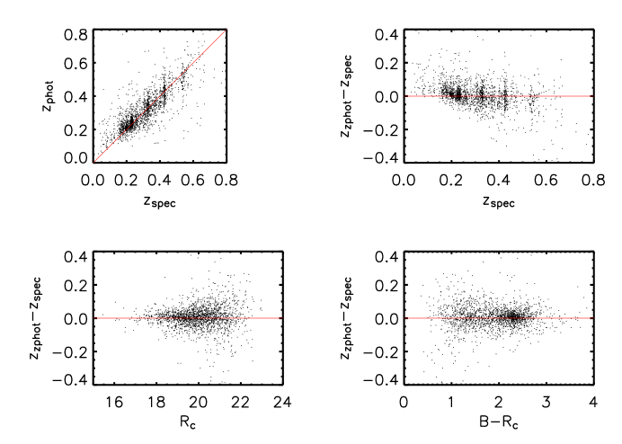
Figure 1: The estimated photometric redshift for 2022 CNOC1 galaxies with spectroscopic redshifts. The top two panels show the comparison between the spectroscopic and photometric redshifts. The overall dispersion is $\sigma(z_{phot}-z_{spec})\sim 0.051$. At $z<0.1$, the photometric redshift measurements are affected by not having a sufficiently blue band. The bottom two panels plot $z_{phot}-z_{spec}$ as functions of galaxy magnitude and color. The scatter is larger toward fainter magnitudes and blue colors: $\sigma(z_{phot}-z_{spec})\sim 0.048$ and $\sim 0.108$ for $R_{c}<21.5$ and $R_{c}\geq 21.5$, respectively, and $\sigma(z_{phot}-z_{spec})\sim 0.041$ for $B-R_{c}\geq 1.8$ and $\sim 0.070$ for $B-R_{c}<1.8$

To assess the accuracy of our photometric redshifts, we compare them with the spectroscopic redshifts of the 2022 CNOC1 galaxies. The differences between photometric and spectroscopic redshifts are plotted in Figure 1 as functions of galaxy magnitude and $B-R_{c}$ color. The overall r.m.s., $\sigma(z_{phot}-z_{spec})$, is $\sim 0.051$, with $\sigma(z_{phot}-z_{spec})\sim 0.048$ and $\sim 0.108$, for $R_{c}<21.5$ and $R_{c}\geq 21.5$, respectively. Blue galaxies (defined by $B-R_{c}<1.8$) has $\sigma(z_{phot}-z_{spec})\sim 0.070$, while $\sigma(z_{phot}-z_{spec})$ is $\sim 0.041$ for red galaxies (defined by $B-R_{c}\geq 1.8$).

3.2 Galaxy Sample Selection

For our analysis, we construct a sample of galaxies with a photometric redshift range of $0.02\leq z\leq 1.4$. The upper photometric redshift limit is due to the passband wavelength coverage for the $4000$ Å break in our training set. We select galaxies by their photometric redshift probability densities. The photometric redshift probability densities used are consistent with the observed scatter in $z_{phot}-z_{spec}$ in the training set for different types of galaxies. The selection criterion for galaxy $i$ is set as:

$$\int_{z_{i}-3\sigma_{z}}^{z_{i}+3\sigma_{z}}P_{i}(z^{\prime})dz^{\prime}>0.997,$$ (1)

with $\sigma_{z}$ set to 0.2(1+$z$), which is equivalent to excluding galaxies whose photometric redshift uncertainty is greater than 0.2(1+$z$).

Each galaxy in the sample is then assigned a completeness correction weight, $w_{i}$, to account for galaxies excluded from the sample due to the $\sigma_{z}$ criterion. The completeness correction is computed using the ratio of the total number of galaxies to the number of galaxies satisfying our selection criteria in magnitude bins of $\Delta m_{R_{c}}=0.1$. We set a cutoff in $R_{c}$ based on where $w_{i}=2$ to avoid high weight galaxies. This apparent magnitude cutoff is brighter than the 100% photometric completeness magnitude in all cases, and ranges from 22.12 to 22.80 for the different pointings. The median and mean of the completeness correction factor $w_{i}$ in the sample are $\sim 1.08$ and $\sim 1.20$, respectively.

The sample used for group finding is limited to galaxies with k- and evolution-corrected $R_{c}$-band absolute magnitude, $M_{R_{c}}^{k,e}$, brighter than $M^{*}_{R_{c}}+2$. We adopt $M^{*}_{R_{c}}$=-21.41 at $z=0$ (Kodama & Arimoto, 1997). The k-correction is computed using the tabulated values from Poggianti (1997) for different spectral energy distributions (SED). For each galaxy, we interpolate the k-correction values between the E/S0 and Sc SEDs based on its $B-R_{c}$ color. We note that when selecting galaxies at different redshifts using k-corrections derived from galaxy colors creates a less biased sample than applying k-corrections averaged over SED types without using color information (e.g., see Loh et al., 2008). The $R_{c}$ luminosity evolution is approximated as $M(z)=M(0)-zQ$, where Q=1.24 for red galaxies and Q=0.11 for blue galaxies (Lin et al., 1999). In the cases when the apparent magnitude limit is brighter than $M^{*}_{Rc}+2$ at the photometric redshift of the group, we apply a correction factor $R_{w}$ which is the ratio of the integral of the galaxy luminosity function (LF) integrated to $M^{*}_{Rc}+2$ to that integrated to the completeness limit (see Eqn 2 in Li & Yee 2008), to correct for the expected missing galaxy counts in these fields. Note that while we use $M^{*}_{R_{c}}+2.0$ as the limit of pFoF group finding (which optimizes group-finding results), we limit the galaxy sample to $M^{*}_{R_{c}}+1.5$ for our galaxy population analysis.

4 Identifying Galaxy Groups

Galaxy groups in the photometric redshift catalogs are identified using the ‘Probability Friends-of-Friends’ algorithm (pFoF); a modified friends-of-friends group-finding algorithm which takes into consideration the photometric redshift probability density of each galaxy and group. Detailed descriptions of the algorithm and performance tests are presented in Li & Yee (2008); we provide a brief summary below. The main idea behind this algorithm is to treat the common photometric redshift space of the transversely connected galaxies as the group redshift space, which changes dynamically as new members are linked in. This updated group redshift is then used to search for more new members. Generally speaking, the group redshift is well confined by the group members, especially when the number of its members is large. The linking criteria are set by two parameters: $D0_{xy}$ and $P_{ratio,crit}$. The $D0_{xy}$ is the reference physical transverse linking length at $z$=0, which is scaled by $(1+z)^{-1}$. In practice, the linking length includes the adjustments for the completeness correction, $w_{i}$, and the varying galaxy numbers at different redshifts due to the apparent magnitude cutoff. $P_{ratio,crit}$ is the criterion used in determining friendship in redshift space, where $P_{ratio}$ denotes the normalized total photometric redshift probability for a galaxy being in the same redshift space as another galaxy or a group of galaxies (see Li & Yee 2008 for details). The parameter $P_{ratio}$ essentially measures the amount of overlap in the photometric redshift probability distributions of the two objects being considered. Galaxies must have $P_{ratio}\geq P_{ratio,crit}$ in order to join into the group. We note that for the purpose of creating the group catalog the algorithm assigns a group membership to every galaxy , with isolated galaxies being identified as groups of one.

This algorithm has been tested using mock catalogs constructed from the Virgo Consortium Millennium Simulation (Springel et al., 2005), including the effects of using different linking criteria. With a fixed $P_{ratio,crit}$, the recovery rate increases when larger $D0_{xy}$ is used; but the use of a larger $D0_{xy}$ also increases the fraction of falsely detected groups. With a given $D0_{xy}$, the recovery rate is better when a smaller $P_{ratio,crit}$ is used, but the false detection rate is larger as well. As a compromise between the recovery and false detection rates, the set of $P_{ratio,crit}=0.37$ and $D0_{xy}=0.25$ Mpc gives the best results. With these parameters, the recovery rate is greater than 80% for mock groups of halo mass $M_{halo}$ greater than $\sim 1.2\times 10^{13}M_{\sun}$, and the false detection rate is less than 10% when a pFoF group contains $\sim 8$ or more net members (corresponding to $M_{halo}\sim 3.7\times 10^{13}M_{\sun}$). The estimated pFoF group redshift uncertainty is $\Delta z_{grp}\sim 0.020$. We adopt $P_{ratio,crit}=0.37$ and $D0_{xy}=0.25$ Mpc for the group-finding procedure in this paper.

For our analysis, we select groups with richness $N_{gal}\geq 8$ and $N_{gz}\geq 7$, where $N_{gal}$ is the net weighted galaxy number, and $N_{gz}$ is the actual number of the linked group members returned by the pFoF algorithm. From the 13 pointings we identify a total of 188 groups satisfying our richness selection using the adopted pFoF parameters, including the cluster cores themselves.

5 The Sample of Cluster Galaxies and Groups

5.1 The Cluster as the Main Group

Generally speaking, galaxy clusters can be treated as exceptionally rich galaxy groups. Because our sample is selected from the follow-up observations of CNOC1 clusters with cluster redshift information available, we identify the galaxy group that coincides with the cluster center position as the main body, or core, of each cluster.

The center of a group is determined using its members in the dense region where their local galaxy densities (see §6.1) are above the mean value of the group members. The center is calculated as the mean R.A. and Dec. of these members, weighted by their luminosity, completeness correction $w_{i}$, and local galaxy density. If a group’s members are distributed in more than one dense region (i.e., clumps in the contours of local galaxy density), only galaxies in the clump which has the largest galaxy number counts are used. To designate the main galaxy aggregation, or the core, of a cluster, each galaxy group is assigned a score based on: (1) the inverse of the separation between the group and cluster centers, (2) the agreement of the group redshift compared with the cluster spectroscopic redshift, and (3) the group richness. The galaxy group which has the best score is chosen as the cluster main-group, i.e., the core galaxy aggregation of a cluster. We emphasize that cluster main-group associated with each galaxy cluster does not contain the whole of the cluster, but rather just the galaxies in the core that satisfy the linking criteria of the pFoF algorithm.

The redshifts of our 16 main cluster galaxy aggregations ($z_{pFoF,cl}$) compared with the spectroscopic redshifts ($z_{spec,cl}$) have a dispersion of $\sigma(z_{pFoF,cl}-z_{spec,cl})\sim 0.019$. The centers of our cluster main-groups are on average $\sim 30\arcsec$ from the physical centers (i.e., where the cD galaxies are). The basic properties of our 16 identified cluster main-groups are listed in Table 3.

5.2 Cluster Galaxies and Groups

To identify galaxies and groups in the cluster redshift space, we follow the same idea used in determining group membership in the pFoF algorithm (Li & Yee 2008), but applied only in the redshift direction without considering the transverse friends-of-friends criterion. That is, the $P_{ratio}$ of each galaxy or group with respect to the redshift probability density of the cluster main-group should satisfy $P_{ratio}\geq P_{ratio,crit}$, with the same $P_{ratio,crit}$ value used in the pFoF algorithm. The galaxies and groups that satisfy this condition are then considered to be in the large scale structure that make up the cluster, including galaxies at large cluster-centric radii.

Applying the pFoF criteria to our group sample with respect to the cluster main-groups, we find 89 groups (not counting the cluster main-groups) consistent with being in the same redshift space as the clusters. Of these, 59 are within 3$R_{200}$ of the cluster centers. Similarly, we apply the pFoF criteria to individual galaxies brighter than $M^{*}_{Rc}+1.5$ to create a sample of galaxies considered to be in the redshift space of the clusters. Hereafter, by ‘cluster galaxies’ or ‘cluster groups’, we mean galaxies or groups whose photometric redshift probability densities within the cluster redshift space satisfy the $P_{ratio,crit}$ criterion. Based on the overall group sample and the typical uncertainty in the photometric redshifts for the groups, we estimate that the cluster group sample may be contaminated by projection (i.e., groups not associated with the same large scale structure in which the the galaxy cluster resides) at a rate of $\sim 0.25$ groups per cluster, sufficiently small that the effect can be ignored in our analysis.

We note that two pointings, 0302+16 and MS0451-03, are not complete to $M^{*}_{Rc}+1.5$ at the cluster redshifts. For these clusters, we apply a correction factor, $R_{w}$ (see §3.2), based on the galaxy LF, to correct the counts to the $M^{*}_{Rc}+1.5$ limit. Note that this correction factor is not strictly correct when used for estimating the red galaxy fraction $f_{red}$ (see §6.3), since the red and blue cluster galaxy LFs are not expected to be identical (e.g., Barkhouse et al., 2007), and will tend to decrease the estimated $f_{red}$ due to the steeper faint end of the blue galaxy LF. However, since our adopted absolute magnitude limit is relatively bright and the incompleteness ranges from 0.05 to 0.3 mag, this effect does not significantly affect our conclusions.

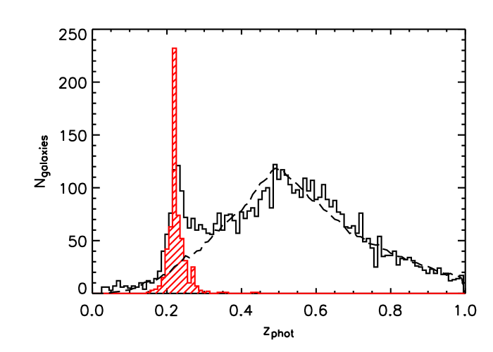
Figure 2: The photometric redshift distribution (open histogram) of all galaxies with $m_{R_{c}}<22.80$ in the field of Abell 2390 field ($z=0.23$). The background galaxy distribution estimated by the RCS CFHT patches (Hsieh et al. 2005) is shown as the dashed line. The cluster galaxies (hatched histogram), as determined by the group finding algorithm (see $\S$4), show a large excess in galaxy number in photometric redshift space at the cluster redshift.

We present an example in Figure 2 using the cluster Abell 2390 ($z=0.228$) to illustrate the selection of cluster galaxies using photometric redshifts. The cluster galaxies, whose memberships are determined using the redshift assigned by the group finding algorithm, exhibit an excess peak in the photometric redshift space in contrast to the field galaxy distribution. Our method of selecting cluster galaxies and groups with reassignment of their redshifts to those of the associated pFoF groups eliminates foreground and background galaxies with higher efficiency than the usual method of applying a photometric redshift cut based on the individual galaxy’s original photometric redshift and uncertainty.

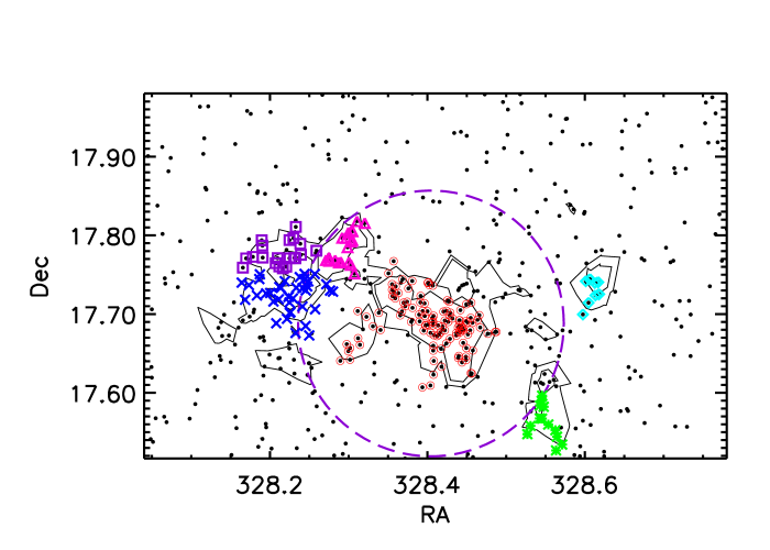
Figure 3: The map of Abell 2390 with groups found using the pFoF algorithm. Galaxies selected in the cluster redshift space are plotted as dots. The symbols with different shapes denote members of cluster groups with $N_{gal}\geq 8$. The cluster main-group members are marked by open circles. The contours of the local projected galaxy density $\Sigma_{5}$, calculated using on all cluster galaxies, are overlaid with levels of $\Sigma_{5}$=20 and 40 gal/Mpc². The dashed circle has a radius of 1 $R_{200}$.

Figure 3 shows the sky locations for the cluster galaxies and cluster groups in the Abell 2390 field. The cluster has an elongation from the central core at about –50⁰ from the N-S axis, spanning both sides of the cD galaxy (Abraham et al., 1996; Pierre et al., 1996). An infalling sub-component at the projected distance of $\sim 650\arcsec$ to the cluster center has been studied in Abraham et al. (1996). This group is identified by the pFoF algorithm as well, and is marked by crosses in Figure 3. Our pFoF algorithm also identifies two additional groups in the same direction, which are marked as squares and triangles in Figure 3. However, as they lie about 100″ and 280″ away from the spectroscopically identified group, these two groups do not contain any members in the original CNOC1 spectroscopic coverage.

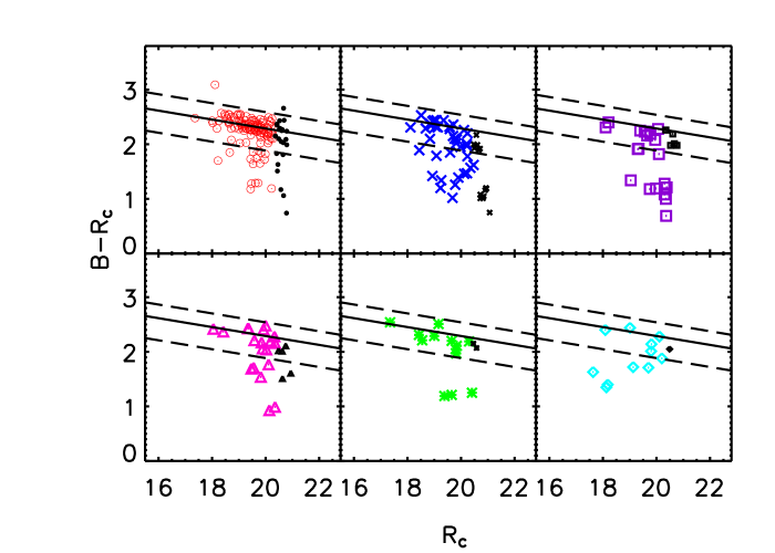
Figure 4: The observed color-magnitude diagram of galaxies ($M_{Rc}^{k,e}<M^{*}_{R_{c}}+2.0$) of galaxies in the cluster main-group and galaxy groups in Abell 2390. The theoretical red-sequence (Kodama & Arimoto, 1997), adjusted for calibration systematics (see §6.3), is overlaid in each panel as the solid line, while the dashed lines define the region used for red galaxies in the calculation of $f_{red}$. Group galaxies in each panel are plotted using the symbol corresponding to the same group in Figure 3. Large symbols mark galaxies with $M_{Rc}^{k,e}<M^{*}_{R_{c}}+1.5$, which are used for the computation of $f_{red}$.

We also present the observed color-magnitude diagrams in Figure 4 for all these cluster groups. Galaxies in the cluster main-group exhibit a well-defined red sequence, while galaxies in the other groups have visually somewhat less prominent red sequences, primarily due to the small number of galaxies. We note that galaxies in groups in clusters may also include some galaxies from the main cluster in projection, which will produce systematically redder groups closer to the cluster core. However, this effect on the average colors of the richer cluster groups used in our analysis (§8.4) is likely to be minimal. The typical galaxy surface density for groups with 8 members or more is 21.56 galaxies/Mpc², whereas the average non-group cluster galaxy surface density at $r_{CL}$=0.5-1.5 ranges from 2.43 to 5.95 galaxies/Mpc², and is as low as 2.05 galaxies/Mpc² at the largest radii we probe.

6 The Environmental Parameters and Red Fraction, $f_{red}$

We intend to study the colors of cluster galaxies in different environments with the aim of identifying environmental effects on galaxy evolution. For this purpose, we demarcate the environmental effect into local and global regimes, and use the fraction of red galaxies as an indicator of their evolutionary stage. Here, we present our methods for computing the environmental parameters and the red galaxy fraction.

6.1 Local Galaxy Environment: Local Galaxy Density $\Sigma_{5}$

For each galaxy, the local galaxy density, $\Sigma_{5}$, is computed using a circular aperture and counting galaxies to $M_{Rc}^{k,e}<M^{*}_{Rc}+1.5$:

$$\Sigma_{5}=\frac{R_{w}\sum_{i}^{n}w_{i}}{\pi r_{5}^{2}}-\Sigma_{bg}(z_{CL}).$$ (2)

In this calculation, n is the $n^{th}$ nearest galaxy at a distance $r_{n}$ from the seed galaxy such that the total completeness weight $\sum_{i}^{n}w_{i}\geq 5$. When there is a non-unity weight correction, $r_{5}$ is not necessarily the distance $r_{n}$, since the total number of objects at $r_{n}$ would not be the integer 5. Assuming a uniform density, we can approximately correct for the effect of the ‘missing galaxies’ represented by the weight corrections by computing the $r_{5}$ in Equation 2 as $r_{5}=\sqrt{\frac{Rw\sum_{i}^{n}w_{i}}{n}}r_{n}$. The computation of $\Sigma_{5}$ includes a background correction term $\Sigma_{bg}(z_{CL})$ (see §7). In Figure 3, we also overlay the contours of local galaxy density to illustrate the substructures in the cluster redshift space for Abell 2390.

6.2 Global Cluster Environment: Cluster-Centric Radius $r_{CL}$

The global cluster environmental influence is delineated using the cluster-centric radius parameter, denoted as $r_{CL}$, in units of $R_{200}$, where $R_{200}$ is the radius within which the mass density is 200 times the critical density. We use the $R_{200}$ values published in Carlberg et al. (1997) for our CNOC1 clusters, except for MS0906+11. Note that these are based on velocity dispersion measurements. The $R_{200}$ value for MS0906+11 is overestimated, due to the binary nature of the cluster, with two velocity structures appearing to be overlaid on the sky. Borgani et al. (1999) also analyze the velocity dispersions of CNOC1 clusters. In their work, they separate the two merging clusters in MS0906+11 and present their respectively velocity dispersions as 886 and 725 km/s. Scaling with the value in Carlberg et al. (1997), we adopt $R_{200}$=1.79 Mpc for MS0906+11. For those clusters with unknown $R_{200}$, we estimate the values using a solution derived from the correlation between $N_{gal}$ and $R_{200}$: $N_{gal}\sim 11.8\times R_{200}^{3}$. The $R_{200}$ values for the clusters are listed in Table 3.

6.3 Red Galaxy Fraction: $f_{red}$

In a given local-density environment or within a galaxy group, the red galaxy fraction, $f_{red}$, is computed using galaxies with $M_{R_{c}}^{k,e}<M^{*}_{R_{c}}+1.5$. We compute $f_{red}$ using the observed $B-R_{c}$ color-magnitude diagram. First, an offset in the theoretical red-sequence zeropoint (from Kodama & Arimoto (1997)) is applied based on our observed cluster data. We then take the color half way between the SEDs of E/S0 and Sc as the boundary separating the red and blue galaxies. This boundary is close to the valley in the color distribution between the red sequence and the blue cloud. It ranges from $\sim$0.39 mag at $z=0.2$ to $0.63$ mag at $z=0.5$ in $B-R_{c}$ to the blue of the red sequence.

Background galaxies play an important role in the estimation of the true $f_{red}$, especially in environments where the net galaxy counts are small. We therefore use Bayesian statistical inference based on Poisson statistics to estimate the $f_{red}$ probability function (D’Agostini, 2004; Andreon et al., 2006). We then take the mean and the $68\%$ confidence interval of a $f_{red}$ probability function as the estimated $f_{red}$ value and its uncertainty.

7 The Control Sample

When photometric redshifts are used to identify cluster galaxies, the background galaxies still have a significant role in contaminating the sample. Such contamination, however, can be statistically estimated and corrected for using a large control sample. We use three RCS CFHT patches (0920, 1417, and 1614; Gladders & Yee, 2005; Hsieh et al., 2005) as the control fields. These three patches have the deepest photometry in the RCS survey and cover a total of 11.83 square degrees. To derive the galaxy surface density as a function of redshift, we first count the number of galaxies at each redshift, $N(z)$, within a bin size of 0.01 in $z$ by summing all the weighted photometric redshift probability densities within the redshift interval:

$$N(z)=\int^{z+0.005}_{z-0.005}P_{i}(z^{\prime})w_{i}dz^{\prime},$$ (3)

where $P_{i}(z)$ is the photometric redshift probability density of each galaxy and $w_{i}$ is the complete weight (see §3.2). The surface density at each redshift $n(z)$ is accordingly obtained by dividing $N(z)$ by the total area of the RCS control samples at each redshift. The $\Sigma_{bg}(z_{CL})$ in Eq. 2 is therefore computed as:

$$\Sigma_{bg}(z_{CL})=\int_{0}^{\infty}L(z_{CL})n(z_{CL})dz_{CL},$$ (4)

where $L(z_{CL})$ is the photometric redshift likelihood for which the members of a cluster main-group may occur (see Li & Yee 2008).

When we conduct analyses using subsamples of cluster galaxies based on the local galaxy density, the background corrections are also derived using galaxies selected from the control sample with the same criteria. For example, to estimate $N_{bg}$ within a $\Sigma_{5}$ region, the $n(z)$ in Eq. 4 is computed using background galaxies with $\Sigma_{5}$ which are smaller than the upper boundary of the $\Sigma_{5}$ bin, instead of using only background galaxies whose $\Sigma_{5}$ are within the same $\Sigma_{5}$ range. This is because cluster galaxies in a high $\Sigma_{5}$ region may be contaminated by background galaxies from both high and low-density regions, and those in low $\Sigma_{5}$ regions are only affected by background galaxies in low $\Sigma_{5}$ bins (otherwise their $\Sigma_{5}$ would be larger). The area of a $\Sigma_{5}$ clump, where $\Sigma_{5}$ is above a fixed cutoff, is computed using the same method in calculating group area in Li & Yee (2008).

8 Results

8.1 The Butcher-Oemler Effect

The Butcher-Oemler effect (Butcher & Oemler, 1984) states that galaxy clusters at higher redshifts possess a larger fraction of blue members than those at lower redshifts. Instead of using the fraction of blue galaxies as the parameter to indicate the evolutionary stage of galaxies, we adopt the red galaxy fraction $f_{red}$, where a larger $f_{red}$ reflects a smaller blue galaxy fraction and vice versa. The Butcher-Oemler effect is suggested to have a dependence on cluster centric radius (e.g., Ellingson et al., 2001; Dahlén et al., 2004; Loh et al., 2008), so we compute the $f_{red}$ for each cluster by using (1) members of each cluster main-group (as defined in §5.1), (2) all cluster galaxies within $1R_{200}$, and (3), within 1-1.5$R_{200}$. We note that the cluster main-group members on average occupy an area smaller by a factor $\sim 4$ than that within $1R_{200}$; i.e., an area with an equivalent radius of $\sim 0.5R_{200}$. The $f_{red}$ are computed using galaxies brighter than $M^{*}_{R_{c}}+1.5$. We note that this limit is identical to the original luminosity limit of $M^{*}_{V}=-20$ used by Butcher & Oemler (1984) after correcting for the different $H_{0}$ used.

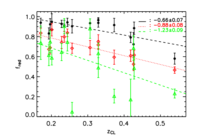
Figure 5: The red galaxy fractions for our 16 clusters using (1) galaxies in the identified cluster main-groups, displayed as solid circles; cluster galaxies (2) within 1 $R_{200}$, presented as open diamonds; and (3) at 1-1.5 $R_{200}$, plotted as triangles. A linear fit between $f_{red}$ and cluster spectroscopic redshift is performed for each sample, with the slope and its uncertainty indicated on the plot.

In Figure 5 we plot the $f_{red}$ of each cluster versus its spectroscopic redshift for different cluster-centric radii. We also overlay the results of linear fitting between $f_{red}$ and redshift. Figure 5 shows that there is a dependence of $f_{red}$ on the cluster-centric radius. The $f_{red}$ computed using galaxies in the cluster main-group have the largest values, and this subsample also exhibits the most gentle gradient. The $f_{red}$ for all three counting radii show a decreasing trend with redshift. It was shown in Ellingson et al. (2001) that the Butcher-Oemler effect is not significant within $0.5R_{200}$; our result of Figure 5 is consistent with their work. For $z<0.40$, $f_{red}$ is essentially constant for the cluster main-groups (i.e., in the cluster core), but at higher redshift there appears to be a drop in the distribution of $f_{red}$, with two out of the four clusters at $z>0.40$ having $f_{red}$ significantly lower than the values from the low-redshift clusters. This result can be interpreted as the $f_{red}$ in the cores of clusters reaching a ‘saturation’ value close to 1 at $z\sim 0.4$, while the Butcher-Oemler effect continues to be observed further out in radius.

We note that the $f_{red}$ in the core of MS0451–03, at $z=0.539$, is a significant outlier, in that its value is comparable to those at larger radii. This is likely a stochastic effect due to cosmic variance and not a general redshift trend, as the other CNOC1 cluster at the same redshift, MS0016+16 (for which we do not have photometric redshift data), shows a considerably higher red galaxy fraction in the core, derived using the CNOC1 spectroscopic data, than that of MS0451-03 (see Ellingson et al., 2001). A sudden change in the average core red fractions of clusters is not seen in the large sample of clusters at $0.45<z<0.90$ by Loh et al. (2008), further suggesting that MS0451–03 is significantly bluer in the core than the average for clusters at this redshift.

8.2 The Butcher-Oemler Effect and Stellar-Mass Selected Samples

The Butcher-Oemler effect has brought much debate in the literature since its first study in 1984 (e.g., Margoniner et al., 2001; Metevier et al., 2000; De Propris et al., 2004; Tran et al., 2005; Loh et al., 2008; Nuijten et al., 2005). The most controversial one is its existence: whether the Butcher-Oemler effect is a real phenomenon or simply due to sample selection effects (e.g., Andreon & Ettori, 1999; Andreon et al., 2004). For example, there are studies showing that the Butcher-Oemler effect becomes insignificant when the galaxy sample is selected using K-band luminosity (e.g., De Propris et al., 2003). More recently, Holden et al. (2007), using a small sample of 5 rich clusters with $0.02<z<0.9$ and sampling with a relatively high stellar-mass limit of 10${}^{10.6}M_{\sun}$, concluded that while the Butcher-Oemler effect is seen in a luminosity-selected cluster galaxy sample, a stellar-mass selected sample show insignificant changes in the galaxy red fraction over the redshift range.

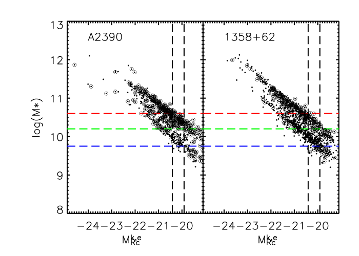
Figure 6: The estimated stellar mass M_∗ as a function of $M_{Rc}^{k,e}$ for Abell 2390 and MS1358+62. The dots are all cluster galaxies in the patch and the open circles mark those within 1$R_{200}$ of the cluster center. The vertical dashed lines indicate $M_{Rc}^{*}+1.0$ and $M_{Rc}^{*}+1.5$. The horizontal dashed lines mark log M_∗ = 9.75, 10.2, and 10.6, respectively, increasing from the bottom.

To examine this issue, we investigate the effect of stellar-mass selection on the Butcher-Oemler effect for the CNOC1 sample. We derive the stellar mass in solar units, M_∗, for galaxies in the cluster galaxy sample by applying the algorithm in Bell et al. (2003). Holden et al. (2007) used the same method, and provided a detailed discussion of the robustness and uncertainties in the derived stellar mass. We use the relation: log$({\rm M}_{*}/L_{Rc})$ = –0.523 + 0.686($M_{B}$ - $M_{Rc}$) from Bell et al. (2003) with the values of the solar units from Worthey (1994). Both $M_{Rc}$ and $M_{B}-M_{Rc}$ in our computation are k-corrected using color-dependent k-corrections (see $\S$3.2). We note that using the redder $Rc$-band luminosity, compared to the $B$ band which was used by Holden et al. (2007), produces more robust mass estimates with less scatter. As examples, we present in Figure 6 the relationship between $M_{Rc}^{k,e}$ and stellar mass for Abell 2390 and MS1358+62. In the Figure we also show lines marking the $M_{Rc}^{k,e}$ sampling limits of $M^{*}_{R_{c}}+1.0$ and $M^{*}_{R_{c}}+1.5$, and stellar mass cuts at log M_∗ = 10.6, 10.2, and 9.75. We note that the mass cuts at 10^10.2 and 10^9.75 $M_{\sun}$ correspond approximately to the average stellar mass for red and blue galaxies at $\sim M^{*}_{R_{c}}+1.5$, respectively; whereas a stellar mass of 10^10.6$M_{\sun}$ coincides with red galaxies at $\sim M^{*}_{R_{c}}+1.0$. Other clusters have remarkably similar plots, with the major difference being the completeness level (with most lower redshift clusters being considerably more complete than $M^{*}_{R_{c}}+1.5$). The most incomplete cluster is MS0451-03, which is complete to about $M^{*}_{Rc}+1.2$. We note that our $w_{i}$ and $R_{w}$ correction factors partially alleviate this problem.

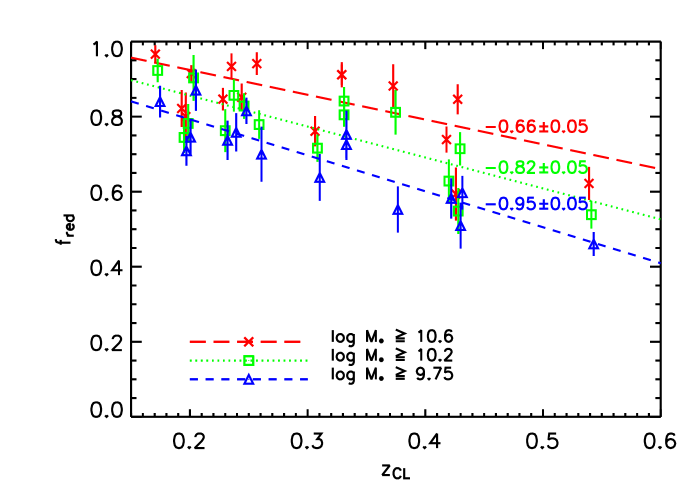
Figure 7: The $f_{red}$ for galaxies within 1$R_{200}$ of each cluster as a function of redshift. Results using three different stellar-mass (M_∗) limits are shown. A linear fit between $f_{red}$ and cluster spectroscopic redshift is performed for each sample, with the slope and its uncertainty indicated on the plot.

Using the stellar-mass selected sample for galaxies within 1$R_{200}$, we re-derive $f_{red}$ using a statistical background subtraction method similar to that for the luminosity-selected sample. Note that because of the considerably larger uncertainties in the photometric redshifts of the control sample galaxies, the derived stellar-mass measurements are expected to have significantly larger scatter. We show the results in Figure 7, where we plot the red galaxy fractions for the three different stellar-mass cuts. All three samples show the Butcher-Oemler effect, with the lower mass limit sample showing the largest change in $f_{red}$ with redshift. We note that there is significant incompleteness in the red galaxies for the higher redshift clusters for the lowest mass cut (log$M_{*}$ = 9.75) where our incompleteness correction procedure may not be effective and hence may produce smaller $f_{red}$ for the higher-redshift clusters. However, the log M_∗ = 10.2 sample, which is largely complete, also shows that a lower mass cut produces a more significant Butcher-Oemler effect. The result with the log M_∗ $\geq$ 10.2 sample is essentially identical to that in Figure 5 (open diamonds, using galaxies inside 1$R_{200}$ with a luminosity limit of $\sim M^{*}_{Rc}+1.5$), except for a systematic shift to slightly higher average $f_{red}$ values, which is due to the larger number of red galaxies in the sample when a stellar-mass cut is used.

Our sample shows that the slope of the $f_{red}$-$z$ trend is significantly shallower when using a higher stellar-mass limit. This is not a surprising conclusion, and is expected from the well-established observations pointing to the down-sizing scenario of galaxy evolution (e.g., Cowie et al., 1996; De Lucia et al., 2006; Kodama et al., 2004; Lilly et al., 2003) and the build-up of the faint end of the red sequence with decreasing redshift (e.g., Gilbank et al., 2008; van den Bosch et al., 2008; De Lucia et al., 2007; Tanaka et al., 2005; De Lucia et al., 2004). Both of these phenomena would naturally reduce the observed Butcher-Oemler effect, if the chosen sample has too high a limit in stellar mass or luminosity. Hence, the lack of strong evolution in the Holden et al. (2007) result may arise from their relatively high stellar-mass limit. The small sample size of 5 clusters used by Holden et al. also makes detecting a reduced Butcher-Oemler effect more difficult. Furthermore, the Holden et al. results are based on cluster galaxies within a cluster-centric radius of 1.25Mpc, likely significantly smaller than the $R_{200}$ radii of these rich clusters. This will also further reduce the detectability of the Butcher-Oemler effect.

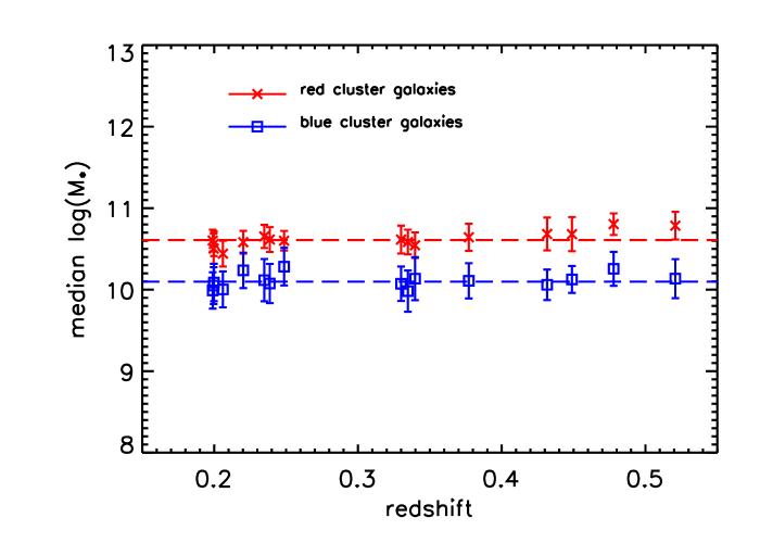
Figure 8: The median stellar mass as a function of redshift for red and blue galaxies in the clusters. Galaxies are selected within 1$R_{200}$ and in the absolute magnitude range $M^{*}_{Rc}+0.5\leq M^{k,e}_{Rc}\leq M^{*}_{Rc}+1.5$. Red galaxy samples are represented by crosses, and blue galaxy samples by open squares. These median stellar-mass values provide relative estimates of the stellar-mass limits for the red and blue galaxies in the cluster sample at the luminosity limit of $M^{*}_{Rc}+1.5$. The horizontal dashed lines show the median of the values from all the clusters. The stellar-mass limits are similar for all the clusters in the sample. The small increases seen in the limits for the highest redshift clusters are due to slight incompleteness in absolute magnitude.

Figure 6 also demonstrates that a sample chosen using a SED-dependent k- and evolution-corrected luminosity limit can in fact provide an unbiased measurement of the Butcher-Oemler effect, if this effect is generalized to mean the evolution of the color fraction of galaxies. For a chosen $M_{Rc}^{k,e}$ limit, there would be different limits for the average stellar mass for the red sequence galaxies and for the blue galaxies. As long as these mass limits do not change as a function of redshift, an $M_{Rc}^{k,e}$-selected sample essentially samples similar galaxies over the redshift range, and hence the evolution of $f_{red}$ is not driven by selection effects. As an example, for the CNOC1 sample presented here, our k- and evolution-corrected $M_{Rc}^{k,e}$ limit samples red and blue galaxies to stellar-mass limits of log M_∗ of $\sim$ 10.2 and 9.75, respectively, for all our clusters. Figure 8 plots the median stellar mass in the magnitude bin $M^{*}_{R_{c}}+0.5<M_{Rc}^{k,e}<M^{*}_{R_{c}}+1.5$ for the red and blue cluster galaxy samples as a function of cluster redshift. This illustrates that there is no substantial selection effect in the stellar mass sampled as a function of redshift. The somewhat higher mass value for MS0451-03 is due to incompleteness in $M_{Rc}^{k,e}$ in the highest redshift cluster.

In the remainder of the paper, we analyze the cluster galaxy stellar population using the luminosity-selected sample defined in $\S$3.2, which is equivalent to sampling mass limits of log M_∗ = 10.2, and 9.75 for red and blue galaxies, respectively. This allows for a more robust background subtraction based on observed magnitudes, and also increases the number of galaxies used in deriving the various statistics.

8.3 Cluster Galaxies

In this subsection, we examine the dependence of galaxy populations on redshift, $r_{CL}$, and $\Sigma_{5}$ using samples of galaxies combined from the different clusters. The cluster galaxies are separated into three redshift bins: $0.15<z<0.30$, $0.30\leq z<0.40$, and $0.40\leq z<0.55$, with 8, 4, and 4 clusters in each bin, respectively.

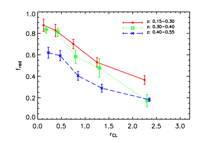
Figure 9: The $f_{red}$ as a function of $r_{CL}$ in three redshift bins, as indicated on the plot. The $r_{CL}$ values in each redshift bin are shifted slightly to provide clarity. Galaxies in all $\Sigma_{5}$ regions are included.

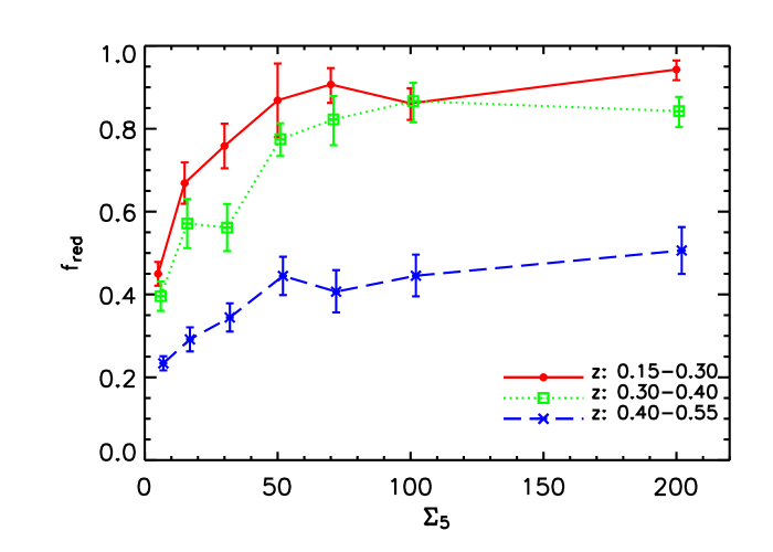
Figure 10: The $f_{red}$ as a function of $\Sigma_{5}$ in three redshift bins, as indicated on the plot. The $f_{red}$ increases with increasing $\Sigma_{5}$ in all three redshift bins.

We plot in Figure 9 the radial dependence of $f_{red}$ at each redshift bin using galaxies in all local density environments. As expected, there is a strong radial dependence of $f_{red}$ on cluster-centric radius for all redshift bins. Furthermore, we see a Butcher-Oemler effect at all radii between the high- and low-redshift bins. Figure 10 shows $f_{red}$ as a function of $\Sigma_{5}$ in each redshift bin using all cluster galaxies within $r_{CL}\leq 3R_{200}$. The galaxy red fraction in general increases with $\Sigma_{5}$. This is consistent with the well-established observational trend that that early-type, non-star-forming galaxies tend to populate high $\Sigma_{5}$ regions, while late-type, star-forming galaxies are more common in low $\Sigma_{5}$ regions (e.g., Dressler, 1980; Kodama et al., 2001; Cooper et al., 2007; Holden et al., 2007; Gómez et al., 2003; Blanton et al., 2005). Figure 10 also shows that the magnitude of the Butcher-Oemler effect depends on the local galaxy density. The high-density regions show a stronger increase in $f_{red}$ as a function of redshift, with the highest $\Sigma_{5}$ bins reaching the nominal ‘saturation’ $f_{red}$ values close to 1 at $z\sim 0.40$; whereas the lower density bins show a progressive increase in $f_{red}$ over the whole redshift range. The trend in Figure 10 can be interpreted as galaxies in higher and higher density regions completing their star formation (or have their star formation quenched) at earlier and earlier epochs. For example, galaxies with $\Sigma_{5}\geq 100$ reach $f_{red}\sim 0.9$ by $z\sim 0.35$, while those with $50\leq\Sigma_{5}<100$ become mostly red the lower redshift of $\sim 0.20$.

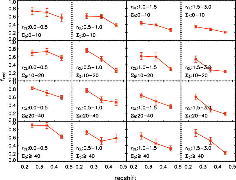
Figure 11: The ‘$f_{red}$-z’ trends in different environments, where $r_{CL}$ increases from the left to the right and $\Sigma_{5}$ increases from the top to the bottom. The general trend of $f_{red}$ decreasing with increasing redshift is seen in all panels.

Because the apparent effects of $r_{CL}$ and $\Sigma_{5}$ are largely degenerate, we probe the change in $f_{red}$ in different environments in more detail by computing its values in bins of $\Sigma_{5}$ within a fixed $r_{CL}$ location, and as a function of redshift. We divide the data into bins with $r_{CL}<0.50$, $0.50\leq r_{CL}<1.0$, $1.0\leq r_{CL}<1.5$, and $1.5\leq r_{CL}<3.0$. The data are also separated into bins of $0\leq\Sigma_{5}<10$, $10\leq\Sigma_{5}<20$, $20\leq\Sigma_{5}<40$, and $\Sigma_{5}\geq 40$. Figure 11 presents the ‘$f_{red}$-z’ trend in each $r_{CL}$ and $\Sigma_{5}$ bin. In all but one panel, $f_{red}$ declines with increasing redshift, indicating that within the uncertainties of the data the Butcher-Oemler effect is observed over the whole ranges of $r_{CL}$ and $\Sigma_{5}$ values. At large cluster-centric radii, we see that the Butcher-Oemler effect becomes progressively steeper with increasing local galaxy density. In contrast, in the cluster core the galaxy populations are dominated by red galaxies over most redshift bins, and show little evolution for $z<0.35$ for all local densities.

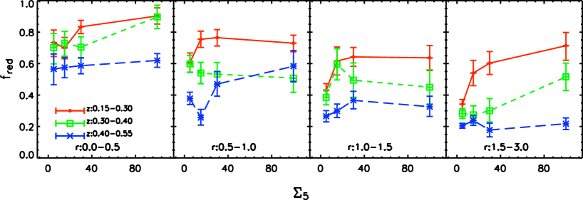
Figure 12: The ‘$f_{red}$-$\Sigma_{5}$’ trends in different $r_{CL}$ and redshift bins. The trend of $f_{red}$ increasing with $\Sigma_{5}$ is relatively weak compared to those in Figure 10. This trend is most apparent at low redshift and at large $r_{CL}$.

We examine the effect of local galaxy density on $f_{red}$ further in Figure 12, where we plot the $f_{red}$ as a function of $\Sigma_{5}$ (the ‘$f_{red}$-$\Sigma_{5}$’ trend) in different $r_{CL}$ and redshift bins. In general we find an increase of $f_{red}$ with increasing $\Sigma_{5}$, as expected from previous studies. However, the magnitude of the effect appears to be weak, and dependent on both the cluster-centric radius and the redshift. At each redshift, the slope of the ‘$f_{red}$-$\Sigma_{5}$’ trend is steepest at the outskirts ($1.5<r_{CL}<3.0$), and very weak or non-existent for galaxies within the virial radius of the clusters. An interesting observation is that the overall increase in $f_{red}$, as one moves from the outer radial bins to the inner ones, is greater than, or comparable to, the increase in $f_{red}$ as a function of $\Sigma_{5}$ over the entire local galaxy density range. This, along with the general lack of a strong dependence of $f_{red}$ on $\Sigma_{5}$ in the inner parts of the clusters, implies that the influence of the global cluster environmental, rather than the local galaxy density effect, dominates inside the cluster virialized region. Compared with the strong ‘$f_{red}$-$\Sigma_{5}$’  trends shown in Figure 10, the weak correlations of $f_{red}$ with $\Sigma_{5}$ seen when the data are divided into $r_{CL}$ bins (Figure 12) suggest that at least part of the $f_{red}$-$\Sigma_{5}$ dependence in Figure 10 is the result of a cluster-centric radius effect, since galaxies in high-density regions have a higher chance of being found in small $r_{CL}$ locations.

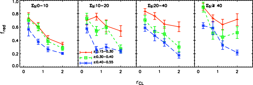
Figure 13: The ‘$f_{red}$-$r_{CL}$’ trends in different $\Sigma_{5}$ and redshift bins. The trend with $r_{CL}$ is strongest in the $\Sigma_{5}$=0–10 bin and for the high-redshift subsample in the other $\Sigma_{5}$ bins.

In Figure 13, we plot $f_{red}$ as a function of $r_{CL}$ in different redshift bins to examine more explicitly the effect of the global cluster environment on galaxies, with the local galaxy density controlled. We find that, in general, $f_{red}$ decreases with increasing $r_{CL}$ for all local densities. For the two lower-redshift samples, high $\Sigma_{5}$ regions have, on average, flatter ‘$f_{red}$-${r_{CL}}$’ trends than those for the low local density bins. However, the ‘$f_{red}$-${r_{CL}}$’ trends for the high-redshift sample are relatively steep for all the density bins. This indicates that, over our redshift range, the apparent effect of the global cluster environment is strongest in low local-density regions. This result suggests that galaxies in high local-density regions (e.g., galaxy groups) are likely to be already in a more advanced evolutionary stage, i.e., with large $f_{red}$, before infalling into the cluster, and hence the global effect of the cluster on their $f_{red}$ would be less apparent.

8.4 Cluster Galaxies in Galaxy Groups

From the results of §8.3, it is apparent that cluster galaxies in high local density regions have a different evolutionary history from those in low-density environments; however, there is also evidence that the observed galaxy density may not be the primary parameter producing these effects. High galaxy density regions outside the cluster core are often indications of galaxy groups; therefore, it is useful to attempt to delineate the effects of a group environment from those of a high local galaxy density environment.

To probe the role of galaxy groups in the evolution of cluster galaxies, we flag cluster galaxies into ‘group’ and ‘non-group’ cluster galaxies according to the pFoF group finding results (see $\S$ 5.2). Group cluster galaxies are the cluster galaxies classified as the members of pFoF groups of $N_{gal}\geq 8$ and $N_{gz}\geq 7$, and non-group cluster galaxies are those considered by the group-finding algorithm to be in pFoF groups with $N_{gal}\leq 2$ and $N_{gz}\leq 2$. Recall that the pFoF algorithm assigns a “group” membership to all galaxies, including isolated galaxies (which are assigned to groups with one member). The gaps in the $N_{gal}$ and $N_{gz}$ cutoffs serve to reduce the ambiguity in the group membership of the galaxies. The relatively high $N_{gal}$ criterion, which corresponds to a halo mass of $\sim 3.7\times 10^{13}$${\rm M}_{\odot}$, is chosen so that the group sample has an acceptable false detection rate of $<10$%. The low $N_{gal}$ criterion ensures that the non-group cluster galaxies are relatively isolated and in subhalos with no more than two galaxies brighter than $M^{*}_{R_{c}}+2.0$. Scaling with $N_{gal}$, we expected these galaxies to be in halos with mass less than $10^{13}$${\rm M}_{\odot}$. The pFoF groups with 3 to 7 members (the ‘in-between’ sample) are less well defined, as they have high false detection rates, ranging from 70% to 20%. These groups are expected to have a broad halo mass distribution, from that of a single galaxy to $\sim 3\times 10^{13}$${\rm M}_{\odot}$. The cluster galaxies associated with the cluster main-groups are excluded from the group cluster galaxies, so that the environmental effects caused by galaxy groups can be specifically investigated. We can consider that cluster main-group galaxies are the galaxies residing in the core of the main dark matter halo which defines the cluster.

We have a total of 1073, 1226 and 3507 cluster galaxies in the cluster main-group, group, and non-group subsamples, respectively. A total of 5727 galaxies fall in between the group and non-group criteria. It is interesting to note that with this subdivision of cluster galaxies, we find that $\sim 17.5$% of the galaxies outside the virial radius ($>1R_{200}$) are in subhalos with masses greater $\sim 3$–$4\times 10^{13}$${\rm M}_{\odot}$. This is broadly consistent with the simulations of Berrier et al. (2009) which found $\sim$15% of galaxies in their most massive clusters (which are most comparable with the CNOC1 sample) are accreted from groups with halo masses larger than $\sim 3.5\times 10^{13}$${\rm M}_{\odot}$.

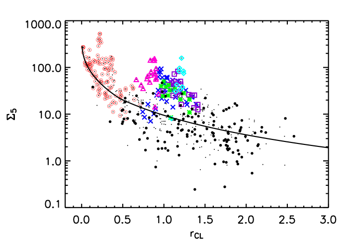
Figure 14: Local galaxy density $\Sigma_{5}$ as a function of cluster-centric radius $r_{CL}$ in units of $R_{200}$ using Abell 2390 cluster galaxies. The crosses, squares, triangles, stars, and diamonds represent group galaxies in different cluster groups (see Figure 3). The thick solid circles are the ‘non-group’ cluster galaxies and those marked with large open circles are the cluster galaxies in the cluster main-group. The small dots are those in between our ‘group’ and ’non-group’ categories. In general, the group galaxies populate regions of $\Sigma_{5}$ relatively higher than those of the non-group galaxies. The solid curve is the projected NFW profile fitted using the cluster main-group and non-group galaxies.

We illustrate in Figure 14 an example of the distributions of the three subsamples of cluster galaxies in the $\Sigma_{5}$-$r_{CL}$ plane using Abell 2390. For completeness, the ‘in-between’ sample (between those considered to be group cluster and non-group cluster galaxies) is also plotted. The $\Sigma_{5}$ distribution can be described in general as having a decreasing envelope with increasing radius, with high-density groups super-imposed on it. The envelope distribution can be fitted reasonably well with a projected NFW (Navarro et al., 1996) profile. It is interesting to note that Figure 14 demonstrates that the $\Sigma_{5}$ measurements computed using photometric redshifts can produce a reasonable projected galaxy density profile for the cluster, indicating that these density measurements are in fact physically meaningful, at least when considered over a factor of several in density.

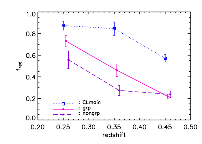
Figure 15: The ‘$f_{red}$-z’ trends for the cluster main-group, group cluster, and non-group cluster galaxies as indicated on the plot, using galaxies in all $\Sigma_{5}$ bins. All group and non-group galaxies are located at $r_{CL}<3$. The cluster main-group subsample has the largest $f_{red}$, while the non-group galaxies exhibit a weak ‘$f_{red}$-z’ trend.

Figure 15 shows the redshift dependence of $f_{red}$ for the three subsamples of galaxies inside $r_{CL}$=3, using galaxies in all local galaxy density environments. We see that all three samples show an increase of $f_{red}$ with decreasing redshift, but have systematically different levels of $f_{red}$, with the cluster main-group being the reddest and the non-group cluster galaxies the bluest. Furthermore, the three subsamples also show different evolution in $f_{red}$. The cluster main-group galaxies exhibit the largest $f_{red}$ and reach the final state of $f_{red}\sim 1$ earlier than the group cluster galaxies. The group cluster galaxies show the strongest evolution from $z\sim 0.5$ to 0.2, reaching $f_{red}$ close to that of the cluster main-group galaxies at the low-redshift bin. The non-group cluster galaxies, located in less massive subhalos, show a milder increase in $f_{red}$, still retaining a substantial fraction of blue galaxies in the low-redshift bin. They begin to partake in significant evolution at the lower redshift of $z\sim 0.35$. In the context of the halo model, the cluster cores are the center of the most massive dark matter halos, while group and non-group cluster galaxies are in successively less massive subhalos. The epoch when $f_{red}$ reaches $\sim 1$ is therefore a reflection of the dependence of galaxy evolution on the halo mass: galaxies in more massive halos have their star formation truncated at an earlier time than do those in less massive halos. This result can be described as a ‘group down-sizing’ effect, akin to the down-sizing effect seen in the evolution of individual galaxies (e.g., Cowie et al., 1996; Cattaneo et al., 2008; Seymour et al., 2008), though the physical mechanisms underlying this effect may be very different.

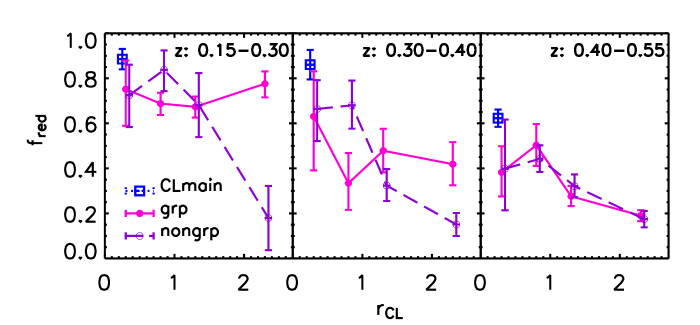
Figure 16: The ‘$f_{red}$-$r_{CL}$’ trends in different redshift bins for the three subsamples indicated on the plot. Group cluster galaxies outside $\sim 1R_{200}$ evolve much more rapidly than non-group cluster galaxies over this redshift range.

Figure 16 demonstrates the different evolutionary histories of galaxies in subhalos of different sizes by plotting the dependence of $f_{red}$ on cluster centric radius for the three galaxy subsamples in different redshift bins. We plot the cluster main-groups as a single point at a small radius. Cluster galaxies in groups show the largest increases in $f_{red}$ with decreasing redshift; and this increase is seen in both inner and outer cluster-centric radius bins. The $f_{red}$ for galaxies in groups in the cluster outskirts shows the largest change with redshift, catching up to the value of the cluster main-group galaxies in the core by $z\sim 0.2$, by which time a flat $f_{red}$ distribution in cluster-centric radius is seen. In comparison, the $f_{red}$ of non-group cluster galaxies shows a very strong radial gradient at the low-redshift bin. The rate of evolution of $f_{red}$ for the non-group cluster galaxies depends significantly on the cluster-centric radius, such that galaxies in the outermost radial bin (at $\sim 2R_{200}$) show little change with redshift, while galaxies near $R_{200}$ evolve significantly.

Our results suggest that galaxies in moderately massive groups outside of the cluster core are turning red in response to the environment of their own dark matter subhalos, with the cluster environment having a strong effect possibly only at the core. On the other hand, the non-group cluster galaxies, situated in low mass subhalos, appear to turn red at a low or non-existent rate at the outskirts, and significant evolution is seen only when they are near the virial radius of the cluster. This result can be interpreted as galaxies in small subhalos being much more affected by the massive cluster dark matter halo into which they are falling. However, another possible contribution to this increase of $f_{red}$ for the non-group sample near the virial radius could come from member galaxies of more massive infalling groups (which have already turned red), which have been dynamically stripped from their parent subhalos.

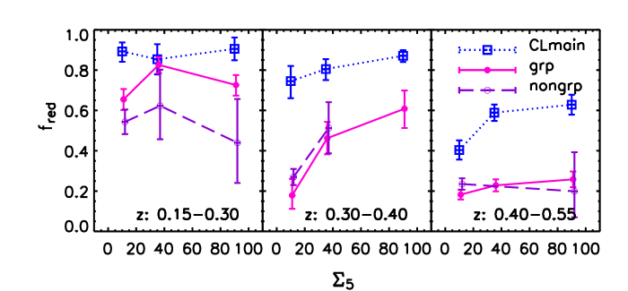
Figure 17: The ‘$f_{red}$-$\Sigma_{5}$’ trends in different redshift bins for the three subsamples indicated on the plot.

To separate the effects of local galaxy density and group membership, we plot in Figure 17 $f_{red}$ for the three subsamples at different redshifts as a function of $\Sigma_{5}$. The uncertainties are fairly large due to the small sample size, but, nevertheless, the plots suggest that, after controlling for the local galaxy density, the three subsamples still have different red fractions. This result indicates that the different average local galaxy densities in these subsamples do not entirely explain the different $f_{red}$ measured. Comparing galaxies in the cluster main-groups to those in groups in the high-redshift bin, the cluster galaxies in groups have substantially smaller $f_{red}$ at all densities, similar to non-group cluster galaxies. By $z\sim 0.2$, the group cluster galaxies have evolved into having $f_{red}$ similar to the cluster main-group galaxies, while the non-group cluster galaxies show a considerably milder evolution. Thus, by $z\sim 0.2$, cluster galaxies in groups are redder than their non-group counterparts in similar local galaxy densities, implying that group membership, or more precisely, the mass of the subhalo in which a galaxy resides, has a stronger effect on the evolution of its stellar population than does the local galaxy density.

9 Discussion

The availability of photometric redshift information over a large field of view allows us to examine the Butcher-Oemler effect in galaxy clusters in detail, including investigating the effects of local galaxy density and the dependence on the global cluster scale. Furthermore, by separating the cluster galaxies into different group status categories, roughly indicative of the size of the dark matter subhalo in which they reside, we are able to examine more closely the nature of the dependence of the galaxy red fraction on their subhalo masses.

Figures 9 to 13 illustrate the apparent dependence of galaxy colors on local galaxy density and cluster centric radius, averaged over the whole cluster galaxy sample. Looking at cluster galaxies as a whole, by $z\sim 0.20$, most cluster galaxies in high $\Sigma_{5}$ regions already have their star formation truncated, as their $f_{red}$ is close to 1 (see Figure 10). The truncation process appears to occur earlier for galaxies in denser regions. Assuming a galaxy would turn red 1$\sim$2 Gyr after star formation is quenched, this truncation process is mostly completed by the redshift of $\sim 0.45$ for galaxies in high-density regions, given that their $f_{red}$ reaches $\sim$1 by our low-redshift bin ($z\sim 0.20$).

The cluster environment, as defined by the position of the galaxy in the cluster, however, appears to have an even stronger effect on $f_{red}$ than the local galaxy density. For galaxies with similar $\Sigma_{5}$, those closer to the cluster center have a larger fraction of their star formation suppressed than those in the outskirts (Figure 11, comparing within each row). When the galaxy sample is separated into subsamples in cluster-centric radius, the dependence of $f_{red}$ on the local galaxy density is considerably weaker, and nearly non-existent in the cores of clusters (Figure 12), suggesting that local galaxy density is not the dominant environmental parameter. We also find galaxies in low-density regions have a steeper $f_{red}$-$r_{CL}$ gradient, compared to those in high-density regions (Figure 13). This suggests that the effects of the global cluster environment are stronger for galaxies in low-density regions. However, an alternative interpretation might be that star formation in galaxies in high $\Sigma_{5}$ regions may have already been largely stopped by some other processes not associated with the global cluster environment; whereas in low $\Sigma_{5}$ regions, there is still a relatively large fraction of star-forming galaxies available to have their star formation truncated by the cluster environment as they approach the cluster virial region.

The weak dependence of $f_{red}$ on local galaxy density seen when the data are analyzed in different $r_{CL}$ bins (Figure 12) suggests that $\Sigma_{5}$ may not be a fundamental parameter in determining the evolution of the galaxy population in clusters. Separating cluster galaxies into group and non-group galaxies, representing galaxies in more and less massive subhalos, provides us with additional insights into cluster galaxy population evolution, and a more physical interpretation of the apparent dependence on local galaxy density. The dependence of $f_{red}$ on $\Sigma_{5}$ for both group and non-group cluster galaxies is also weak (Figure 17), similar to that found for the (whole) cluster galaxy sample after they are separated into bins of cluster-centric radii (Figure 12). The most significant result from applying the group and non-group selection of galaxy subsamples is presented in Figure 16. It presents clear evidence that, outside the cluster core, galaxies situated in the more massive subhalos (the group cluster galaxies) have a much stronger Butcher-Oemler effect, regardless of their position relative to the cluster center. In the context of a dark matter halo model, this suggests that much of the dependence of the galaxy population on local galaxy density can be attributed to whether an infalling cluster galaxy is in a massive subhalo.

Our analysis shows that cluster galaxies in groups, regardless of their local galaxy density and cluster-centric radius, exhibit a much stronger Butcher-Oemler effect than the non-group cluster galaxies (Figure 16 and 17); the difference between these subsamples is especially large beyond the virial radius. In fact, the cluster galaxies considered to be in moderately massive subhalos appear to be the most significant contributors to the observed Butcher-Oemler effect at the cluster outskirts ($\sim 2-3R_{200}$) over the redshift range of our sample. This dependence on halo mass can also be extended to include the core of a cluster, which is the center of the most massive halo. The cores of the clusters have high red fractions close to 1 at $z\sim 0.4$; they complete the quenching of star formation the earliest, ahead of the less massive infalling subhalos.

The evolution of $f_{red}$ of the large sample of cluster galaxies with pFoF group membership falling in between the group cluster and non-group cluster galaxies is also consistent with this picture. This sample contains the bulk of the cluster galaxies – about 49% of the cluster galaxies outside the cluster core. The $f_{red}$ of this sample at the outer cluster-centric radial bins show a Butcher-Oemler effect that is between those of the group cluster and non-group cluster galaxies. For example, at the outermost $r_{CL}$ bin, $f_{red}$ rises from $0.19\pm 0.02$ at $z\sim 0.4$ to $0.42\pm 0.06$ at $z\sim 0.2$. It is more difficult to quantify the halo mass of objects in this sample because of the high false group detection rate (see §8.4). This sample is expected to contain a broad mix of subhalo masses, with very roughly half of the galaxies being in subhalos with masses of $\sim 1-3\times 10^{13}$${\rm M}_{\odot}$, and the other half, being contaminated by projections, residing in subhalos of smaller masses, similar to those in the non-group cluster galaxy sample. The more massive subhalos in this sample, along with the group cluster galaxy sample, could represent a total of 30 to 45% of all the the infalling cluster galaxies. They are likely the main contributors to Butcher-Oemler effect seen in the outer radial bins.

This rapid evolution of group populations at $z\sim 0.3$, combined with the red cores of clusters seen at higher redshifts and the bluer colors of galaxies in smaller groups, implies that galaxies in the most massive halos (i.e., in the cluster cores) have star formation quenched at an earlier time than those in moderately massive infalling groups. These, in turn, become red at an earlier time than the non-group galaxies residing in yet less massive subhalos (Figure 12). This effect suggests that mechanisms responsible for the truncation of star formation in galaxies in more massive halos operate more efficiently, or become more effective in earlier epochs.

Related to the more rapid evolution of $f_{red}$ in group galaxies is the ‘pre-processing’ effect on galaxies in infalling groups, suggested by number of previous studies (e.g., Blake et al., 2004; Tanaka et al., 2005; Cooper et al., 2008; McIntosh et al., 2008). We clearly observe this in Figure 16, as the $f_{red}$ of galaxies in groups increases with decreasing redshift at all cluster-centric radii. The pre-processing effect is essentially a manifestation that the more massive subhalos in a cluster have a dominant effect on their galaxy populations, producing a strong Butcher-Oemler effect regardless of their distance from the cluster center. By $z\sim 0.35$, this ‘processing’ of galaxies in moderately massive subhalos results in galaxies which are redder than the non-group galaxies in similar local galaxy density regions located at similar cluster-centric radii. The $f_{red}$ of these galaxies, even at large $r_{CL}$, becomes similar to that of the evolved galaxies in the cluster core by $z\sim 0.2$. While our sample demonstrates this effect in groups with subhalo masses larger than $\sim 3-4\times 10^{13}$ ${\rm M}_{\odot}$, it also likely occurs in subhalos 2 or 3 times less massive. This increase in the dominance of red galaxies in groups appears to be a significant, if not the primary, contributor of the Butcher-Oemler effect over the redshift range of 0.5 to 0.2. The increase of $f_{red}$ for the galaxies in both the non-group cluster galaxies and the cluster core galaxies is considerably smaller over this redshift range, in that the galaxies in the cluster core have already completed their evolution, and small subhalos (hosting the non-group cluster galaxies) outside the core still contain a substantial number of blue galaxies even at $z\sim 0.2$.

10 Conclusions

We have investigated the environmental effects on the properties of the CNOC1 cluster galaxies at $0.17<z<0.55$ using both individual galaxies and those in galaxy groups, utilizing photometric redshift data covering a relatively large field out to 2 – 3 $R_{200}$. We use local projected galaxy density, $\Sigma_{5}$, and cluster-centric radius, $r_{CL}$, in units of $R_{200}$ as proxies for the local and global environment, and adopt the red galaxy fraction, $f_{red}$, as the measurement of galaxy population properties. We summarize our results as follows:

1.) The Butcher-Oemler effect is observed in all $r_{CL}$ and $\Sigma_{5}$ bins between redshifts of 0.5 and 0.2 (Figure 11). However, the change of $f_{red}$ in the cluster core (less than 0.5 $R_{200}$) is minimal at $z<0.4$, suggesting that the truncation of star formation in the center of the most massive halos occurred at earlier epochs.

2.) We find that stellar-mass selected samples also show the Butcher-Oemler effect. Comparing the samples selected using different stellar-mass limits (at 1 $R_{200}$), we find the steepness of the Butcher-Oemler effect to be dependent on the stellar-mass limit. A sample selected using a higher stellar-mass limit has a milder change in $f_{red}$ compared to one with a lower stellar-mass limit.

3.) There are apparent correlations between $\Sigma_{5}$ and $f_{red}$ in all our three redshift bins. However, the dependence of $f_{red}$ on local galaxy density becomes much weaker when the galaxy sample is separated by cluster-centric radius or group/non-group status, with the possible exception at the cluster outskirts. This suggests that local galaxy density may not be the primary environment parameter affecting the average galaxy population.

4.) We separate the cluster galaxies into three subsamples: cluster main-group, group cluster, and non-group cluster galaxies, roughly representing galaxies situated in the core of the massive dark matter halo of the cluster, in moderately massive subhalos, and in low-mass subhalos, respectively. These three samples have different $f_{red}$ values and rates of change of $f_{red}$ with redshift. Galaxies in the central massive cluster halo reach $f_{red}\sim 1$ at a larger redshift than those in galaxy groups, which in turn reach $f_{red}\sim 1$ at an earlier time than the non-group galaxies. This suggests that the dominant determinant of the epoch of the quenching of star formation is the mass of the dark matter subhalos in which the galaxy resides. The apparent correlation between $\Sigma_{5}$ and $f_{red}$ is at least in part due to the correlation of high local galaxy density with the presence of a massive halo. The epoch when $f_{red}$ in a galaxy group reaches the evolved stage of $f_{red}\sim 1$ depends on the halo mass.

5.) We find that galaxy groups falling into a cluster ‘process’ galaxies therein and turn them red at an earlier time; what is termed as ‘pre-processing’. This is observed even after controlling for $\Sigma_{5}$. Such ‘pre-processing’ is seen for groups at the outer $r_{CL}$ and the cluster outskirts. By $z\sim 0.20$, galaxies in groups have a high red fraction, similar to that in the cluster core, regardless of their cluster-centric radius. This more rapid evolution of galaxies in infalling moderately rich groups appears to be a significant contributor to the Butcher-Oemler effect.

Some of our analyses and interpretations are tentative and suggestive, based on a small-size sample of 16 clusters and 89 cluster groups. The completion of the Red-sequence Cluster Survey 1 and 2 (RCS; Hsieh et al., 2005; Yee et al., 2007) promises to provide similar data for thousands of clusters, providing greatly improved statistics to investigate the roles of dark matter halo environment on galaxy evolution.

Table 1: Properties of CNOC1 Follow-up Data Set

Cluster	R.A.(J2000)	Dec.(J2000)	$z_{spec}$	$m_{R_{c},lim}$	seeinga	note
MS0302+16	03:05:18.1	17:28:24.9	0.425	24.10	0.70	classical
						not a CNOC1 cluster
CL0303+17	03:06:18.7	17:18:03.0	0.418			S-E field
						not a CNOC1 cluster
MS0440+02	04:43:09.9	02:10:21.4	0.197	23.71	0.58	classical
MS0451+02	04:54:14.1	02:57:10.5	0.201	23.72	0.68	classical
MS0451-03	04:54:10.9	-03:00:57.1	0.539	22.80	1.11	classical
MS0839+29	08:42:55.9	29:27:27.3	0.193	23.05	0.86	classical
MS0906+11	09:09:12.7	10:58:29.2	0.171	23.03	0.82	classical
MS1008-12	10:10:32.3	-12:39:52.5	0.306	23.35	1.17	classical
MS1224+20	12:27:13.3	19:50:56.5	0.330	21.70		queue, not use
MS1231+15	12:33:55.4	15:25:59.1	0.235	23.80	0.82	queue
Abell 1560	12:34:07.1	15:10:28.2	0.244			S field
						not a CNOC1 cluster
MS1358+62	13:59:50.5	62:31:04.5	0.329	22.65	1.24	classical
MS1358+62S	13:59:38.0	62:18:47.0	0.329			S field
						not a CNOC1 cluster
MS1455+22	14:57:15.1	22:20:33.9	0.257	23.20	0.93	queue
MS1512+36	15:14:22.5	36:36:20.9	0.373	23.85	0.87	queue
MS1621+26	16:23:35.5	26:34:15.9	0.428	23.35	0.93	classical
Abell 2390	21:53:36.8	17:41:43.7	0.228	24.05	0.72	classical

Table 2: Exposure Times^b and Filters for Each Cluster

Cluster	$B$	$V$	$R_{c}$	$I$		Cluster	$B$	$V$	$R_{c}$	$I$
MS0302+16	92	20	16	16		MS1224+20	69	12	12	12
MS0440+02	20	7	7	7		MS1231+15	20	7	7	7
MS0451+02	20	7	7	7		MS1358+62	69	15	10.5	15
MS0451-03	60	69	24	24		MS1455+22	20	7	7	7
MS0839+29	20	7	7	7		MS1512+36	23	15	14	14
MS0906+11	40	7	7	14		MS1621+26	20	12	16	10
MS1008-12	44	7	14	7		Abell 2390	15	10	10	12

Table 3: Properties of pFoF Determined CNOC1 Clusters ($D0_{xy}=0.25Mpc$)

Cluster	R.A.(J2000)	Dec.(J2000)	$z_{pFoF,cl}$	$N_{gal}$	$R_{200}^{c}$	$f_{red}$
MS0302+16	03:05:18.25	17:28:29.5	$0.4488\pm 0.0095$	$27.4\pm 2.4$	1.20	$0.698\pm 0.115$
CL0303+17	03:06:19.69	17:18:29.9	$0.4778\pm 0.0045$	$135.0\pm 5.0$	2.05	$0.624\pm 0.053$
MS0440+02	04:43:09.95	02:10:21.6	$0.1989\pm 0.0032$	$29.5\pm 2.3$	1.24	$0.922\pm 0.057$
MS0451+02	04:54:13.85	02:57:07.4	$0.1998\pm 0.0005$	$208.5\pm 12.6$	1.97	$0.947\pm 0.080$
MS0451-03	04:54:12.60	-00:00:48.4	$0.5260\pm 0.0041$	$222.1\pm 12.9$	2.07	$0.357\pm 0.051$
MS0839+29	08:42:56.06	29:27:40.8	$0.1996\pm 0.0018$	$70.4\pm 2.7$	1.60	$0.831\pm 0.056$
MS0906+11	09:09:07.57	10:57:55.1	$0.2060\pm 0.0042$	$36.5\pm 2.8$	1.79d	$0.939\pm 0.045$
MS1008-12	10:10:32.45	-00:39:52.2	$0.3300\pm 0.0051$	$57.4\pm 3.6$	1.94	$0.933\pm 0.043$
MS1231+15	12:33:54.51	15:26:59.1	$0.2348\pm 0.0034$	$39.0\pm 2.5$	1.30	$0.907\pm 0.055$
Abell 1560	12:34:14.46	15:13:40.1	$0.2486\pm 0.0029$	$60.8\pm 3.4$	1.57	$0.942\pm 0.041$
MS1358+62	13:59:50.33	62:31:00.7	$0.3390\pm 0.0037$	$65.3\pm 4.2$	1.64	$0.959\pm 0.029$
MS1358+62S	13:59:34.04	62:19:05.2	$0.3347\pm 0.0040$	$53.5\pm 3.7$	1.50	$0.932\pm 0.043$
MS1455+22	14:57:11.66	22:19:54.2	$0.2386\pm 0.0051$	$33.1\pm 2.4$	2.24	$0.903\pm 0.067$
MS1512+36	15:14:22.43	36:36:23.1	$0.3771\pm 0.0093$	$15.6\pm 2.0$	1.21	$0.915\pm 0.067$
MS1621+26	16:23:35.48	26:34:52.1	$0.4315\pm 0.0033$	$42.5\pm 3.0$	1.39	$0.884\pm 0.061$
Abell 2390	21:53:37.06	17:41:17.1	$0.2202\pm 0.0012$	$126.7\pm 4.3$	2.16	$0.927\pm 0.036$

.

References

- Abell et al. (1989) Abell, G. O., Corwin, Jr., H. G., & Olowin, R. P. 1989, ApJS, 70, 1
- Abraham et al. (1996) Abraham, R. G., et al. 1996, ApJ, 471, 694
- Adami et al. (2005) Adami, C., Biviano, A., Durret, F., & Mazure, A. 2005, A&A, 443, 17
- Andreon & Ettori (1999) Andreon, S. & Ettori, S. 1999, ApJ, 516, 647
- Andreon et al. (2004) Andreon, S., Lobo, C., & Iovino, A. 2004, MNRAS, 349, 889
- Andreon et al. (2006) Andreon, S., Quintana, H., Tajer, M., Galaz, G., & Surdej, J. 2006, MNRAS, 365, 915
- Barkhouse et al. (2007) Barkhouse, W. A., Yee, H. K. C., & López-Cruz, O. 2007, ApJ, 671, 1471
- Bekki (1999) Bekki, K. 1999, ApJ, 510, L15
- Bell et al. (2003) Bell, E. F., McIntosh, D. H., Katz, N., & Weinberg, M. D. 2003, ApJS, 149, 289
- Berrier et al. (2009) Berrier, J. C., Stewart, K. R., Bullock, J. S., Purcell, C. W., Barton, E. J., & Wechsler, R. H. 2009, ApJ, 690, 1292
- Blake et al. (2004) Blake, C., et al. 2004, MNRAS, 355, 713
- Blanton et al. (2005) Blanton, M. R., Eisenstein, D., Hogg, D. W., Schlegel, D. J., & Brinkmann, J. 2005, ApJ, 629, 143
- Borgani et al. (1999) Borgani, S., Girardi, M., Carlberg, R. G., Yee, H. K. C., & Ellingson, E. 1999, ApJ, 527, 561
- Butcher & Oemler (1984) Butcher, H. & Oemler, Jr., A. 1984, ApJ, 285, 426
- Carlberg et al. (1996) Carlberg, R. G., Yee, H. K. C., Ellingson, E., Abraham, R., Gravel, P., Morris, S., & Pritchet, C. J. 1996, ApJ, 462, 32
- Carlberg et al. (1997) Carlberg, R. G., et al. 1997, ApJ, 485, L13+
- Cattaneo et al. (2008) Cattaneo, A., Dekel, A., Faber, S. M., & Guiderdoni, B. 2008, MNRAS, 389, 567
- Cooper et al. (2007) Cooper, M. C., et al. 2007, MNRAS, 224
- Cooper et al. (2008) Cooper, M. C., Tremonti, C. A., Newman, J. A., & Zabludoff, A. I. 2008, MNRAS, 1037
- Cowie et al. (1996) Cowie, L. L., Songaila, A., Hu, E. M., & Cohen, J. G. 1996, AJ, 112, 839
- Coziol & Plauchu-Frayn (2007) Coziol, R. & Plauchu-Frayn, I. 2007, AJ, 133, 2630
- D’Agostini (2004) D’Agostini, G. 2004, ArXiv Physics e-prints
- Dahlén et al. (2004) Dahlén, T., Fransson, C., Östlin, G., & Näslund, M. 2004, MNRAS, 350, 253
- David et al. (1999) David, L. P., Forman, W., & Jones, C. 1999, ApJ, 519, 533
- De Lucia et al. (2004) De Lucia, G., et al. 2004, ApJ, 610, L77
- De Lucia et al. (2007) De Lucia, G., et al. 2007, MNRAS, 374, 809
- De Lucia et al. (2006) De Lucia, G., Springel, V., White, S. D. M., Croton, D., & Kauffmann, G. 2006, MNRAS, 366, 499
- De Propris et al. (2004) De Propris, R., 2004, MNRAS, 351, 125
- De Propris et al. (2003) De Propris, R., Stanford, S. A., Eisenhardt, P. R., & Dickinson, M. 2003, ApJ, 598, 20
- Domínguez et al. (2002) Domínguez, M. J., Zandivarez, A. A., Martínez, H. J., Merchán, M. E., Muriel, H., & Lambas, D. G. 2002, MNRAS, 335, 825
- Dressler (1980) Dressler, A. 1980, ApJS, 42, 565
- Ellingson et al. (2001) Ellingson, E., Lin, H., Yee, H. K. C., & Carlberg, R. G. 2001, ApJ, 547, 609
- Fujita (2004) Fujita, Y. 2004, PASJ, 56, 29
- Gerke et al. (2007) Gerke, B. F., et al. 2007, MNRAS, 222
- Giavalisco et al. (2004) Giavalisco, M., et al. 2004, ApJ, 600, L93
- Gilbank et al. (2008) Gilbank, D. G., Yee, H.K.C., Ellingson, E., Gladders, M. D., Loh, Y.-S., Barrientos, L. F., & Barkhouse, W. A. 2008, ApJ, 673, 74
- Gladders & Yee (2005) Gladders, M. D. & Yee, H. K. C. 2005, ApJS, 157, 1
- Gómez et al. (2003) Gómez, P. L., et al. 2003, ApJ, 584, 210
- Goto et al. (2003) Goto, T., Yamauchi, C., Fujita, Y., Okamura, S., Sekiguchi, M., Smail, I., Bernardi, M., & Gomez, P. L. 2003, MNRAS, 346, 601
- Helsdon & Ponman (2003a) Helsdon, S. F. & Ponman, T. J. 2003a, MNRAS, 339, L29
- Helsdon & Ponman (2003b) —. 2003b, MNRAS, 340, 485
- Hogg et al. (2003) Hogg, D. W., et al. 2003, ApJ, 585, L5
- Holden et al. (2007) Holden, B. P., et al. 2007, ApJ, 670, 190
- Hsieh et al. (2005) Hsieh, B. C., Yee, H. K. C., Lin, H., & Gladders, M. D. 2005, ApJS, 158, 161
- Jeltema et al. (2007) Jeltema, T. E., Mulchaey, J. S., Lubin, L. M., & Fassnacht, C. D. 2007, ApJ, 658, 865
- Kodama & Arimoto (1997) Kodama, T. & Arimoto, N. 1997, A&A, 320, 41
- Kodama et al. (2001) Kodama, T., Smail, I., Nakata, F., Okamura, S., & Bower, R. G. 2001, ApJ, 562, L9
- Kodama et al. (2004) Kodama, T., et al. 2004, MNRAS, 350, 1005
- Krick et al. (2006) Krick, J. E., Bernstein, R. A., & Pimbblet, K. A. 2006, AJ, 131, 168
- Landolt (1992) Landolt, A. U. 1992, AJ, 104, 340
- Li & Yee (2008) Li, I. H. & Yee, H. K. C. 2008, AJ, 135, 809
- Lilly et al. (2003) Lilly, S. J., Carollo, C. M., & Stockton, A. N. 2003, ApJ, 597, 730
- Lin et al. (1999) Lin, H., Yee, H. K. C., Carlberg, R. G., Morris, S. L., Sawicki, M., Patton, D. R., Wirth, G., & Shepherd, C. W. 1999, ApJ, 518, 533
- Loh et al. (2008) Loh, Y.-S., Ellingson, E., Yee, H. K. C., Gilbank, D. G., Gladders, M. D., & Barrientos, L. F. 2008, ApJ, 680, 214
- Mamon (2000) Mamon, G. A. 2000, in Astronomical Society of the Pacific Conference Series, Vol. 197, Dynamics of Galaxies: from the Early Universe to the Present, ed. F. Combes, G. A. Mamon, & V. Charmandaris, 377–+
- Margoniner et al. (2001) Margoniner, V. E., de Carvalho, R. R., Gal, R. R., & Djorgovski, S. G. 2001, ApJ, 548, L143
- McIntosh et al. (2008) McIntosh, D. H., Guo, Y., Hertzberg, J., Katz, N., Mo, H. J., van den Bosch, F. C., & Yang, X. 2008, MNRAS, 388, 1537
- Metevier et al. (2000) Metevier, A. J., Romer, A. K., & Ulmer, M. P. 2000, AJ, 119, 1090
- Mulchaey & Zabludoff (1998) Mulchaey, J. S. & Zabludoff, A. I. 1998, ApJ, 496, 73
- Navarro et al. (1996) Navarro, J. F., Frenk, C. S., & White, S. D. M. 1996, ApJ, 462, 563
- Nuijten et al. (2005) Nuijten, M. J. H. M., Simard, L., Gwyn, S., & Röttgering, H. J. A. 2005, ApJ, 626, L77
- Pierre et al. (1996) Pierre, M., Le Borgne, J. F., Soucail, G., & Kneib, J. P. 1996, A&A, 311, 413
- Poggianti (1997) Poggianti, B. M. 1997, A&AS, 122, 399
- Poggianti et al. (2006) Poggianti, B. M., et al. 2006, ApJ, 642, 188
- Seymour et al. (2008) Seymour, N., et al. 2008, MNRAS, 386, 1695
- Solanes et al. (1999) Solanes, J. M., Salvador-Solé, E., & González-Casado, G. 1999, A&A, 343, 733
- Springel et al. (2005) Springel et al. 2005, Nature, 435, 629
- Tanaka et al. (2005) Tanaka, M., Kodama, T., Arimoto, N., Okamura, S., Umetsu, K., Shimasaku, K., Tanaka, I., & Yamada, T. 2005, MNRAS, 362, 268
- Tran et al. (2005) Tran, K.-V. H., van Dokkum, P., Illingworth, G. D., Kelson, D., Gonzalez, A., & Franx, M. 2005, ApJ, 619, 134
- Ulmer & Cruddace (1982) Ulmer, M. P. & Cruddace, R. G. 1982, ApJ, 258, 434
- van den Bosch et al. (2008) van den Bosch, F. C., Aquino, D., Yang, X., Mo, H. J., Pasquali, A., McIntosh, D. H., Weinmann, S. M., & Kang, X. 2008, MNRAS, 387, 79
- Verdugo et al. (2008) Verdugo, M., Ziegler, B. L., & Gerken, B. 2008, A&A, 486, 9
- Wilman et al. (2005) Wilman, D. J., Balogh, M. L., Bower, R. G., Mulchaey, J. S., Oemler, A., Carlberg, R. G., Morris, S. L., & Whitaker, R. J. 2005, MNRAS, 358, 71
- Wilman et al. (2008) Wilman, D. J., et al. 2008, ApJ, 680, 1009
- Worthey (1994) Worthey, G. 1994, ApJS, 95, 107
- Yan et al. (2008) Yan, R., et al. 2008, ArXiv e-prints
- Yee (1991) Yee, H. K. C. 1991, PASP, 103, 396
- Yee et al. (1996) Yee, H. K. C., Ellingson, E., & Carlberg, R. G. 1996, ApJS, 102, 269
- Yee et al. (2007) Yee, H. K. C., Gladders, M. D., Gilbank, D. G., Majumdar, S., Hoekstra, H., & Ellingson, E. 2007, in Astronomical Society of the Pacific Conference Series, Vol. 379, Cosmic Frontiers, ed. N. Metcalfe & T. Shanks, 103–+
- Yee et al. (2000) Yee, H. K. C., et al. 2000, ApJS, 129, 475