Photometric Variability in Earthshine Observations

The identification of an extrasolar planet as Earth-like will depend on the detection of atmospheric signatures or surface non-uniformities. In this paper we present spatially unresolved flux light curves of Earth for the purpose of studying a prototype extrasolar terrestrial planet. Our monitoring of the photometric variability of earthshine revealed changes of up to $23\%$ per hour in the brightness of Earth’s scattered light at around 600 nm, due to the removal of specular reflection from the view of the Moon. This variability is accompanied by reddening of the spectrum, and results from a change in surface properties across the continental boundary between the Indian Ocean and Africa’s east coast. Our results based on earthshine monitoring indicate that specular reflection should provide a useful tool in determining the presence of liquid water on extrasolar planets via photometric observations.

Keywords: Earthshine - photometric monitoring - Earth.

Introduction

A primary goal of future space-based missions, such as the European Space Agency’s Darwin and the National Aeronautics and Space Administration’s Terrestrial Planet Finder (TPF), is the discovery of planets in the habitable zones of nearby stars in the hopes of detecting an Earth-like planet (Des Marais et al., 2001; Howard and Horowitz, 2001). Rapid, large amplitude variation in the photometric flux of a planet is thought to be uniquely terrestrial; indeed, modeling predicts daily variations of around $20\%$ in Earth’s spatially unresolved visible light curve (Ford et al., 2001). Daily variations are predicted to be greater for a cloud-free Earth (Tinetti et al., 2006). This variation depends on the changing surface properties and weather conditions on Earth as the planet rotates (Ford et al., 2001). Large cloud formations are generally tied to surface features but dissipate on the time scale of days, which allows the long term rotational period of Earth to be discernible from folded light curves (Pallé et al., 2008). Thus, the study of the photometric variability of Earth (for which we have detailed surface knowledge) will be directly relevant to interpreting observations of extrasolar terrestrial planets (Seager et al., 2003).

Sunlight scattered by Earth illuminates the side of the Moon facing away from the Sun (known as earthshine) and permits measurement of the spatially unresolved (total) brightness of the Earth. Therefore, earthshine provides a view of Earth that is analogous to observations of an extrasolar planet (Seager et al., 2003). A number of authors have observed earthshine for the purposes of climate monitoring and exploration of the possible features of the disk averaged spectrum (Goode et al., 2001; Woolf et al., 2002; Hamdani et al., 2006; Montañés-Rodríguez et al., 2006; Turnbull et al., 2006; Arnold, 2007); it is predicted that other important properties may be determined from intra-day photometric variability (Ford et al., 2001; Seager, 2003; Pallé et al., 2008). Earthshine is dominated by a relatively small region of the hemisphere visible from the Moon due to the viewing angle (Des Marais et al., 2002; Seager et al., 2005; Pallé et al., 2008). Fresnel (specular) reflection (at a point determined by the equality of the angles of incidence and reflection) dominates in oceanic regions, which otherwise have a low albedo (Sagan et al., 1993). However rotation of land (which scatters light diffusively) onto the location of this bright spot interrupts the specular reflection, which leads to a predicted decrease in earthshine flux (Ford et al., 2001; Tinetti et al., 2006; Williams and Gaidos, 2008). The presence of clouds, which cover an average of around $60\%$ of the surface, increase Earth’s albedo, as they dominate the scattered light (Pallé et al., 2008). However, clouds on Earth are generally tied to surface features and dissipate on the time scale of days (Ford et al., 2001; Pallé et al., 2008), and therefore, they do not vary greatly in the length of our earthshine observations. Determining the weather conditions and surface features of an extrasolar planet with no prior information is beyond the scope of this paper.

Attempts to detect the proposed hydrocarbon oceans on Saturn’s moon Titan via specular reflection in 2003 and 2004 failed (West et al., 2005). However, the Cassini Titan Radar Mapper flyby in 2006 imaged the surface of the satellite and detected what were determined to be large northern liquid lakes (Stofan et al., 2007). Titan’s environment suggests that the lakes are methane, which replenish the observed abundance in the atmosphere by evaporation (Sotin, 2007). In a similar way, the conditions of a suitable Earth-like planet will dictate water based liquid oceans (Williams and Gaidos, 2008). Spectroscopy of the atmosphere of a planet (for example by TPF) before measurement of a photometric light curve would likely resolve any ambiguities about the composition of large bodies of liquid on a planet’s surface. McCullough (2006) recognized the ability of specular reflection by oceans in determining the boundaries of continents on Earth-like extrasolar planets and used physical models to demonstrate the variation in polarization associated with oceans and land. Numerical models of diurnal light curves were consistent with models by Ford et al. (2001). The benefit of combining polarization and flux observations of an extrasolar planet was also indicated by Stam (2008). However, the phase angle dependence of specular reflection competes with the need for increased flux for the detection of extrasolar planets. We show that, even when the Earth is illuminated at up to$70\%$, the interruption of specular reflection by the rotation of land into view of the Moon causes a large decrease in earthshine flux, which indicates the presence of liquid water.

Previously, monitoring of earthshine has been performed for climate change studies through the measurement of Earth’s Bond albedo, with estimates of $10\%$ variability in albedo during a night of observations that is averaged out in phase correction and data combination (Pallé et al., 2003; Qui et al., 2003). However, previously published light curves that show variation in albedo are not specifically studied for correlation with continents or liquid water, nor have they been compared to subsequent measurements of the reflectivity of the same region, as is the purpose of this paper (see e.g., Pallé et al., 2003; Montañés-Rodríguez et al., 2007). Similarly, spectroscopic studies use a single night of observations to quantify the wavelength dependence of Earth’s albedo (Montañés-Rodríguez et al., 2005; Arnold, 2007). Modeling studies of the spectra and light curves of Earth have suggested that cloud cover will decrease the variability of reflectivity (Ford et al., 2001; Tinetti et al., 2006). However, recent work by Pallé et al. (2008) showed that the 24 hour period of rotation is still discernible from photometric observations due to surface features and the stability of weather systems on Earth. In this paper, we present observations that show variation in earthshine due to the rapidly changing surface properties across the east coast of Africa. Our repeated results allow statistical comparison between observations of the same area with differing weather conditions. The goal of our repeated measurements was to demonstrate experimentally the utility of a telescope such as TPF with respect to characterization of extrasolar planets via photometric monitoring.

Materials and Methods

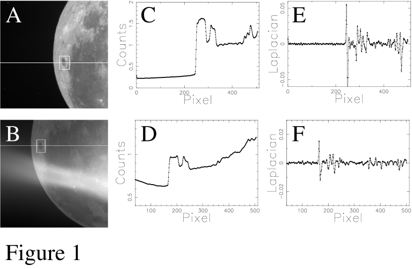
Figure 1: Example earthshine obserations. Panel A: An example of an earthshine image with no visible scattered light. Panel B: An example of a poor earthshine image with significant visible scattered light from telescope optics. Panels C,D: Flux along a section through earthshine image, as indicated by the white line in panels A and B. Panels E,F: Laplacian of image along same line. The maximum peaks correspond to the edge of the Moon.

Through a series of observations of the waxing crescent phase of the Moon in Cousins I and R filters (centered on 600 nm and 800 nm, respectively), we monitored hourly variation in the reflectivity of Earth centered along segments of constant latitude that intercept the continental coast between the southern tip of Africa and the Middle East. For comparison, we also measured a light curve of the Moon as a waning crescent to observe constant specular reflection from the South Pacific Ocean (data set F2). Our observations are summarized in Table 1 and are labeled as data sets C1–C5, F1–F2. The earthshine light curves, normalized by the intensity of the initial observation, are also presented along with the weather conditions for the corresponding reflecting region of Earth’s surface in Figure 2. Observations were made from a site near Romsey, 100 km north of metropolitan Melbourne, Australia $(37^{o}23^{\prime}$ S $144^{o}41^{\prime}$ E), with use of an $8"$ Meade Schmidt-Cassegrain telescope as a mount for a $512\times 512$ pixel charge-coupled device camera. The field of view is $20.8^{\prime}\times 20.8^{\prime}$. Images of the sunlit lunar crescent were taken contemporaneously with earthshine images to calibrate for changing air mass. The same two regions of the Moon (defined by lunar coordinates) were used to measure the moonshine and earthshine fluxes for a set of observations on a single night. Those earthshine regions for a waxing crescent are shown in Figure 1 (panels A and B) and are marked by the boxes. Use of the same regions within a night allows comparison of results, while limiting the systematic variations associated with the relative reflectivity of different regions of the Moon. When possible, the same region of the Moon was used for all sets of observation.. The time variation in absorption of flux was calculated by fitting the crescent intensity with Beer’s law of atmospheric extinction. The statistical uncertainty among crescent light curve points does not fully account for the level of departure of the data from the best fit. We therefore introduced an additional scatter (which might describe the presence of fluctuations in atmospheric opacity around the smooth trend) at a level such that the best-fit Beer’s Law has a reduced $\chi^{2}$ of unity. The earthshine light curve was divided by the estimate of Beer’s law, which yielded the relative change in intrinsic earthshine flux.

Light from the bright crescent flares into view of the charge-coupled device during earthshine exposures. This is particularly evident during large lunar phases and is a known difficulty in the data reduction for earthshine observations due to the telescope optics in imaging the dim earthshine region adjacent to the bright crescent. Previous studies have removed it by subtraction of a linear extrapolation of the background, which decreases radially from the center of the Moon (Qui et al., 2003; Arnold, 2007). In this work, we introduced a new technique to remove the scattered light. The scattered light has low spatial curvature when compared to the sharp lunar features (see Figure 1, panel B). After smoothing all images from a night of observation on a scale that corresponds to the seeing of the worst image (Gaussian across 6 pixels), we take the pixel-to-pixel Laplacian of the earthshine flux in a region with a highly variable surface, such as a crater. In this region, the scattered light is approximated as linearly changing with position. Figure 1 shows examples of images with minimal and significant visible scattered light (panels C, D respectively). The right hand panels show the corresponding Laplacian along a line through the variable region of the Moon (panels E, F).

Inspection of the Laplacian as a function of position reveals fluctuations about zero across the entire observed area. The size of these fluctuations is largest at positions coinciding with lunar surface features, and smallest in the area that corresponds to the sky. The utility of the method is demonstrated by panels B and F, which correspond to a particularly poor observation included here to demonstrate that scattered light removal via the described Laplacian technique is viable even in extreme cases. The Laplacian technique leaves residuals about zero in regions of the sky, underneath the prominent region of scattered light, that are as small as for the quality of image in panel A.

From the fact that the Laplacian has no trend to increase or decrease away from minimal variation about zero in regions of significant scattered light, as well as those with minimal scattered light, we conclude that there is no residual contribution of scattered light to the Laplacian.

On the other hand, features like craters show up as characteristic double horned profiles. The amplitudes of these features are proportional to the earthshine flux. An important advantage of this technique, which is designed specifically for our data analysis, is that it requires no prior knowledge of the distribution of background scattered light and is computationally simple. We base our light curve measurement on the maximum change in the Laplacian within a finite region. By choosing a finite region (shown as the box in Figure 1, panels A, B) rather than a point, we allow for error in image alignment. The regions are chosen to be the same for each night of observations, but as different data sets are not quantitatively compared via flux magnitude, an exact measure of the scattered light is not required. This also removes the need to quantify any change between nights in physical scale of the region over which the Laplacian is taken. The earthshine region used in sets C1–C5 and F1 is based on the Grimaldi crater. In set F2 it is based on Mare Crisium.

Results

In Figure 2, we show the results of our earthshine observations. The upper left panel (panel A) is a map of the Earth with lines showing the path taken by the central region of reflectance during each night of observation. For each night of observation, three panels are shown. The upper panel shows the color variation with time, the central panel shows the light curve, and the lower panel shows the central reflecting region for the observation with local weather information. In sets C1–C5, we attribute the decrease in earthshine flux of $10-20\%$ to the interruption of specular reflection from the Indian Ocean by the African coast rotating into view. In comparison, the light curves in sets F1 and F2 show little variation, with decreases of around $2\%$. This quiescence is due to the constant reflective properties of the diffusive desert regions of northern Africa (F1) and the constant specular reflection of the South Pacific Ocean (F2).

For data sets C1–C5, there is variation in the decrease per hour measured due to the differing local cloud cover, the latitude of the central reflection (due to the time of year), and the length of time for which the data is available. Data set C3 does not extend as far west, and hence, specular reflection would not have been totally interrupted. The remaining contribution to reflection by the Indian Ocean at later times will depend on the wave distribution off the coast (Williams and Gaidos, 2008). For data set C5, large local cloud formations are present over the ocean; this type of cloud cover will diffuse incident sunlight on the ocean and prevent specular reflection.

Discussion

To investigate the light curve trends quantitatively, we used a linear function to parameterize the variation of earthshine intensity with time. This function has the form: $I(t)=\alpha t+\beta$, where the parameters $\alpha$ and $\beta$ correspond to the gradient and intercept of a straight line for the intensity I(t), at time t, The rates of decrease $[d(\Delta I/I(t_{0}))/dt$, where $\Delta I=\alpha(\Delta t)]$ for each data set are presented in Table 1. Uncertainties were determined from the projection of the ellipse for which $\chi^{2}$ equals the minimum $\chi^{2}$ plus 1. The data sets C1–C5 exhibit statistically significant decreases in earthshine for observations spanning the African coast. Smaller decreases are detected in sets C3 and C5 owing to oceanic cloud cover and a lack of reflection points centered over continental Africa. The data sets F1 and F2 exhibit small (consistent with zero) decreases in earthshine due to the constant surface characteristics. The short time scale of the observations suggests that the cloud formations in the Moon’s line of sight, and their overall contribution to the scattered light, will remain fairly stable. Results are compared within a night of observations; therefore, the weather conditions are most important when local cloud masks specular reflection in some oceanic regions, for example, in set C5. As seen in earthshine observations of the vegetation red edge, weather conditions dictate the strength of the signal seen (Montañés-Rodríguez et al., 2006). However, in future long-term observations of extrasolar planets with evident weather systems, the rotational period may still be discernible by folding light curves (Pallé et al., 2008). We require more data sets to determine whether there is any dependence of our result on the phase angle of the Moon. We are unable to observe the crescent Earth via earthshine and, therefore, cannot measure the predicted increase in specular reflection due to the grazing angle (Williams and Gaidos, 2008).

We note that the measured change in earthshine flux is not the result of hourly variations in lunar phase. The intensity of reflected sunlight increases by around $0.15\%$ per hour at the lunar phase of the observations (Qui et al., 2003). In addition, the increase in lunar phase angle also corresponds to an increase in path length through the atmosphere, which, for our observations, corresponds to around a $1\%$ per hour decrease in the intensity of earthshine. Thus, the residual decrease in earthshine due to the Earth’s phase as seen from the Moon is below $1\%$ during a typical night of observations.

In addition to variable flux, our observations indicate associated changes in color, which we interpret as being due to some combination of the vegetation red-edge (Seager et al., 2005; Hamdani et al., 2006) and the increased reflectivity of deserts into the infrared (which reddens the scattered light as it decreases in brightness) (upper sub-panels in Figure 2). The results of a linear parameterization are presented in Table 1, where statistically significant reddening of the spectrum is measured for data sets C1, C2, and C4. This effect is not seen in set F2, where the reflecting surface is uniformly ocean. Moreover, there is a strong correlation between the decline in flux and color change for each data set (Figure 3). Thus, observation of a coast line crossing in reflected light from an extrasolar planet may be characterized not only by a sharp decline of flux, but also by reddening of the reflected spectrum. These ideas are supported by modeling by Stam (2008), where a cloudless planet shows more variation in the flux and polarization in the near infrared (0.87 $\mu m$) than toward the blue (0.44 $\mu m$) due to areas of vegetation compared to oceanic regions. For a realistic cloudy Earth model, the effect is decreased, as seen in earthshine observations of the vegetation red edge (Arnold, 2007). Further observations of other coast lines and land masses are required to determine whether the reddening of the spectrum is unique to our observations of Africa or whether they may be used in characterizing extrasolar planets as having continents and liquid oceans

Conclusions

The consistent decrease in earthshine flux in repeated observations corresponding to reflection from the African coast supports the idea that photometric variability may be used by future space-based missions to characterize terrestrial extrasolar planets, particularly those that have significant fractions of their surfaces covered by both seas and land masses. For example, surface features could be used to determine the rotational period of Earth-like planets (Pallé et al., 2008). We find the observed photometric variability associated with a continental coast crossing to be substantially larger than the measured spectral change due to vegetation’s red edge (Arnold, 2007). In addition, unlike the photometric properties of land and water, the spectral signature of vegetation might not be universal (Seager et al., 2003). Finally, variability is measured in broad bands rather than spectra, which makes this terrestrial signature more readily detectable. Further observations of the African coast and other landmasses will help determine the detectability of a coast via the reddening of the spectrum. Determining the phase dependence of the magnitude of the decrease, and more detailed analysis of the effect of weather on Earth’s variability, will require more observations. Spectropolarimetric modeling studies have suggested that the combination of photometric flux and polarization will yield the best characterization of surface types, therefore, further earthshine observations are justified (Williams and Gaidos, 2008).

Our results highlight the importance of considering specular reflection from oceans in the modeling and analysis of light curves from Earth-like extrasolar planets, and suggest that it is a useful tool in determining the presence of liquid water on a planet. Increasingly sophisticated modeling studies of photometric variability (Pallé et al., 2008; Williams and Gaidos, 2008), which account for the effects of viewing geometry, dynamic weather, and data quality on light curve characterization (Ford et al., 2001), are therefore justified by empirical studies of the Earth as a model extrasolar planet.

Acknowledgments:
We thank the anonymous referees for their detailed comments that enabled us to improve the clarity of the paper. This work was supported in part by grants from the Australian Research Council. SVL acknowledges the support of an Australian Postgraduate Award and a Postgraduate Overseas Research Experience Scholarship.

Author Disclosure Statement:
No competing financial interests exist.

Abreviation:
TPF, Terrestrial Planet Finder.

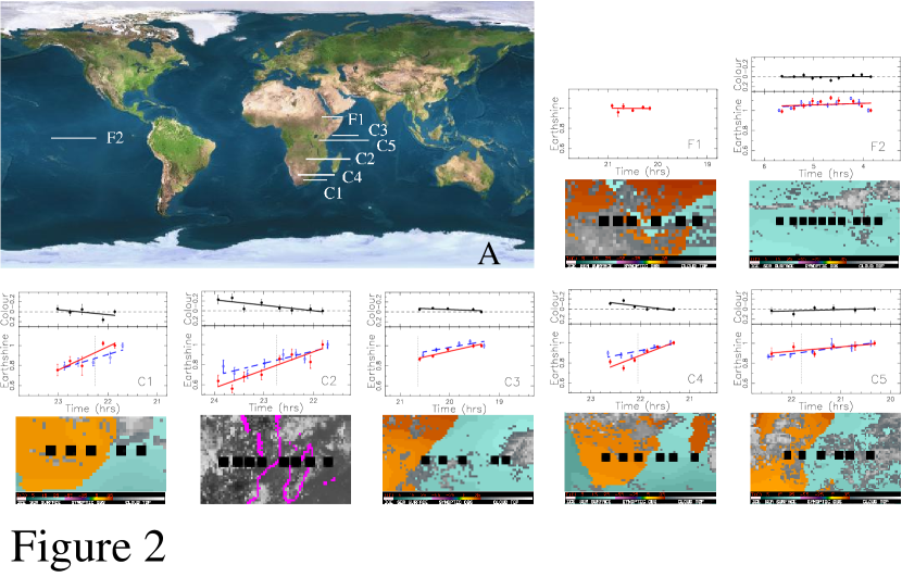
Figure 2: Earthshine light curves. Panel A shows the path of the central point of scattered light (Earth and Moon Viewer; see http://www.fourmilab.ch/earthview/vplanet.html.). The remaining panels (F1, F2, C1, C2, C3, C4 and C5) show: Middle sub-panel: Light curves for the Cousins $R$ (red) and $I$ (blue) filters, with the coastal crossing time (dotted). The smaller error bars show the statistical errors in photometry, the larger error bars include the intrinsic scatter in airmass around Beer’s law. Top sub-panel: Color change ($R-I$) with the corresponding linear fit (solid). Bottom sub-panel: Weather details for the region of reflected light with black boxes representing the center of reflection.

Figure 3: Correlation of flux change and color change. The magnitude of color change per hour for data sets C1–C5 and F2 are plotted versus the size of the decline in earthshine per hour in the R filter (solid). Error bars are quoted as 1$\sigma$ throughout this Paper.

Set	Date	Phase	Filter	Time $\Delta t$	$\chi^{2}_{R}$	$d(\Delta I/I_{0})/dt$	$d(I-R)/dt$
C1	12/04/05	8% waxing	I	1.18 hrs	1.74	-15.71$\pm^{7.82}_{2.43}$ %	-0.10$\pm^{0.13}_{0.03}$ %
			R	1.16 hrs	3.15	-22.62$\pm^{6.08}_{9.66}$ %
C2	01/05/06	31% waxing	I	2.11 hrs	0.99	-12.54$\pm^{2.99}_{1.82}$ %	-0.11$\pm^{0.05}_{0.03}$ %
			R	2.11 hrs	1.76	-18.56$\pm^{4.42}_{1.01}$ %
C3	08/28/06	16% waxing	I	1.23 hrs	2.52	-8.28$\pm^{2.73}_{1.77}$ %	-0.04$\pm^{0.02}_{0.03}$ %
			R	1.25 hrs	2.37	-10.94$\pm^{1.26}_{1.93}$ %
C4	11/24/06	10% waxing	I	1.26 hrs	3.52	-10.10$\pm^{3.09}_{1.17}$ %	-0.12$\pm^{0.04}_{0.03}$ %
			R	1.28 hrs	4.91	-19.02$\pm^{2.58}_{1.30}$ %
C5	08/19/07	32% waxing	I	2.07 hrs	0.47	-6.61$\pm^{1.46}_{1.97}$ %	0.03$\pm^{0.03}_{0.04}$ %
			R	2.08 hrs	1.04	-4.38$\pm^{2.89}_{1.56}$ %
F1	07/29/06	14% waxing	I	-	-	-	-
			R	0.76 hrs	1.78	0.0003$\pm^{0.002}_{0.006}$%
F2	04/14/07	16% waning	I	1.80 hrs	6.1	-1.88$\pm^{3.08}_{0.25}$ %	0.001$\pm^{0.004}_{0.014}$ %
			R	1.79 hrs	6.17	-2.21$\pm^{1.04}_{1.28}$ %

Table 1: Observational log and results from analysis of a linear fit to light curves. The quantity $\chi^{2}_{R}$ is the reduced $\chi^{2}$ value of the fit with scatter around Beer’s law. The percentage decrease is the decrease in earthshine intensity per hour for the linear fit. The far right column is the magnitude of the color change.

References

- (1) Arnold, L. (2007) Earthshine observation of vegetation and implication for life detection on other planets. Space Sci. Rev. doi: 10.1007/s11214–007–9281–4.
- (2) Des Marais, D.J., Harwit, M., Jucks, K., Kasting, J.F., Lunine, J.I., Lin, D., Seager, S., Schneider, J., Traub, W. and Woolf, N. (2001) Biosignatures and planetary properties to be investigated by the TPF mission. JPL Publication 01–008, Jet Propulsion laboratory, Pasedena, CA. Available online at .
- (3) Des Marais D.J., Harwit, M.O., Jucks, K.W., Kasting, J.F., Lin, D.N.C., Lunini, J.I., Schneider, J., Seager, S., Traub, W.A. and Woolf, N.J. (2002) Remote sensing of planetary properties and biosignatures on extrasolar terrestrial planets. Astrobiology 2:153–181.
- (4) Ford, E.B., Seager, S. and Turner, E.L. (2001) Characterization of extrasolar terrestrial planets from diurnal photometric variability. Nature 412:885–887.
- (5) Goode, P.R., Qui, J., Yurchyshyn, V., Hickey, J., Chu, M.-C., Kolbe, E., Brown, C.T. and Koonin, S.E. (2001) Earthshine observations of the Earth’s reflectance. Geophys. Res. Lett. 28:1671–1674.
- (6) Hamdani, S., Arnold, L., Foellmi, C., Berthier, J., Billeres, M., Briot, D., François, P., Riaud, P. and Schneider, J. (2006) Biomarkers in disk-averaged near-UV to near-IR Earth spectra using Earthshine observations. Astron. Astrophys. 460:617–624.
- (7) Howard, A. and Horowitz, P. (2001) Optical SETI with NASA’s Terrestrial Planet Finder. Icarus 150:163–167.
- (8) McCullough, P.R. (2006) Models of polarized light from oceans and atmospheres of Earth-like extrasolar planets. arXiv: astro-ph/0610518v1.
- (9) Montañés-Rodríguez, P., Pallé, E., Goode, P.R., Hickey, J. and Koonin, S.E. (2005) Globally integrated measurements of the Earth’s visible spectral albedo. Astrphys. J. 62:1175–1182.
- (10) Montañés-Rodríguez, P., Pallé, E., Goode, P.R. and Martín-Torres, F.L. (2006) Vegetation signature in the observed globally integrated spectrum of Earth considering simultaneous cloud data: Applications for extrasolar planets. Astrphys. J. 651:544–552.
- (11) Montañés-Rodríguez, P., Pallé, E. and Goode, P.R. (2007) Measurements of the surface brightness of the earthshine with applications to calibrate lunar flashes. Astron. J. 134:1145–1149.
- (12) Pallé, E., Goode, P.R., Yurchyshyn, V., Qui, J., Hickey, J., Montañés-Rodríguez, P., Chu, M.-C., Kolbe, E., Brown, C.T. and Koonin, S.E. (2003) Earthshine and the Earth’s albedo: 2. Observations and simulations over 3 years. J. Geophys. Res. 108, doi:10.1029/2003JD003611..
- (13) Pallé, E., Ford, E.B., Seager, S., Montañés-Rodríguez, P. and Vazquez, M. (2008) Identifying the rotation rate and the presence of dynamic weather on extrasolar Earth-like planets from photometric observations. Astrophys. J. 676:1319–1329.
- (14) Qui, J., Goode, P.R., Pallé, E., Yurchyshyn, V., Hickey, J., Montañés-Rodríguez, P., Chu, M.-C., Kolbe, E., Brown, C.T. and Koonin, S.E. (2003) Earthshine and the Earth’s albedo: 1. Earthshine observations and measurements of the lunar phase function for accurate measurements of the Earth’s Bond albedo. J. Geophys. Res. 108, doi:10.1029/2003JD003610.
- (15) Sagan, C., Thompson, W.R., Carlson, R., Gurnett, D. and Hord, C. (1993) A search for life on Earth from the Galileo spacecraft. Nature 365:715–721.
- (16) Seager, S. (2003) The search for extrasolar Earth-like planets. Earth Planet Sci. Lett. 208:113–124.
- (17) Seager, S., Ford, E.B. and Turner, E.L. (2003) Characterizing Earth-like planets with terrestrial planet finder. Proceedings of SPIE 4835:79–86.
- (18) Seager, S., Turner, E.L., Schafer, J. and Ford, E.B. (2005) Vegetation’s Red Edge: A possible spectroscopic biosignature of extraterrestrial plants. Astrobiology 5:372–390.
- (19) Sotin, C. (2007) Titan’s lost seas found. Nature 445:29–30.
- (20) Stam, D.M. (2008) Spectropolarimetric signatures of Earth-like extrasolar planets. Astron. Astrophys. 482:989-1007.
- (21) Stofan, E.R., Elachi, C., Lunine, J.I., Lorenz, R.D., Stiles, B., Mitchell, K.L., Ostro, S., Soderblom., L., Wood, C., Zebker, H., Wall, S., Janssen, M., Kirk, R., Lopes, R., Paganelli, F., Radebaugh, J., Wye, L., Anderson, Y., Allison, M., Boehmer, R., Callahan, P., Encrenaz, P., Flamini, E., Francescetti, G., Gim, Y., Hamilton, G., Hensley, S., Hojnson, W.T.K., Kelleher, K., Muhleman, D., Paillou, P., Picardi, G., Posa, F., Roth, L., Seu, R., Shaffer, S., Vetrella, S., and West, R. (2007) The lakes of Titan. Nature 445:61–64.
- (22) Tinetti, G., Meadows, V.S., Crisp, D., Kiang, N.Y., Kahn, B.H., Bosc, E., Fishbein, E., Velusamy, T. and Turnbull, M. (2006) Detectability of planetary characteristics in disk-averaged spectra II: Synthetic spectra and light-curves of Earth. Astrobiology 6:881–900.
- (23) Turnbull, M.C., Traub, W.A., Jucks, K.W., Woolf, N.J., Meyer, M.R., Gorlova, N., Skrutskie, M.F. and Wilson, J.C. (2006) Spectrum of a habitable world: Earthshine in the near-infrared. Astrophys. J. 644:551–559.
- (24) Williams, D.M. and Gaidos, E. (2008) Detecting the glint of starlight on the oceans of distant planets. Icarus 195:927–937.
- (25) West, R.A., Brown, M.E., Salinas, S.V., Bouchez, A.H., and Roe, H.G. (2005) No oceans on Titan from the absence of near-infrared specular reflection. Nature 436:670–672.
- (26) Woolf, N.J., Smith,P.S., Traub, W.A. and Jucks, K.W. (2002) The spectrum of Earthshine: A pale blue dot observed from the ground. Astrphys. J. 574:430–433.