Lagrangian studies in convective turbulence

Abstract

We present high-resolution direct numerical simulations of turbulent three-dimensional Rayleigh-Bénard convection with a focus on the Lagrangian properties of the flow. The volume is a Cartesian slab with an aspect ratio of four bounded by free-slip planes at the top and bottom and with periodic side walls. The turbulence is inhomogeneous with respect to the vertical direction. This manifests in different lateral and vertical two-particle dispersion and in a dependence of the dispersion on the initial tracer position for short and intermediate times. Similar to homogeneous isotropic turbulence, the dispersion properties depend in addition on the initial pair separation and yield a short-range Richardson-like scaling regime of two-particle dispersion for initial separations close to the Kolmogorov dissipation length. The Richardson constant is about half the value of homogeneous isotropic turbulence. The multiparticle statistics is very close to the homogeneous isotropic case. Clusters of four Lagrangian tracers show a clear trend to form flat, almost coplanar objects in the long-time limit and deviate from the Gaussian prediction. Significant efforts have been taken to resolve the statistics of the acceleration components up to order four correctly. We find that the vertical acceleration is less intermittent than the lateral one. The joint statistics of the vertical acceleration with the local convective and conductive heat flux suggests that rising and falling thermal plumes are not associated with the largest acceleration magnitudes. It turns out also that the Nusselt number which is calculated in the Lagrangian frame converges slowly in time to the standard Eulerian one.

I Introduction

Turbulent convection is one of the best studied fundamental flows in fluid dynamics research Kadanoff2001 ; Ahlers2009 . One reason is the large range of examples and applications in nature and technology for which a turbulent motion is initiated and sustained by heating a fluid from below and cooling from above. Almost all of these studies have been conducted in the Eulerian frame of reference. They were primarily focussed to the mechanisms of local Shishkina2007 ; Zhou2007 ; Shishkina2008 ; Emran2008 and global Kerr1996 ; Niemela2000 ; Amati2005 ; Funfschilling2005 turbulent heat transfer.

The Lagrangian perspective of turbulence, in which the fields are monitored along the trajectories of infinitesimal fluid parcels, has recently produced new insights into the local topology of fluid parcel tracks, the local strength of accelerations, and the statistics of time increments of turbulent fields Toschi2009 ; Schumacher2009 . The progress is caused on the one hand by significant innovations in the experimental techniques, such as three-dimensional particle tracking Mann2000 ; LaPorta2001 ; Guala2005 or acoustic methods Mordant2001 . On the other hand, direct numerical simulations of turbulence become now feasible that resolve three-dimensional Lagrangian turbulence at moderate and higher Reynolds numbers Yeung2002 ; Boffetta2002 ; Biferale2005 ; Sawford2008 . Both, experiments and simulations, made a deeper understanding of the small-scale intermittency and its connection with large accelerations of fluid parcels possible.

Lagrangian investigations in convective turbulence are however rare. Several reasons can be given for this circumstance. First, on the experimental side it is desirable to monitor the temperature along the particle tracks beside the velocity components and the accelerations. Only recently, Gasteuil et al. Gasteuil2007 constructed therefore a smart particle, that monitors velocity, temperature and orientation while moving through the cell. Due to the integrated power supply the particle diameter remained however larger than the thermal boundary layer thickness, such that the large-scale bulk motion can be monitored only. Second, it is also clear that the complexity of direct numerical simulations increases since the temperature field has to be advected in addition to the velocity. Temperature tracking along the tracer positions requires additional interpolations. Furthermore, one cannot return to simulations in a fully periodic cube, the so-called homogeneous Rayleigh-Bénard convection setup, since the periodicity in the direction of the mean temperature gradient causes a self-amplifying fluid motion. This was discussed in detail by Calzavarini et al. Calzavarini2005 ; Calzavarini2006 . Third, the turbulence is inhomogeneous –at least in the vertical direction as in the following setup– and it is thus not clear which of findings from the homogeneous isotropic purely hydrodynamic turbulence pertain. For example, the height dependence of the statistics has to be considered additionally.

First numerical attempts have been made recently to study some aspects of the heat transfer and tracer dispersion in the Lagrangian framework of convective turbulence Schumacher2008 . The motivation of the study can be condensed in one question: Which new insight into the nature of turbulent convection provides the complementary Lagrangian view? One result of Schumacher2008 was to determine a mixing zone which is dominated by rising and falling thermal plumes. This is done by combining acceleration and local convective heat flux statistics. The mixing zone starts right above the thermal boundary layer and extends several tens of the boundary layer thickness into the bulk of the cell. Thermal plumes are fragments of the thermal boundary layer that detach in the vicinity of the top and bottom isothermal planes. The existence of a mixing zone has been suggested in several Eulerian studies on the basis of other criteria, e.g. Castaing1989 ; Xia2002 and was thus confirmed in the complementary Lagrangian frame of reference Schumacher2008 .

The present work extends the previous study Schumacher2008 into several directions. Beside the local convective, the local conductive heat flux is studied along the tracer tracks. It requires to monitor temperature gradient components. Furthermore, the analysis of the Lagrangian tracer dispersion is extended. In addition to the hydrodynamic case Sawford2008 , we study the dependence of pair dispersion on the initial separation and the initial seeding position. As discussed in Refs. Chertkov1999 ; Pumir2000 ; Biferale2005 for the pure hydrodynamic case, higher order particle statistics requires to track little clusters of tracers. We provide here an analysis of the four-particle-statistics, where the tracers start out of groups of tetrahedra of different sidelengths and initial vertical positions.

The outline of the manuscript is as follows. In the next section the equations of motion, the numerical scheme, the Lagrangian tracer tracking and the turbulent heat transfer. In section III, some results of the Eulerian statistics of the temperature field are presented. This section is followed by sections on the Lagrangian particle dispersion, the acceleration statistics and the conductive and convective heat flux. We conclude with a short discussion of our results and will give a brief outlook to possible extensions of the present work.

II Numerical model

II.1 Equations of motion and boundary conditions

The Boussinesq equations, i.e. the Navier-Stokes equations for an incompressible flow with an additional buoyancy term $\alpha g\theta{\bm{e}}_{z}$ and the advection-diffusion equation for the temperature field, are solved by a standard pseudospectral method for the three-dimensional case Schumacher2007 . The equations are given by

$${\bm{\nabla}\cdot\bm{u}} = 0\,,$$ (1)

$$\frac{\partial{\bm{u}}}{\partial t}+({\bm{u}\cdot\bm{\nabla}}){\bm{u}} = -{\bm{\nabla}}p+\nu{\bm{\nabla}}^{2}{\bm{u}}+\alpha g\theta{\bm{e}}_{z}\,,$$ (2)

$$\frac{\partial\theta}{\partial t}+({\bm{u}\cdot\bm{\nabla}})\theta = \kappa{\bm{\nabla}}^{2}\theta+u_{z}\frac{\Delta T}{H}\,.$$ (3)

Here, ${\bm{u}}$ is the turbulent velocity field, $p$ the (kinematic) pressure field and $\theta$ the temperature fluctuation field. The system parameters are: gravity acceleration $g$, kinematic viscosity $\nu$, thermal diffusivity $\kappa$, vertical temperature gradient $\Delta T/H$, and thermal expansion coefficient $\alpha$. The temperature field is decomposed into a linear profile and fluctuations $\theta$ about the profile

$$T({\bm{x}},t)=-\frac{\Delta T}{H}(z-H/2)+\theta({\bm{x}},t)\,.$$ (4)

Since $T$ is prescribed and constant at bottom and top boundaries $z=0$ and $z=H$, the condition $\theta=0$ follows there. Here, $\Delta T>0$. The dimensionless control parameters are the Prandtl number $Pr$, the Rayleigh number $Ra$, and the aspect ratio $\Gamma$,

$$Pr = \frac{\nu}{\kappa}\,,$$ (5)

$$Ra = \frac{\alpha gH^{3}\Delta T}{\nu\kappa}\,,$$ (6)

$$\Gamma = \frac{L}{H}\,.$$ (7)

The simulation domain is $V=L\times L\times H=[0,\Gamma\pi]\times[0,\Gamma\pi]\times[0,\pi]$. In lateral directions $x$ and $y$, periodic boundary conditions are taken. In the vertical direction $z$, free-slip boundary conditions are used which are given by

$$u_{z}=\theta=0\;\;\;\;\mbox{and}\;\;\;\;\partial_{z}u_{x}=\partial_{z}u_{y}=0\,.$$ (8)

The computational grid has a size of $N_{x}\times N_{y}\times N_{z}=2048\times 2048\times 513$ points. For an aspect ratio $\Gamma=4$, it is thus equidistant in all three space directions with a grid spacing $\Delta x$. Time-stepping is done by a second-order predictor-corrector scheme. The production runs are conducted on one rack of the Blue Gene/P system which corresponds with 4096 MPI tasks Schumacher2007 . We use volumetric Fast Fourier Transforms based on the p3dfft package by D. Pekurovsky Pekurovsky2008 . The spectral resolution is $k_{max}\eta_{K}=4.5$ where $k_{max}=2\sqrt{2}\pi N_{x}/(3L_{x})$. Quantity $\eta_{K}=\nu^{3/4}/\langle\epsilon\rangle^{1/4}$ is the Kolmogorov scale with the mean energy dissipation rate $\langle\epsilon\rangle$.

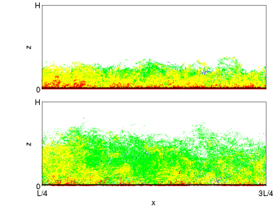
Figure 1: (Color online) Side view of two instantaneous Lagrangian tracer distributions at $t=9.5\tau_{\eta}$ (top) and $t=19\tau_{\eta}$ (bottom). The tracers are colored with respect to the local temperature $T$ at their position. Four intervals are taken: $T\in[\Delta T/2,\Delta T/3]$, $T\in[\Delta T/3,\Delta T/6]$, $T\in[\Delta T/6,0]$ and for $T\in[0,-\Delta T/6]$. The whole ensemble consists of $2\times 10^{5}$ tracers. Tracers started in the whole $x-y$ plane at the height of the thermal boundary layer thickness which is indicated by the solid line very close to the bottom plane in both plots.

II.2 Lagrangian particle tracking

Lagrangian tracer particles follow the streamlines of the turbulent velocity field in correspondance with

$$\dot{\bm{x}}={\bm{u}}({\bm{x}}(t),t)\,.$$ (9)

For the majority of the analysis, we seeded $3\times 10^{5}$ tetrahedra aligned along the outer coordinate axes in the box, i.e. ${\bm{x}}_{1}={\bm{x}}_{0}$, ${\bm{x}}_{2}={\bm{x}}_{0}+{\ell}{\bm{e}}_{x}$, ${\bm{x}}_{3}={\bm{x}}_{0}+{\ell}{\bm{e}}_{y}$, and ${\bm{x}}_{4}={\bm{x}}_{0}+{\ell}{\bm{e}}_{z}$. The vector ${\bm{x}}_{0}$ is randomly chosen in the box. The tracer ensemble was divided into 6 six groups with initial sidelengths of ${\ell}=1,2,4,8,16$ and 32 grid spacings $\Delta x$ which correspond with 0.5, 1, 2, 4, 8 and 16 $\eta_{K}$. The two-particle dispersion analysis is consequently conducted for the three tracer pairs $\{{\bm{x}}_{1},{\bm{x}}_{2}\}$, $\{{\bm{x}}_{1},{\bm{x}}_{3}\}$, and $\{{\bm{x}}_{1},{\bm{x}}_{4}\}$ of each tetrahedron.

For the two- and multiparticle statistics, we run in addition a simulation with the following initial conditions: again ${\bm{x}}_{1}={\bm{x}}_{0}$, ${\bm{x}}_{2}={\bm{x}}_{0}+{\ell}{\bm{e}}_{x}$, ${\bm{x}}_{3}={\bm{x}}_{0}+{\ell}{\bm{e}}_{y}$, and ${\bm{x}}_{4}={\bm{x}}_{0}+{\ell}{\bm{e}}_{z}$. The $x$ and $y$ coordinates of the vector ${\bm{x}}_{0}$ are again randomly chosen. The vertical coordinate corresponds with $z_{0}=\delta_{T}/2$, $\delta_{T}$, $10\delta_{T}$, $20\delta_{T}$ and $H/2$. Here, we pick ${\ell}=\eta_{K}/2$ and $2\eta_{K}$.

The Lagrangian particles are advanced in time simultaneously with the Boussinesq equations. The velocity, temperature and temperature gradient components at intergrid positions are calculated by trilinear interpolation. The full particle set is written out each 0.45 $\tau_{\eta}$. Here, $\tau_{\eta}=\sqrt{\nu/\langle\epsilon\rangle}$ is the Kolmogorov time. Accelerations along the Lagrangian tracks are calculated from three successive integration steps ($\Delta t=0.006\tau_{\eta}$) and the output interval is the same as for the particle positions, velocities, temperature, and temperature gradient. We thus gather Lagrangian statistics over up to $4.8\times 10^{8}$ tracer particle events. Figure 1 illustrates the initial phase of the tracer dispersion. All tracers start from a $x-y$ plane close to the bottom wall.

II.3 Turbulent heat transfer

The convective turbulence is studied for one parameter setting. The Rayleigh number is $Ra=1.2\times 10^{8}$, the Prandtl number $Pr=0.7$ and the aspect ratio $\Gamma=4$. The response of the system is a turbulent heat transport as quantified by the dimensionless (Eulerian) Nusselt number which is given for a plane at fixed height $z$ by

$$Nu(z)=\frac{\langle u_{z}T\rangle_{A,t}-\kappa\partial_{z}\langle T\rangle_{A,t}}{\kappa\Delta T/H}\,,$$ (10)

where $\langle\cdot\rangle_{A,t}$ denote averages in planes at $z$ and with respect to time. The value of $Nu(z)$ is constant and independent of $z$. The global Nusselt number is then defined as

$$Nu=\frac{1}{H}\int_{0}^{H}Nu(z)\mbox{d}z=1+\frac{H}{\kappa\Delta T}\langle u_{z}T\rangle_{V,t}\,,$$ (11)

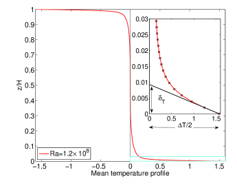
Figure 2: (Color online) Mean temperature profile $\langle T(z)\rangle_{A,t}$ of the turbulent convection run at $Ra=1.2\times 10^{8}$ and $Pr=0.7$. The inset shows the resolution of the thermal boundary layer with 7 grid planes. It also indicates the geometric interpretation of the thermal boundary layer thickness $\delta_{T}$ (see the text). The lower right box in the main figure indicates the size of the magnification.

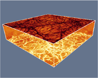
Figure 3: (Color online) Contour plot of the instantaneous temperature field $T({\bm{x}},t_{0})$.

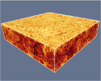
Figure 4: (Color online) Contour plot of the instantaneous thermal dissipation rate field $\chi({\bm{x}},t_{0})$. Data correspond to those in Fig. 3. In order to highlight the small-amplitude dissipation filaments in the bulk, we plot contours of the decadic logarithm of $\chi$.

where $\langle\cdot\rangle_{V,t}$ is a combined volume and time average. The Nusselt number for the present free-slip boundary case follows to $Nu=56.36\pm 0.59$. Similar to Julien et al. Julien1996 , we find an enhanced turbulent heat transport in comparison to no-slip top and bottom plates. For Rayleigh numbers between $9.8\times 10^{5}$ and $1.2\times 10^{8}$, we fit the power law $Nu=0.166\times Ra^{0.316}$ to the data.

III Eulerian temperature statistics

Figure 2 displays the mean temperature profile as a function of height. The total temperature can take values between $-\Delta T/2$ and $\Delta T/2$ only. As typical for higher Rayleigh numbers, the jump of mean profile to zero is observed across a thin layer, the thermal boundary layer. The inset magnifies the vicinity of the bottom plate. The thickness of the thermal boundary layer is defined as

$$\delta_{T}=\frac{H}{2Nu}\,.$$ (12)

For $z=0$, the conductive part of (10) contributes to $Nu$ only and we can set $Nu=-\kappa\partial_{z}\langle T\rangle_{A,t}|_{z=0}/(\kappa\Delta T/H)$. This leads to $\delta_{T}=-\Delta T/(2\partial_{z}\langle T\rangle_{A,t}|_{z=0})$ and to the geometric derivation of the thermal boundary layer thickness (as indicated in the inset of Fig. 2). In contrast to the no-slip case, we have $\langle u_{x}\rangle_{A,t}=\langle u_{y}\rangle_{A,t}=\langle u_{z}\rangle_{A,t}=0$ . Consequently, no velocity boundary layer is present. The Taylor microscale Reynolds number $R_{\lambda}=\sqrt{5/(3\nu\langle\epsilon\rangle)}\,\langle u_{i}^{2}\rangle\approx 143$.

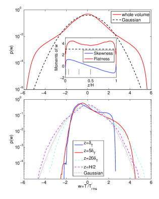
Figure 5: (Color online) Statistics of the temperature fluctuations $w=T^{\prime}/T^{\prime}_{rms}$. Top: Probability density function (PDF) of the temperature fluctuations. Data are compared with a Gaussian distribution (dashed line). Inset: Skewness and flatness of the temperature fluctuations $w$ as a function of the vertical coordinate $z/H$. The profiles are obtained by averaging over lateral planes and a sequence of statistically independent snapshots. The Gaussian value for the flatness $F=3$ is indicated by the dashed line. Bottom: PDFs of the temperature fluctuations taken in different planes which are indicated in the legend and by vertical solid lines in the inset of the top figure.

Figure 3 shows an instantaneous snapshot of the total temperature field $T({\bm{x}},t)$. Contour plots in two sideplanes and close to the top and bottom planes are shown. We observe a typical feature of thermal convection – the ridge-like maxima which correspond with thermal plumes that detach randomly. They form a skeleton which is advected by the flow close to the boundaries. The plumes coincide with local maxima of the thermal dissipation rate field (see Fig. 4 and compare it with Fig. 3) which is defined as

$$\chi({\bm{x}},t)=\kappa({\bm{\nabla}}T^{\prime}({\bm{x}},t))^{2}\,.$$ (13)

The definition contains the temperature fluctuations which are given by

$$T^{\prime}({\bm{x}},t)=T({\bm{x}},t)-\langle T(z)\rangle_{A,t}\,.$$ (14)

The probability density function (PDF) of $T^{\prime}$ is shown in Fig. 5. We compare the PDF of data taken from the whole slab volume with the Gaussian statistics in the top figure. Similar to findings for turbulent convection in closed cylindrical vessels with solid walls the temperature field statistics deviates from Gaussian Emran2008 . The analysis can be refined. The inset of the top panel shows therefore vertical profiles of the plane- and time-averaged flatness, $F=\langle T^{\prime\,4}\rangle_{A,t}/\langle T^{\prime\,2}\rangle_{A,t}^{2}$. The flatness differs clearly from the Gaussian value of 3 in all parts of the convection cell. In addition we plot the profile of the plane- and time-averaged skewness $S=\langle T^{\prime\,3}\rangle_{A,t}/\langle T^{\prime\,2}\rangle_{A,t}^{3/2}$ in the same inset. The magntiude of the skewness peaks at about $5\delta_{T}$ which is well inside the plume mixing zone Schumacher2008 . Both profiles agree also qualitatively with those by Kerr Kerr1996 and by Ref. Emran2008 which have been conducted with no-slip top and bottom boundaries. In the bottom panel of Fig. 5 we show the PDF of the temperature fluctuations in four different planes (see the legend). The PDF in the midplane comes closest to a Gaussian profile. Our data suggest that the free-slip boundary conditions lead to smaller deviations from Gaussianity compared to the no-slip case. It should also be noted that for strong rotation of the cell about the vertical coordinate the temperature fluctuations are Gaussian for both, no-slip and free-slip boundary conditions, as reported by Julien et al. Julien1996 .

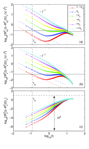
Figure 6: (Color online) Vertical and lateral particle pair dispersion as a function of the initial pair separation. (a) Compensated lateral dispersion for different initial separations as indicated in the legend. The dashed lines correspond with Eq. (18) for $R_{0}=\eta_{K}/2$ and $R_{0}=\eta_{K}$ and with Eq. (19) for $R_{0}=8\eta_{K}$ and $R_{0}=16\eta_{K}$. (b) Compensated vertical dispersion. Again, Eqs. (18) and (19) are fitted to the data for the same initial separations. (c) Same data as in (b) without compensation by $\langle\epsilon\rangle t^{3}$. The vertical dispersion is constrained between the planes and levels thus off at larger times. The square of the cell height, $H^{2}$, and the Kolmogorov time scale, $\tau_{\eta}$, are indicated. All axes are given in decadic logarithm. Tracer pairs are seeded initially across the whole volume.

IV Lagrangian particle dispersion

IV.1 Two-particle dispersion

The Eulerian framework analysis of turbulent convection demonstrated already that the flow is indeed inhomogeneous with respect to the vertical direction. Furthermore, we recall that the Lagrangian tracer motion is constrained between $z=0$ and $H$ since both walls cannot be penetrated. One motivation to study the dispersion in three-dimensional turbulent convection is therefore to verify if the classical Richardson dispersion law Richardson1926 can be also observed for the present case. Recall that the Richardson dispersion law follows from a solution of a diffusion problem which assumes a homogeneous and isotropic turbulent state. It states that, given two particle tracks, ${\bm{x}}_{2}(t)$ and ${\bm{x}}_{1}(t)$ with ${\bm{x}}_{i}=(x_{i},y_{i},z_{i})$, the distance vector ${\bm{R}}(t)={\bm{x}}_{2}(t)-{\bm{x}}_{1}(t)$ will follow

$$\langle R^{2}(t)\rangle_{L}=g_{3d}\langle\epsilon\rangle t^{3}\,,$$ (15)

where $g_{3d}$ is a universal constant of ${\cal O}(1)$. The symbol $\langle\cdot\rangle_{L}$ denotes an average over Lagrangian particle tracks. We decompose the relative tracer motion into a lateral and vertical contribution in order to separate homogeneous and inhomogeneous directions. The distance vector can be written as

$${\bm{R}}(t)={\bm{R}}_{xy}(t)+R_{z}(t){\bm{e}}_{z}.$$ (16)

The lateral two-particle dispersion is given by $\langle R^{2}_{xy}(t)-R^{2}_{xy}(0)\rangle_{L}$ where the average is taken over $6\times 10^{5}$ particle pairs. Here,

$${\bm{R}}_{xy}=[x_{2}(t)-x_{1}(t)]{\bm{e}}_{x}+[y_{2}(t)-y_{1}(t)]{\bm{e}}_{y}\,.$$ (17)

Similarly, the vertical dispersion is given by $\langle R^{2}_{z}(t)-R^{2}_{z}(0)\rangle_{L}$. The dispersion in each space direction would contribute with a weight of 1/3 in homogeneous isotropic turbulence. In order to compare our pair dispersion results with the predictions for isotropic turbulence, we will introduce two weight factors, $C_{xy}=2/3$ for the lateral motion and $C_{z}=1/3$ for the vertical one.

Figure 6 displays both dispersion processes with respect to time for six different initial pair separations as explained in section II C. The two-particle dispersion is given by a compensated plot in panels (a) and (b) of the figure. The graphs are normalized by $\langle\epsilon\rangle t^{3}$ to capture a Richardson-like scaling as a plateau. The initial ballistic behavior at small separations causes then an algebraic decay with $t^{-1}$. Following Sawford et al. Sawford2008 , we fit the following two relations to our data at small times

$$\frac{\langle R^{2}_{m}(t)-R^{2}(0)\rangle_{L}}{\langle\epsilon\rangle t^{3}}=\frac{C_{m}}{3}\left(\frac{R_{m}(0)}{\eta_{K}}\right)^{2}\frac{\tau_{\eta}}{t}$$ (18)

if $R_{m}(0)\ll\eta_{K}$ and

$$\frac{\langle R^{2}_{m}(t)-R^{2}_{m}(0)\rangle_{L}}{\langle\epsilon\rangle t^{3}}=\frac{11C_{m}}{3}C\left(\frac{R_{m}(0)}{\eta_{K}}\right)^{2/3}\frac{\tau_{\eta}}{t}$$ (19)

if $\eta_{K}\ll R_{m}(0)\ll L$. Here $L$ is the outer scale of turbulence and $C\approx 2$ Sawford2008 . Index $m$ stands for the lateral terms, $xy$, or the vertical term, $z$. The agreement with (18) for the initial Kolmogorov and sub-Kolmogorov separations is reasonable. For larger initial separations we use (19). The larger the initial separation the better agree prediction and data. We fitted the two smallest and largest initial separations only. None of the initial separations is neither much smaller nor much larger than the Kolmogorov scale which explains the slight deviations of the numerical results from the laws (18) and (19).

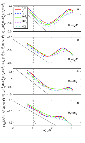
Figure 7: (Color online) Vertical and lateral particle pair dispersion as a function of the initial vertical seeding position $z_{0}$. (a) Compensated lateral dispersion for different initial heights $z_{0}$ as indicated in the legend (holds for all four figures). The initial tracer separation is $R_{0}=\eta_{K}/2$. (b) Compensated vertical dispersion. The initial separation is also $R_{0}=\eta_{K}/2$. (c) Compensated lateral dispersion. The initial separation is now $R_{0}=2\eta_{K}$. (d) Compensated vertical dispersion. Again $R_{0}=2\eta_{K}$. All axes are given in decadic logarithm and the Kolmogorov time scale is indicated by a dashed line. The solid line follows $\sim t^{-1}$ in all plots.

As discussed for example in Refs. Bourgoin2006 ; Sawford2008 , the establishment of a Richardson-like regime depends sensitively on the initial separation between the tracers. Indeed, for one of the six different separations the lateral dispersion curve passes through a small plateau with a Richardson constant $g_{xy}\approx 0.25$. This is observed for an initial separation of $R_{xy}(0)=2\eta_{K}$, (see solid line in Fig. 6(a)). The re-translation of the proportionality constant $g_{xy}$ into a three-dimensional homogeneous isotropic turbulence case is obtained by

$$\tilde{g}_{xy}=\frac{g_{xy}}{C_{xy}}=\frac{3}{2}g_{xy}\approx 0.375\,.$$ (20)

The proportionality constant is smaller than the value $g_{3d}\approx 0.5-0.6$ for homogeneous isotropic turbulence Boffetta2002 ; Biferale2005 ; Sawford2008 . In Ref. Schumacher2008 , it was already shown that the PDF of the lateral particle pair distance can be fitted to the stretched exponential form of Richardson Richardson1926 , however not to the Gaussian shape as suggested by Batchelor Batchelor1950 .

Figures 6(b) and (c) display the vertical dispersion. In panel (b), we repeat the compensated plot of panel (a) and show the fits to (18). A plateau is observed now for initial separations between $1\eta_{K}$ and $2\eta_{K}$. The resulting constant is $g_{z}\approx 0.05$ (see solid line in Fig. 6(b)). If one combines the lateral and vertical dispersion, the Richardson constant for the turbulent convection follows to

$$g_{xy}+g_{z}\approx 0.3\,,$$ (21)

which is less than our earlier estimate of $\tilde{g}_{xy}\approx 0.375$ and $g_{3d}\approx 0.5-0.6$. A smaller Richardson constant corresponds with a stronger correlated pair motion. Such behavior can be attributed to the presence of rising and falling thermal plumes - a feature that is absent in isotropic turbulence. Additionally, it is known that the plumes can cluster and form a large scale circulation Ahlers2009 . Figure 6(c) demonstrates that the vertical dispersion is constrained by the top and bottom planes. The vertical contribution $\langle R_{z}^{2}(t)-R^{2}_{z}(0)\rangle_{L}$ to the pair dispersion levels off. Eventually the lateral dispersion contributes solely to the long-time behavior.

The specifics of the present inhomogeneous flow is that not only the initial pair separation, but also the initial seeding position is important. This brings us to the second series of particle dispersion studies where tracer pairs with fixed distance in different horizontal planes of the slab are seeded (see section II C for details) and shorter simulations for about half the duration are rerun. Figure 7 summarizes our findings. We picked five intial seeding heights: two in the boundary layer, two in the plume mixing zone Schumacher2008 and the center plane. While panels (a) and (b) are for $R_{0}=\eta_{K}/2$, panels (c) and (d) are for $R_{0}=2\eta_{K}$. The latter is the separation that yielded a short Richardson-like range in Fig. 6(a).

Figures 7(a) and (c) show that the lateral dispersion curves of the tracer subgroups differ in magnitude. The local slope is however nearly the same for all subsets. The situation is slightly different for the vertical dispersion: while the seeding in the center plane causes a gradual variation of the local slope of the dispersion curve (see Figs. 7(b) and (d)), the seeding in the thermal boundary layer leads to significant differences after the initial ballistic period. The same result is observed in Fig. 7(d). The reason is that the tracer pairs probe then the detachment of the boundary layer fragments to full extent. This is not the case when starting in the bulk of the cell. It can also be observed that a plateau (which would imply Richardson-like scaling) depends sensitively on the intial separation and seeding height.

To summarize this part, Richardson-like dispersion appears for a very small range of scales in the present flow. Similar to previous studies, we confirm that the initial pair dispersion depends sensitively on both, the initial pair separation and the initial vertical position of a tracer pair in the volume. The qualitative behavior of the tracer dispersion in the convection flow is very similar to that in homogeneous isotropic turbulence, given the same range of Reynolds numbers. The specifics of the turbulence, such as the particular driving mechanism or a present inhomogeneity, manifests however in the proportionality constant $g_{3d}$ and causes eventually quantitative deviations from homogeneous isotropic turbulence. Figure 7(c) illustrates this fact very nicely. The scatter of the plateaus can be interpreted as a measure of the sensitivity.

IV.2 Multiparticle statistics

The Lagrangian statistics of higher-order moments requires to follow more than two Lagrangian tracers simultaneously. In the following, we will focus to the four-particle case. The tracers are initially seeded at the edges of tetrahedra as discussed in section II C. The distortion of such a small particle cluster by the turbulence has been studied for the pure hydrodynamic case in Refs. Chertkov1999 ; Pumir2000 ; Biferale2005 ; Cressman2004 . The original motivation for such analysis was to get a deeper geometrical insight into the formation of front-like structures in scalar turbulence: in the vicinity of steep scalar gradients small particle clusters become co-planar. Furthermore, since the cluster evolution probes the whole range of scales of turbulence, one hopes to disentangle systematically correlated large-scale advection from decorrelated small-scale motion. The presence of thermal plumes in convection will alter the deformation of the cluster at small times. It is however open, what will be observed in the long-time limit.

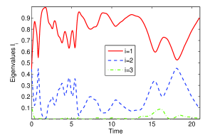
Figure 8: (Color online) Time evolution of the eigenvalues $I_{i}$ (see Eq. (25) for their definition) of one particular four-particle cluster.

The particle tracks ${\bm{x}}_{1}(t)$, ${\bm{x}}_{2}(t)$, ${\bm{x}}_{3}(t)$, and ${\bm{x}}_{4}(t)$ can be transformed into the center-of-mass coordinate

$${\bm{r}}(t)=\frac{1}{4}\sum_{i=1}^{4}{\bm{x}}_{i}(t)\,,$$ (22)

and the three relative coordinates (which are of interest here)

$${\bm{\rho}}_{1}(t) = \frac{1}{\sqrt{2}}[{\bm{x}}_{2}(t)-{\bm{x}}_{1}(t)]\,$$

$${\bm{\rho}}_{2}(t) = \frac{1}{\sqrt{6}}[2{\bm{x}}_{3}(t)-{\bm{x}}_{1}(t)-{\bm{x}}_{2}(t)]\,$$

$${\bm{\rho}}_{3}(t) = \frac{1}{\sqrt{12}}[3{\bm{x}}_{4}(t)-{\bm{x}}_{1}(t)-{\bm{x}}_{2}(t)-{\bm{x}}_{3}(t)]\,.$$ (23)

The radius of gyration follows in this frame to $R_{g}=\sqrt{\rho_{1}^{2}+\rho_{2}^{2}+\rho_{3}^{2}}$. The shape evolution of the particle cluster is monitored by the following moment-of-inertia tensor

$$g^{ab}=\sum_{i=1}^{3}\rho_{i}^{a}\rho_{i}^{b}\,,$$ (24)

where $a,b=x,y,z$ is the component index of the vector ${\bm{\rho}}_{i}$ and $i=1,2,3$. The real eigenvalues $g_{1}\geq g_{2}\geq g_{3}\geq 0$ quantify the shape of the particle cluster. Isotropic objects correspond with $g_{1}=g_{2}=g_{3}$, cigar-shaped clusters with $g_{1}\gg g_{2}\approx g_{3}$ and pancake-shaped clusters with $g_{1}\approx g_{2}\gg g_{3}$. Figure 8 shows the time evolution of the three eigenvalues for one specific 4-particle cloud. The eigenvalues are normalized and given by

$$I_{k}=\frac{g_{k}}{\sum_{m=1}^{3}g_{m}}\;\;\;\mbox{for}\;\;\;k=1,2,3\,.$$ (25)

Thus $0\leq I_{k}\leq 1$. One can observe, that the eigenvalue variations become smoother with increasing time. A convergence of the cluster to an almost coplanar object is observable for larger times, as quantified by the small value of $I_{3}$ . It will turn out now that this example displays a typical long-time behavior.

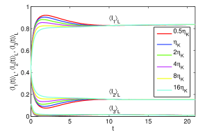
Figure 9: (Color online) Time evolution of the normalized eigenvalues of the moment-of-inertia tensor. The average is taken over the whole ensemble of tetrahedra. For times $t>10(=87\tau_{\eta})$ the data converge to values $\langle I_{3}\rangle_{L}\to 0.84$, $\langle I_{2}\rangle_{L}\to 0.15$, and $\langle I_{1}\rangle_{L}\to 0.01$. The tetrahedra are seeded in the whole volume initially.

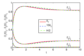
Figure 10: (Color online) Time evolution of the normalized eigenvalues of the moment-of-inertia tensor. The average is taken again over the whole ensemble of $5\times 10^{4}$ tetrahedra for each case. Four tracer particles form initially a tetrahedron with a sidelength of $\eta_{K}/2$. Three ensembles started in planes with $\delta$, 10$\delta_{T}$ and $H/2$ as given in the legend.

In Fig. 9, we show the time evolution of the Lagrangian ensemble average of the normalized eigenvalues. Data for different initial sidelengths of the tetrahedra are compared. The tetrahedra are seeded across the whole volume. Similar to the two-point measure, the initial deformation of the clusters depends sensitively on the sidelength of the tetrahedron. The smaller the initial sidelength the stronger the initial stretching of the cluster to a cigar-shaped object (for $t\lesssim 15\tau_{\eta}$). After about $87\tau_{\eta}$ all curves collapse and the mean values remain almost unchanged. Our data yield $\langle I_{1}\rangle_{L}=0.84$, $\langle I_{2}\rangle_{L}=0.15$, $\langle I_{3}\rangle_{L}=0.01$. Suprisingly, the obtained mean values are very close to the findings of Biferale et al. Biferale2005 and Hackl et al. Hackl2008 for homogeneous isotropic turbulence. In Ref. Biferale2005 , tetrahedra were excluded that had two points too close or too far of each other such that their values are not directly comparable with the present ones. Recent three-dimensional particle tracking experiments by Lüthi et al. Luethi2007 report an $\langle I_{2}\rangle_{L}$ which is also close to 0.16.

Since the large scales are probed in the long-term limit by the particle clusters, this agreement suggests that convective and isotropic turbulence on this scale do not differ significantly. The relative motion within a cluster is insensitive to whether the tracer particles are swept by large vortex structures or by large-scale circulation. Consequently, our findings suggest that the constrained vertical motion (and thus the inhomogeneity) is not important in the diffusive long-time limit of the cluster dynamics.

One can expect that for times $t>10^{2}\tau_{\eta}$, the tracers advance independently of each other. The present long-time means are compared with the result of a joint Gaussian distribution of the relative coordinates, $p({\bm{\rho}_{1}},{\bm{\rho}_{2}},{\bm{\rho}_{3}})\sim\exp[-(\rho_{1}^{2}+\rho_{2}^{2}+\rho_{3}^{2})]$. This ansatz results to $\langle I_{1}\rangle_{G}=0.75$, $\langle I_{2}\rangle_{G}=0.22$, and $\langle I_{3}\rangle_{G}=0.03$ for the three-dimensional case which is obtained by Monte-Carlo simulations Pumir2000 . The reported mean of $\langle I_{2}\rangle_{L}=0.15$ is smaller than the Gaussian value.

Figure 10 reports the dependence of the shape evolution from the initial position $z_{0}$. The effects remain small, but systematic. The closer the starting position of the tetrahedron to the boundary plane, the faster it converges into the final quasistatic state. Again the stretching and deformation is most efficient when the particle cluster passes through the mixing zone right above the tnermal boundary layer.

Figure 11 displays the PDFs of $I_{k}$ for five instants $t>87\tau_{\eta}$. The plots highlight two aspects. First, there is still a big variety in the amplitudes of individual $I_{k}$ although their means remain almost unchanged. Second, a very slow drift in the tails is present which is indicated by the arrows in Fig. 8(a) and (c).

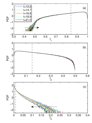
Figure 11: (Color online) Probability density functions of the normalized eigenvalues $I_{k}$ of the moment-of-inertia tensor (a) $I_{1}$, (b) $I_{2}$, and (c) $I_{3}$. The time instants at which the data have been analysed are for $t>87\tau_{\eta}$ as given in the legend in (a). The vertical dashed lines mark the long-time averages $\langle I_{k}\rangle_{L}$. The arrows in the upper and lower panel indicate that there is still a slight drift in the tails although the means in Fig. 9 remain nearly unchanged. The tetrahedra are seeded again in the whole volume initially.

V Acceleration statistics

The top panel of Fig. 12 shows the PDFs of the three acceleration components. Each component is given in units of the corresponding root-mean-square value. As expected, the distributions of the two lateral components coincide. Table 1 provides the quantitative details of the acceleration statistics and lists for example the skewness $S(a_{k})=\langle a_{k}^{3}\rangle/\langle a_{k}^{2}\rangle^{3/2}$ and the flatness $F(a_{k})=\langle a_{k}^{4}\rangle/\langle a_{k}^{2}\rangle^{2}$ with $k=x,y$ or $z$. The numbers for the lateral components are almost identical. The vertical acceleration component has a smaller flatness which is in line with a sparser tail of the corresponding PDF. The bottom panel of the same figure provides the statistical convergence test of the fourth-order moments where the product $w^{4}p(w)$ is plotted vs. $w$ with $w=a_{k}/a_{k,rms}$. It reflects the fundamental difficulty to gather reliable statistics for higher-order moments in Lagrangian turbulence. Recall that this analysis is conducted over a set of $4.4\times 10^{8}$ events. The area which is occupied by the scatter of the graphs in the tails of the PDFs determines the error bar of the fourth-order moment (and consequently of the flatness). We checked that the second and third-order moments display almost no scatter (not shown). The issue of statistical convergence has been discussed for turbulence measurements in a swirling flow Voth2002 ; Mordant2004 and in numerical simulations of homogeneous isotropic turbulence Toschi2005 . Our values for the flatness $F(a_{k})$ of the lateral flatness are of the same magnitude as those reported in Voth2002 .

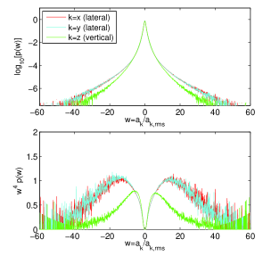
Figure 12: (Color online) Probability density function (PDF) of acceleration components $a_{k}$ with $k=x,y$ and $z$. Upper panel: PDF plots. Each component is normalized by its corresponding root-mean-square value. Lower panel: Statistical convergence test for the 4th moment of the acceleration. The total number of events which as been included for the analysis are $4.4\times 10^{8}$.

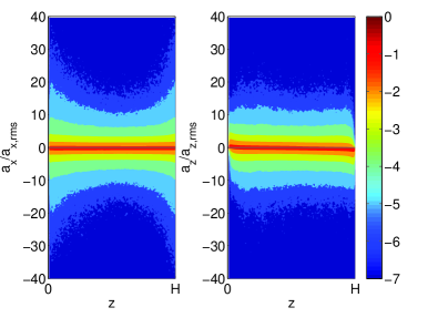
Figure 13: (Color online) Joint probability density function of acceleration components $a_{i}$ and the height $z$. Left: component $a_{x}$. Right: component $a_{z}$. The contours are displayed units of the decadic logarithm. The normalization of the acceleration component in both panels is as in Fig. 12.

	$\sqrt{\langle a_{k}^{2}\rangle}$	$\frac{\max(a_{k})}{g}$	$\frac{\min(a_{k})}{g}$	$S(a_{k})$	$F(a_{k})$
$a_{x}$	1.17	1001	-574	-0.093	63.4 ($\pm$ 16)
$a_{y}$	1.16	559	-540	-0.156	64.4 ($\pm$ 16)
$a_{z}$	1.10	518	-680	-0.119	30.3 ($\pm$ 11)

Table 1: Root-mean-square values, total maximum/minimum amplitudes, skewness $S(a_{k})=\langle a_{k}^{3}\rangle/\langle a_{k}^{2}\rangle^{3/2}$ and flatness $F(a_{k})=\langle a_{k}^{4}\rangle/\langle a_{k}^{2}\rangle^{2}$ of the acceleration components. The error bars of $F(a_{k})$ have been obtained by measuring the area of the scatter in the lower panel of Fig. 12. Maxima and mininma are given in units of the gravity acceleration $g$.

Figure 13 refines the statistical analysis of the acceleration components. Due to the vertical inhomogeneity, we report the height dependence of the acceleration statistics for one lateral and the vertical component, respectively, and plot contours of the joint PDF $p(a_{i},z)$. The largest lateral accelerations and the fattest tails are found close to the top and bottom planes. It will turn out in the next section that the vorticity is concentrated in cyclones and anti-cyclones close to the thermal boundary layer which can rationalize the large lateral accelerations. The support of the PDF decreases monotonically to the center plane. We will get back to this point later in the text when discussing the role of the vertical vorticity component in connection with plume detachments. In contrast to the result for the lateral accelerations, the support of the joint PDF $p(a_{z},z)$ shows no significant variation with height. It shrinks to zero in the boundary planes (since is $u_{z}\equiv 0$) and grows rapidly up to about the thermal boundary layer thickness. The slight asymmetry of the inner contour lines (for the largest probability density levels) corresponds with the rising plumes which detach from the bottom plane at $z=0$ and have $a_{z}>0$ and with falling plumes at $z=H$ for which $a_{z}<0$. Note also that the support of all pdfs is the same in the center of the cell. This is consistent with the idea that the turbulence is close to isotropic far away from the isothermal walls.

The important result of this section is that there is differently strong intermittency for the vertical and lateral accelerations in thermal convection. It is caused by the higher level of intermittency in and close to the thermal boundary layer. As a consequence, we will have to take a closer look at the mechanisms of local heat transfer in the vicinity of the top and bottom planes. This is done in the next section.

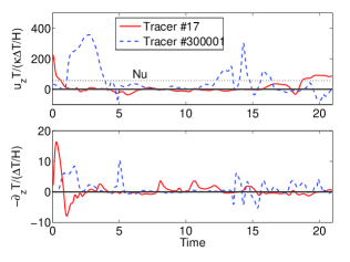
Figure 14: (Color online) Time traces of the convective (top) and conductive (bottom) heat transfer along two of the $1.2\times 10^{6}$ tracers. The Eulerian value of $Nu$ is indicated as a dotted line in the top panel.

VI Lagrangian convective and conductive heat flux

VI.1 Lagrangian heat flux

The local heat flux contributions can be probed in the Lagrangian frame of reference. We adopt therefore definition (10) and calculate the local Lagrangian conductive and convective flux contributions. They are given by

$$Nu({\bm{x}}) = Nu_{conv}({\bm{x}})+Nu_{cond}({\bm{x}})$$ (26)

$$= \frac{H}{\kappa\Delta T}(u_{z}({\bm{x}})T({\bm{x}})-\kappa\partial_{z}T({\bm{x}}))\,,$$

along the Lagrangian tracks ${\bm{x}}(t)$. Figure 14 shows typical time traces of $Nu_{conv}$ and $Nu_{cond}$ along two tracers. They display a big variability with respect to time. Even negative values are possible for both contributions. As expected, the convective term has a significantly larger magnitude than the conductive one. The latter is dominant in the thermal boundary layers where the thermal dissipation rate $\chi$ has the largest magnitude. Figure 15 displays the PDFs of the convective and conductive contributions gathered along the tracks of the whole tracer ensemble. In addition, we display the results for the products $u_{x}T$ and $u_{y}T$. All quantities are shown in units of their root-mean-square values. While the PDFs for $u_{x}T$ and $u_{y}T$ are symmetric, those of $u_{z}T$ and $\kappa\partial_{z}T$ are strongly skewed. This reflects the vertical net transfer of heat through the volume. The Lagrangian average $Nu_{L}=\langle Nu({\bm{x}})\rangle_{L,t}$ results to

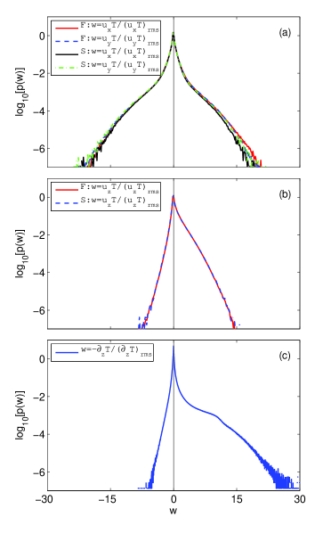
Figure 15: (Color online) Probability density functions (PDF) of the conductive and conductive heat flux contributions along the Lagrangian tracer tracks. (a) Lateral convective contributions $u_{x}T$ and $u_{y}T$. (b) Vertical convective contribution $u_{z}T$. (c) Conductive contribution $-\partial T/\partial z$. All quantities are normalized by their root-mean-square values. The analysis is conducted over two different data sets: the full record (F) and a third of it (S).

$$Nu_{L}=1+\frac{H}{\kappa\Delta T}\langle u_{z}T\rangle_{L,t}\,.$$ (27)

We have directly verified from the corresponding PDF in Fig. 15(c) that the mean of the Lagrangian conductive heat transfer is with 1.04 very close to one. Furthermore, it is found that $Nu_{L}<Nu$. This is in contrast to the experimental findings for the smart particle probe of Gasteuil et al. Gasteuil2007 where $Nu<Nu_{L}$. The reason for this difference might be due to the finite extension of the smart particle that exceeded the thickness of the thermal boundary layer. We have compared the result for the full record (F) with that of a smaller subset (S) which is one third of set (F) and the results differed by 6.5 % only (see also Fig. 15). A time-resolved analysis shows that $Nu_{L}(t)=\langle Nu({\bm{x}},t)\rangle_{L}$ relaxes slowly to the Eulerian value of $Nu$. The tracers which have been seeded randomly or at particular heights at the beginning have to pass a kind of “thermalization” process.

Our result sheds interesting light on the joint velocity-temperature sampling properties of the Lagrangian tracers. First, it is known that for the present geometry a large-scale circulations are present Hartlep2005 ; Reeuwijk2008 . Tracers will preferentially follow the circulation motion in the convection layer. The large-scale circulation can carry a fraction of the total heat transport only, as has been analyzed recently with a Proper Orthogonal Decomposition Bailon2009 . Second, we observe high-amplitude events of the vertical vorticity $\omega_{z}=\partial_{x}u_{y}-\partial_{y}u_{x}$ close to the maxima of the thermal dissipation rate $\chi$. This is shown in Figs. 16 and 17 where contour plots of slice snapshots of $\chi$ and $\omega_{z}$ at a height $z=\delta_{T}$ are compared. The local maxima in the dissipation rate plot (16) reproduce the skeleton of plume sheets. In their vicinity, we observe cyclones and anti-cyclones that are generated in connection with the detachment of plume fragments. This observation is in line with results in Shishkina2008 for the non-rotating and with Julien1996 for the rotating case. Exactly these cyclones and anti-cyclones cause the large lateral positive and negative accelerations as seen in the PDFs in Fig. 12. Fig. 18 plots vertical profiles of means of both quantities. While the root-mean-square of the vertical vorticity component varies weakly, the thermal dissipation rate is strongly peaked in and close to the boundary layer. It is also known from studies in homogeneous isotropic turbulence Toschi2009 that the Lagrangian tracers are not very frequently trapped in the core of such vortex structures.

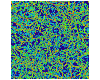
Figure 16: (Color online) Contour plot of the decadic logarithm of the thermal dissipation rate $\log_{10}[\chi(x,y,z=\delta_{T},t_{0})]$. The logarithmic contour spacing is chosen in order to highlight the small amplitude events.

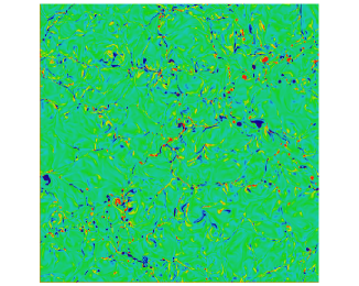
Figure 17: (Color online) Contour plot of the vertical vorticity component $\omega_{z}(x,y,z=\delta_{T},t_{0})$. Data correspond to those in Fig. 13.

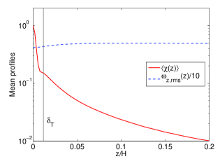
Figure 18: (Color online) Vertical profiles of the averaged thermal dissipation rate $\langle\chi(z)\rangle_{A,t}$ (solid line) and the root-mean-square of vertical vorticity component $\sqrt{\langle\omega^{2}(z)\rangle_{A,t}}$ (dashed line). The latter is divided by a factor of 10.

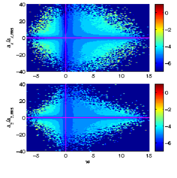
Figure 19: (Color online) Joint probability density function of the lateral acceleration (upper panel) and vertical (lower panel) acceleration and heat flux contributions. Upper panel: $w=u_{z}T/(u_{z}T)_{rms}$. Lower panel: $w=u_{z}T/(u_{z}T)_{rms}$. The contour spacing is in decadic logarithm.

VI.2 Joint statistics of Lagrangian heat flux and acceleration

The thermal plumes detach permantly from the thermal boundary layer and can be identified as regions in which the product $u_{z}T^{\prime}>0$ Gasteuil2007 ; Schumacher2008 . Here we extend this analysis and study the correlations between the vertical velocity component and the (total) temperature in relation to the acceleration. Figure 19 displays the joint statistics of the vertical and lateral accelerations and the products of velocity and temperature fluctuations, $u_{z}T$. In order to highlight the statistical correlation between the two variables of the joint PDF we divide the joint PDF by the two single quantity PDFs,

$$\Pi(a_{i},u_{z}T)=\frac{p(a_{i},u_{z}T)}{p(a_{i})p(u_{z}T)}\,.$$ (28)

The top panel of Fig. 19 shows the joint statistics for $a_{x}$ and $u_{z}T$. A pronunced maximum at larger accelerations and values of $u_{z}T$ is found. They can be related to coherent structures, such as vorticity tubes in the bulk of the slab or the cyclones/anti-cyclones in the boundary layer. The correlation between vertical acceleration and the product $u_{z}T$ is weaker. The local amplitudes of the joint PDF found at the outer boundaries of the support, at moderate acceleration amplitudes and larger values of $u_{z}T$. In Ref. Schumacher2008 , we reported the same behavior for $p(a_{z},u_{z}T^{\prime})$ and identified rising plumes $(a_{z}>0,u_{z}T^{\prime}>0)$ and falling plumes $(a_{z}<0,u_{z}T^{\prime}>0)$. Recirculations around rising and falling plumes have to form due to the incompressibility of the fluid. They were related to maxima in the halfplane $u_{z}T^{\prime}<0$. These are only some of the possible scenarios which can be assigned to strong correlations in the joint statistics. The firm conclusion which we can draw from the present analysis and the one in Schumacher2008 is that plumes (and therefore the vertical convective flux events) are not connected with the largest vertical accelerations. The detachment of plumes is a more gradual process.

We repeated the joint statistical analysis for the conductive part, $-\kappa\partial_{z}T({\bm{x}})$. Results are summarized in Fig. 20. The contour plots display now

$$\Pi(a_{z},-\partial_{z}T)=\frac{p(a_{z},-\partial_{z}T)}{p(a_{z})p(-\partial_{z}T)}\,.$$ (29)

We keep in mind from (10) and (26) that upward conductive heat transport events have a negative sign, i.e. $-|\partial_{z}T|$. While the lower panel of Fig. 20 includes the Lagrangian data of the whole volume, the upper panel of the same figure excludes events in the thermal boundary layer up to the beginning of the plume mixing zones. This zone was identified and studied in Schumacher2008 and starts for the present parameter setting at a height H/16. The extended tail in the lower panel can thus be related to largest gradients (and thus largest thermal dissipation rate amplitudes) in and above the thermal boundary layer. The asymmetry to negative $a_{z}$ for the largest gradients can be interpreted as tracer decelerations which are present when temperature gradients are formed. Negative accelerations (or decelerations) seem to be frequently related to stagnation-point flow topologies, those flows which can steepen the temperature field to large gradients.

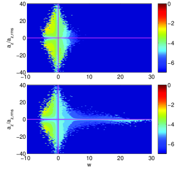
Figure 20: (Color online) Joint probability density function of the vertical acceleration component $a_{z}/a_{z,rms}$ and $w=-\partial_{z}T/(\partial_{z}T)_{rms}$. Top panel: Tracer positions in the bulk have been considered only. Bottom panel: Tracer positions in the whole volume are included. The contour spacing is in decadic logarithm.

VII Summary and discussion

The focus of the present work was on Lagrangian aspects of turbulent convection. The results can be summarized as follows. The study of pair and multiparticle dispersion yields qualitatively similar results compared to the homogeneous isotropic case. Although the scaling behavior of second order moments is sensitive to initial separations and seeding heights, initial separations close to the Kolmogorov length result in a short Richardson-like scaling range. Interestingly, we reproduce the same long-time limits for the particle cluster shapes as in isotropic turbulence despite turbulent convection is inhomogeneous. This limit deviates from the Gaussian value. Our results suggest that the dispersion laws can be obtained for more complex flows than isotropic homogeneous turbulence. The proportionality constants are however different which can be attributed to qualitaively different turbulence structures such as thermal plumes in convection. They affect the vertical dispersion more significantly than the lateral dispersion.

The inhomogeneity of the convective turbulence manifests in less intermittent statistics of the vertical acceleration component compared to the lateral ones. Thermal plumes are not coupled with the strongest accelerations.

We find that the Lagrangian Nusselt number converges slowly to the Eulerian value. A closer inspection of this point could be done in several steps: first, to disentangle the large-scale circulation from the turbulent background, as done in Bailon2009 , and to combine such a study with a Lagrangian analysis. Second, the present study indicates also that the Nusselt number relaxes faster with a growing number of tracers, in other words the sampling of joint velocity-temperature statistics improves. Our observation is also related to recent experimental and numerical studies at very large Rayleigh numbers Amati2005 ; Niemela2008 in which the existence and growth of a so-called superconducting core is discussed, which is in line with a decreasing importance of the large flow circulation for growing Rayleigh numbers. A decreasing importance of a coherent large-scale circulation might lead again to a faster convergence $Nu_{L}\rightarrow Nu$. More studies of the Lagrangian frame of high-Rayleigh number turbulence are thus necessary.

- (1) L. P. Kadanoff, Phys. Today 54, 34 (2001).
- (2) G. Ahlers, S. Grossmann, and D. Lohse, Rev. Mod. Phys., to be published.
- (3) O. Shishkina and C. Wagner, Phys. Fluids 19, 085107 (2007).
- (4) S.-Q. Zhou, C. Sun, and K.-Q. Xia, Phys. Rev. Lett. 98, 074501 (2007).
- (5) O. Shishkina and C. Wagner, J. Fluid Mech. 599, 383 (2008).
- (6) M. S. Emran and J. Schumacher, J. Fluid Mech. 611, 13 (2008).
- (7) R. M. Kerr, J. Fluid Mech. 310, 139 (1996).
- (8) J. J. Niemela, L. Skrbek, K. R. Sreenivasan, and R. J. Donelly, Nature 404, 837 (2000).
- (9) G. Amati, K. Koal, F. Massaioli, K. R. Sreenivasan, and R. Verzicco, Phys. Fluids 17, 121701 (2005).
- (10) D. Funfschilling, E. Brown, A. Nikolaenko, and G. Ahlers, J. Fluid Mech. 536, 145 (2005).
- (11) F. Toschi and E. Bodenschatz, Annu. Rev. Fluid Mech. 41, 375 (2009).
- (12) K. R. Sreenivasan and J. Schumacher, Phil. Trans. Roy. Soc., to be published.
- (13) S. Ott and J. Mann, J. Fluid Mech. 422, 207 (2000).
- (14) A. La Porta, G. A. Voth, A. M. Crawford, J. Alexander, and E. Bodenschatz, Nature 409, 1017 (2001).
- (15) M. Guala, B. Lüthi, A. Liberzon, A. Tsinober, and W. Kinzelbach, J. Fluid Mech. 533, 339 (2005).
- (16) N. Mordant, P. Metz, O. Michel und J.-F. Pinton, Phys. Rev. Lett. 87, 214501 (2001).
- (17) P. K. Yeung, Annu. Rev. Fluid Mech. 34, 115 (2002).
- (18) G. Boffetta and I. M. Sokolov, Phys. Rev. Lett. 88, 094501 (2002).
- (19) L. Biferale, G. Boffetta, A. Celani, B. J. Devinish, A. Lanotte, and F. Toschi, Phys. Fluids 17, 115101 (2005).
- (20) B. L. Sawford, P. K. Yeung, and J. F. Hackl, Phys. Fluids 20, 065111 (2008).
- (21) Y. Gasteuil, W. L. Shew, M. Gibert, F. Chillá, B. Castaing, and J.-F. Pinton, Phys. Rev. Lett. 93, 234302 (2007).
- (22) E. Calzavarini, D. Lohse, F. Toschi, and R. Tripiccione, Phys. Fluids 17, 055107 (2005).
- (23) E. Calzavarini, C. R. Doering, J. D. Gibbon, D. Lohse, A. Tanabe, and F. Toschi, Phys. Rev. E 73, 035301 (2006).
- (24) J. Schumacher, Phys. Rev. Lett. 100, 134502 (2008).
- (25) B. Castaing, G. Gunarante, F. Heslot, L. P. Kadanoff, A. Libchaber, S. Thomae, X.-Z. Wu, S. Zaleski, and G. Zanetti, J. Fluid Mech. 204, 1 (1989).
- (26) S.-Q. Zhou and K.-Q. Xia, Phys. Rev. Lett. 89, 184502 (2002).
- (27) M. Chertkov, A. Pumir, and B. I. Shraiman, Phys. Fluids 11, 2394 (1999).
- (28) A. Pumir, B. I. Shraiman, and M. Chertkov, Phys. Rev. Lett. 85, 5324 (2000).
- (29) J. Schumacher and M. Pütz, Turbulence in laterally extended systems, in Proceedings of the International Conference ParCo 2007, Eds. C. Bischof, M. Bücker, P. Gibbon, G. Joubert, T. Lippert, B. Mohr, F. Peters, IOS Press, Amsterdam, 585 (2007).
- (30) http://www.sdsc.edu/us/resources/p3dfft/index.php
- (31) K. Julien, S. Legg, J. Mc Williams, and J. Werne, J. Fluid Mech. 322, 243 (1996).
- (32) M. Bourgoin, N. T. Ouelette, H. Xu, J. Berg, and E. Bodenschatz, Science 311, 835 (2006).
- (33) L. F. Richardson, Proc. Roy. Soc. London Ser. A 110, 709 (1926).
- (34) G. K. Batchelor, Q. J. R. Meteorol. Soc. 76, 133 (1950).
- (35) J. R. Cressman, W. I. Goldburg, and J. Schumacher, Europhys. Lett. 66, 219 (2004).
- (36) J. F. Hackl, P. K. Yeung, B. L. Sawford, and M. S. Borgas, Bull. Am. Phys. Soc. 53 (15), 298 (2008).
- (37) B. Lüthi, S. Ott, J. Berg, and J. Mann, J. Turb. 8, 45 (2007).
- (38) G. A. Voth, A. La Porta, A. M. Crawford, J. Alexander, and E. Bodenschatz, J. Fluid Mech. 469, 121 (2002).
- (39) N. Mordant, A. M. Crawford, and E. Bodenschatz, Physica D 193, 245 (2004).
- (40) T. Hartlep, A. Tilgner, and F. H. Busse, J. Fluid Mech. 544, 309 (2005).
- (41) M. van Reeuwijk, H. J. J. Jonker, and K. Hanjalić, Phys. Rev. E 77, 036311 (2008).
- (42) J. Bailon-Cuba, M. S. Emran, and J. Schumacher, J. Fluid Mech., submitted (2009).
- (43) F. Toschi, L. Biferale, G. Boffetta, A. Celani, B. J. Devenish, and A. Lanotte, J. Turb. 6, 40 (2005).
- (44) J. J. Niemela and K. R. Sreenivasan, Phys. Rev. Lett. 100, 184502 (2008).