Curvature-enhanced spin-orbit coupling in a carbon nanotube

Abstract

Structure of the spin-orbit coupling varies from material to material and thus finding the correct spin-orbit coupling structure is an important step towards advanced spintronic applications. We show theoretically that the curvature in a carbon nanotube generates two types of the spin-orbit coupling, one of which was not recognized before. In addition to the topological phase-related contribution of the spin-orbit coupling, which appears in the off-diagonal part of the effective Dirac Hamiltonian of carbon nanotubes, there is another contribution that appears in the diagonal part. The existence of the diagonal term can modify spin-orbit coupling effects qualitatively, an example of which is the electron-hole asymmetric spin splitting observed recently, and generate four qualitatively different behavior of energy level dependence on parallel magnetic field. It is demonstrated that the diagonal term applies to a curved graphene as well. This result should be valuable for spintronic applications of graphitic materials.

I introduction

Graphitic materials such as carbon nanotubes (CNTs) and graphenes are promising materials for spintronic applications. Various types of spintronic devices are reported such as CNT-based three terminal magnetic tunnel junctions Sahoo05NaturePhysics , spin diodes Merchant08PRL , and graphene-based spin valves Tombros07Nature . Graphitic materials are believed to be excellent spin conductors Tsukagoshi99Nature . The hyperfine interaction of electron spins with nuclear spins is strongly suppressed since ¹²C atoms do not carry nuclear spins. It is estimated that the spin relaxation time in a CNT Bulaev08PRB and a graphene Hernando08Condmat is limited by the spin-orbit coupling (SOC).

Carbon atoms are subject to the atomic SOC Hamiltonian $H_{\rm so}$. In an ideal flat graphene, the energy shift caused by $H_{\rm so}$ is predicted to be $\sim 10^{-3}$ meV Min06PRB ; Hernando06PRB . Recently it is predicted Hernando06PRB ; Ando00JPSJ that the geometric curvature can enhance the effective strength of the SOC by orders of magnitude. This mechanism applies to a CNT and also to a graphene which, in many experimental situations, exhibits nanometer-scale corrugations Meyer07Nature . There is also a suggestion Pereira08arXiv that artificial curved structures of a graphene may facilitate device applications.

A recent experiment Kuemmeth08Nature on ultra-clean CNTs measured directly the energy shifts caused by the SOC, which provides an ideal opportunity to test theories of the curvature-enhanced SOC in graphitic materials. The measured shifts are in order-of-magnitude agreement with the theoretical predictions Ando00JPSJ ; Hernando06PRB , confirming that the curvature indeed enhances the effective SOC strength. The experiment revealed discrepancies as well; While existing theories predict the same strength of the SOC for electrons and holes, which is natural considering that both the conduction and valence bands originate from the same $\pi$ orbital, the experiment found considerable asymmetry in the SOC strength between electrons and holes. This electron-hole asymmetry implies that existing theories of the SOC in graphitic materials are incomplete.

In this paper, we show theoretically that in addition to effective SOC in the off-diagonal part of the effective Dirac Hamiltonian, which was reported in the existing theories Ando00JPSJ ; Hernando06PRB , there exists an additional type of the SOC that appears in the diagonal part both in CNTs and curved graphenes. It is demonstrated that the combined action of the two types of the SOC produces the electron-hole asymmetry observed in the CNT experiment Kuemmeth08Nature and gives rise to four qualitatively different behavior of energy level dependence on magnetic field parallel to the CNT axis.

This paper is organized as follows. In Sec. II, we show analytical expressions of two types of the effective SOC in a CNT and then explain how the electron-hole asymmetric spin splitting can be generated in semiconducting CNTs generically. Section III describes the second-order perturbation theory that is used to calculate the effective SOC, and tight-binding models of the atomic SOC and geometric curvature. Section IV reports four distinct energy level dependence on magnetic field parallel to the CNT axis. We conclude in Sec. V with implications of our theory on curved graphenes and a brief summary.

II Effective spin-orbit coupling in a CNT

We begin our discussion by presenting the first main result for a CNT with the radius $R$ and the chiral angle $\theta$ ($0\!\leq\!\theta\!\leq\!\pi/6$, $0\,(\pi/6)$ for zigzag (armchair) CNTs). We find that when the two sublattices $A$ and $B$ of the CNT are used as bases, the curvature-enhanced effective SOC Hamiltonian ${\cal H}_{\rm soc}$ near the K point with Bloch momentum ${\bf K}$ becomes

$${\cal H}_{\rm soc}^{\rm K}=\left(\begin{array}[]{cc}(\delta^{\prime}_{\rm K}/R)\sigma_{y}&(\delta_{\rm K}/R)\sigma_{y}\\ (\delta^{*}_{\rm K}/R)\sigma_{y}&(\delta^{\prime}_{\rm K}/R)\sigma_{y}\end{array}\right),$$ (1)

where $\sigma_{y}$ represents the real spin Pauli matrix along the CNT axis. The pseudospin is defined to be up (down) when an electron is in the sublattice $A\,(B)$. Here the off-diagonal term that can be described by a spin-dependent topological phase are reported in Refs. Hernando06PRB ; Ando00JPSJ but the diagonal term was not recognized before. Expressions for the parameters $\delta_{\rm K}$ and $\delta^{\prime}_{\rm K}$ are given by comment-delta

$${\delta_{\rm K}\over R}=\frac{\lambda_{\rm so}a(\varepsilon_{s}-\varepsilon_{p})(V_{pp}^{\pi}+V_{pp}^{\sigma})}{12\sqrt{3}{V_{sp}^{\sigma}}^{2}}\frac{e^{-i\theta}}{R}$$ (2)

and

$${\delta^{\prime}_{\rm K}\over R}=\frac{\lambda_{\rm so}aV_{pp}^{\pi}}{2\sqrt{3}(V_{pp}^{\sigma}-V_{pp}^{\pi})}\frac{\cos 3\theta}{R},$$ (3)

where $\lambda_{\rm so}\sim 12\,$meV Serrano00SSC is the atomic SOC constant, $a$ is the lattice constant $2.49{\AA}$, and $\varepsilon_{s(p)}$ is the atomic energy for the $s(p)$ orbital. Here, $V_{sp}^{\sigma}$ and $V_{pp}^{\pi(\sigma)}$ represent the coupling strengths in the absence of the curvature for the $\sigma$ coupling between nearest neighbor $s$ and $p$ orbitals and the $\pi$($\sigma$) coupling between nearest neighbor $p$ orbitals, respectively. Note that the $|\delta^{\prime}_{\rm K}|$ has the $\theta$-dependence, whose implication on the CNT energy spectrum is addressed in Sec. IV. For K^′ point with ${\bf K^{\prime}}\!=\!-{\bf K}$, ${\cal H}_{\rm soc}^{\rm K^{\prime}}$ is given by Eq. (1) with $\delta_{\rm K}$ and $\delta_{\rm K}^{\prime}$ replaced by $\delta_{\rm K^{\prime}}\!=\!-\delta^{*}_{\rm K}$ and $\delta^{\prime}_{\rm K^{\prime}}\!=\!-\delta^{\prime}_{\rm K}$, respectively.

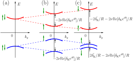
Figure 1: (Color online) Schematic diagram of the lowest conduction (red, $E>0$) and highest valence (blue, $E<0$) band positions of a semiconducting CNT predicted by ${\cal H}_{\rm Dirac}^{\rm K}+{\cal H}_{\rm soc}^{\rm K}$ for (a) $\delta_{\rm K}\!=\!\delta^{\prime}_{\rm K}\!=\!0$, (b) $\delta_{\rm K}\!\neq\!0$, $\delta^{\prime}_{\rm K}\!=\!0$, and (c) $\delta_{\rm K}\!\neq\!0$, $\delta^{\prime}_{\rm K}\!\neq\!0$. In (c), the conduction or valence band has larger spin splitting depending on the sign of $\nu$. Arrows (green) show the spin direction along the CNT. The expressions for the energy level spacing are also provided. When they are negative, the positions of the two spin-split bands should be swapped.

Implications of the diagonal term of the SOC become evident when Eq. (1) is combined with the two-dimensional Dirac Hamiltonian ${\cal H}_{\rm Dirac}$ of the CNT. For a state near the K point with the Bloch momentum $\mathbf{K}+\mathbf{k}$ [$\mathbf{k}=(k_{x},k_{y})$, $|\mathbf{k}|\ll|\mathbf{K}|$], ${\cal H}_{\rm Dirac}$ becomes Ajiki93JPSJ

$${\cal H}_{\rm Dirac}^{\rm K}=\hbar v_{\rm F}\left(\begin{array}[]{cc}0&e^{-i\theta}(k_{x}-ik_{y})\\ e^{+i\theta}(k_{x}+ik_{y})&0\end{array}\right),$$ (4)

where $v_{F}$ is the Fermi velocity and the momentum component $k_{x}$ along the circumference direction satisfies the quantization condition $k_{x}={(1/3R})\nu$ for a $(n,m)$ CNT with $n-m=3q+\nu$ ($q\in\mathbb{Z}$ and $\nu=\pm 1,0$) and $\theta=\tan^{-1}[{\sqrt{3}m/(2n+m)}]$. For a semiconducting $(\nu\!=\!\pm 1)$ CNT, the diagonalization of ${\cal H}_{\rm Dirac}^{\rm K}\!+\!{\cal H}_{\rm soc}^{\rm K}$ results in different spin splittings [Fig. 1(c)] of $-2\delta^{\prime}_{\rm K}/R-2\nu{\rm Re}[\delta_{\rm K}e^{i\theta}]/R$ and $2\delta^{\prime}_{\rm K}/R-2\nu{\rm Re}[\delta_{\rm K}e^{i\theta}]/R$ for the conduction and valence bands, respectively. This explains the electron-hole asymmetry observed in the recent experiment Kuemmeth08Nature . Here we remark that neither the off-diagonal ($\delta_{\rm K}$) nor the diagonal ($\delta^{\prime}_{\rm K}$) term of the SOC alone can generate the electron-hole asymmetry since the two spin splittings can differ by sign at best, which actually implies the same magnitude of the spin splitting (see Fig. 1 for the sign convention). Thus the interplay of the two types is crucial for the asymmetry.

III Theory and Model

We calculate the $\delta_{\rm K}$ and $\delta^{\prime}_{\rm K}$ analytically using degenerate second-order perturbation theory and treating atomic SOC and geometric curvature as perturbation. For simplicity, we evaluate $\delta_{\rm K}$ and $\delta^{\prime}_{\rm K}$ in the limit ${\bf k}\!=\!0$. Although this limit is not strictly valid since ${\bf k}\!=\!0$ does not generally satisfy the quantization condition on $k_{x}$, one may still take this limit since the dependence of $\delta_{\rm K}$ and $\delta^{\prime}_{\rm K}$ on ${\bf k}$ is weak. An electron at the K point is described by the total Hamiltonian $H^{{\rm K},(0)}+H_{\rm so}+H_{\rm c}$, where $H_{\rm c}$ describes the curvature effects and $H^{{\rm K},(0)}$ describes the $\pi$ and $\sigma$ bands in the absence of both $H_{\rm so}$ and $H_{\rm c}$. The $\pi$ band eigenstates of $H^{{\rm K},(0)}$ are given by

$$|\Psi_{\uparrow(\downarrow)}^{{\rm K},(0)}\rangle=\frac{1}{\sqrt{2}}\left(\nu\,e^{-i\theta}\left|\psi_{A}^{\rm K}\right\rangle\pm\left|\psi_{B}^{\rm K}\right\rangle\right)\chi_{\uparrow(\downarrow)}$$ (5)

with the corresponding eigenvalues $E^{{\rm K},(0)}_{\uparrow(\downarrow)}\!\equiv\!E^{(0)}\!=\!0$. Here $|\Psi_{\uparrow(\downarrow)}^{{\rm K},(0)}\rangle$ with the upper (lower) sign amounts to the ${\bf k}=0$ limit of the eigenstate at the the conduction band bottom (valence band top). $\chi_{\uparrow(\downarrow)}$ denotes the eigenspinor of $\sigma_{y}$. $|\psi_{A(B)}^{{\rm K}}\rangle={1\over\sqrt{N}}\sum_{r={\bf r}_{A(B)}}e^{i{\bf K}\cdot r}\left|p_{z}^{r}\right\rangle$ is the orbital projection of $|\Psi_{\uparrow(\downarrow)}^{{\rm K},(0)}\rangle$ into the sublattice $A\,(B)$, $|p_{z}^{r}\rangle$ represents the $p_{z}$ orbital at the atomic position $r$, and the $z$ axis is perpendicular to the CNT surface.

When $H_{\rm so}$ and $H_{\rm c}$ are treated as weak perturbations, the first order contribution $H_{\rm so}$ to the effective SOC vanishes since it causes the inter-band transition (Fig. 3) to the $\sigma$ band Hernando06PRB . The next leading order contribution to the effective SOC comes from the following second order perturbation Hamiltonian $H^{\rm K,(2)}$ Schiff68Book ,

$$H^{{\rm K},(2)}=H_{\rm c}\frac{\mathcal{P}^{\rm K}}{E^{(0)}-H^{{\rm K},(0)}}H_{\rm so}+{\rm H.c.},$$ (6)

where the projection operator $\mathcal{P}^{\rm K}$ is defined by $\mathcal{P}^{\rm K}\!\equiv\!1\!-\!\sum_{\alpha=\uparrow,\downarrow}|\Psi^{{\rm K},(0)}_{\alpha}\rangle\langle\Psi^{{\rm K},(0)}_{\alpha}|$. Another spin-dependent second order term $H_{\rm so}[\mathcal{P}^{\rm K}/(E^{(0)}\!-\!H^{{\rm K},(0)})]H_{\rm so}$ Second order Hamiltonian is smaller than Eq. (6) (by two orders of magnitude for a CNT with $R\!\sim\!2.5\,$nm), and thus ignored. Then the second order energy shift $E^{{\rm K},(2)}_{\uparrow(\downarrow)}$ is given by second-order energy correction-K'

$$E^{{\rm K},(2)}_{\uparrow} = \left\langle\psi_{A}^{{\rm K}}\right|\!H^{{\rm K},(2)}\!\left|\psi_{A}^{{\rm K}}\right\rangle\!\pm\!\nu{\rm Re}\!\left[\langle\psi_{A}^{{\rm K}}|H^{{\rm K},(2)}|\psi_{B}^{{\rm K}}\rangle e^{i\theta}\right]$$

$$E^{{\rm K},(2)}_{\downarrow} = -E^{{\rm K},(2)}_{\uparrow},$$ (7)

where the upper (lower) sign applies to the energy shift of the conduction band bottom (valence band top) and $\langle\psi_{A}^{{\rm K}}|H^{{\rm K},(2)}|\psi_{A}^{{\rm K}}\rangle\!=\!\langle\psi_{B}^{{\rm K}}|H^{{\rm K},(2)}|\psi_{B}^{{\rm K}}\rangle$ is used. Then by comparing $E^{{\rm K},(2)}_{\uparrow(\downarrow)}$ with Fig. 1, one finds

$$\frac{\delta_{\rm K}}{R}=\left\langle\psi_{A}^{\rm K}\right|\!H^{\rm K,(2)}\!\left|\psi_{B}^{\rm K}\right\rangle,\,\,\,\frac{\delta^{\prime}_{\rm K}}{R}=\left\langle\psi_{A}^{\rm K}\right|\!H^{{\rm K},(2)}\!\left|\psi_{A}^{\rm K}\right\rangle.$$ (8)

Note that $\delta_{\rm K}$ and $\delta^{\prime}_{\rm K}$ are related to pseudospin-flipping and pseudospin-conserving processes, respectively.

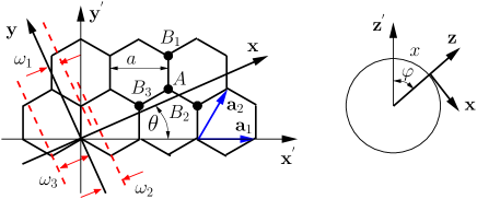
Figure 2: (Color online) Two-dimensional honeycomb lattice structure. ${\bf x}({\bf y})$ is the coordinate around (along) the CNT with chiral vector $n\,{\mathbf{a}_{1}}\!+\!m\,{\mathbf{a}_{2}}\!\equiv\!(n,m)$ and chiral angle $\theta$. $\omega_{j}\,(j\!=\!1,2,3)$, the length between $y$ axis passing $A$ atom and its parallel (red dashed) line is related with $\xi_{j}$ by $\xi_{j}\!\approx\!\omega_{j}/(2R)$ [Eq. (III)]. The coordinates for the CNT is illustrated on the right. Here, $x\!=\!\varphi R$.

To evaluate Eq. (8), one needs explicit expressions for $H_{\rm so}$, $H_{\rm c}$, and $H^{\rm K,(0)}$. $H_{\rm so}$ is given by $\lambda_{\rm so}\!\sum_{r}\mathbf{L}_{r}\!\cdot\!\mathbf{S}_{r}$ Min06PRB , where $\mathbf{L}_{r}$ and $\mathbf{S}_{r}$ are respectively the atomic orbital and spin angular momentum of an electron at a carbon atom $r$. The tight-binding Hamiltonian of the $H_{\rm so}$ can be written Hernando06PRB as $H_{\rm so}={(\lambda_{\rm so}/2)}\sum_{r={\bf r}_{A/B}}(c_{r-}^{z\dagger}c_{r+}^{x}-c_{r+}^{z\dagger}c_{r-}^{x}+ic_{r+}^{z\dagger}c_{r-}^{y}+ic_{r-}^{z\dagger}c_{r+}^{y}+ic_{r+}^{y\dagger}c_{r+}^{x}-ic_{r-}^{y\dagger}c_{r-}^{x})+{\rm H.c.}$, where $c_{r+(\!-\!)}^{x}$, $c_{r+(\!-\!)}^{y}$, and $c_{r+(\!-\!)}^{z}$ denote the annihilation operators for $|p_{x}^{r}\rangle\chi_{+(\!-\!)}$, $|p_{y}^{r}\rangle\chi_{+(\!-\!)}$, and $|p_{z}^{r}\rangle\chi_{+(\!-\!)}$. Here $\chi_{+(\!-\!)}$ denotes the eigenspinor of $\sigma_{z}$ ($+/-$ for outward/inward). For later convenience, we express $\chi_{+(-)}$ in term of $\chi_{\uparrow(\downarrow)}$ to obtain a expression for $H_{\rm so}$,

$$H_{\rm so} = \frac{\lambda_{\rm so}}{2}\sum_{r={\bf r}_{A/B}}\left[i\left(c_{r\downarrow}^{z\dagger}c_{r\downarrow}^{x}-c_{r\uparrow}^{z\dagger}c_{r\uparrow}^{x}\right)\right.$$ (9)

$$+ \left(e^{-i\varphi}c_{r\uparrow}^{z\dagger}c_{r\downarrow}^{y}\right.-\left.e^{i\varphi}c_{r\downarrow}^{z\dagger}c_{r\uparrow}^{y}\right)$$

$$+ i\!\left.\left(e^{-i\varphi}c_{r\uparrow}^{y\dagger}c_{r\downarrow}^{x}+e^{i\varphi}c_{r\downarrow}^{y\dagger}c_{r\uparrow}^{x}\right)\right]+{\rm H.c.}.$$

For the curvature Hamiltonian $H_{\rm c}$, we retain only the leading order term in the expansion in terms of $a/R$. Up to the first order in $a/R$, $H_{\rm c}$ reduces to $H_{\rm c}^{\pi\sigma}$,

$$H_{\rm c}^{\pi\sigma}\! = \!\sum_{{\mathbf{r}}_{A}}\!\sum_{j=1}^{3}\!\sum_{\alpha=\!\uparrow,\downarrow}\!\left[S_{j}\left(c_{{\mathbf{r}}_{A}\alpha}^{z\dagger}c_{B_{j}\alpha}^{s}\!\!+c_{{\mathbf{r}}_{A}\alpha}^{s\dagger}c_{B_{j}\alpha}^{z}\right)\right.\!$$

$$+ \!X_{j}\!\left(c_{{\mathbf{r}}_{A}\alpha}^{z\dagger}c_{B_{j}\alpha}^{x}\!-c_{{\mathbf{r}}_{A}\alpha}^{x\dagger}c_{B_{j}\alpha}^{z}\right)$$

$$+ \!Y_{j}\!\left.\left(c_{{\mathbf{r}}_{A}\alpha}^{z\dagger}c_{B_{j}\alpha}^{y}\!-c_{{\mathbf{r}}_{A}\alpha}^{y\dagger}c_{B_{j}\alpha}^{z}\right)\right]\!+{\rm H.c.},$$

where ${\mathbf{r}}_{A}$ is a lattice site in the sublattice $A$ and its three nearest neighbor sites in the sublattice $B$ are represented by $B_{j}$ ($j\!=\!1,2,3$) (Fig. 2). Here $S_{j}$, $X_{j}$, $Y_{j}$ are proportional to $a/R$ and denote the curvature-induced coupling strengths of $s$, $p_{x}$, $p_{y}$ orbitals with a nearest neighbor $p_{z}$ orbital. Their precise expressions that can be determined purely from geometric considerations, are given by $S_{j}\!=\!\xi_{j}\tilde{S}_{j}$, $X_{j}\!=\!\xi_{j}\tilde{X}_{j}$, and $Y_{j}\!=\!\xi_{j}\tilde{Y}_{j}$ with $\xi_{1}\approx{a/(2\sqrt{3}R)}\sin\theta$, $\xi_{2}\approx{a/(2\sqrt{3}R)}\sin\left({\pi/3}-\theta\right)$, and $\xi_{3}\approx{a/(2\sqrt{3}R)}\sin\left({\pi/3}+\theta\right)$(Fig. 2). Here

$$\tilde{S}_{1} = V_{sp}^{\sigma}\sin\theta,$$

$$\tilde{S}_{2} = V_{sp}^{\sigma}\cos\left({\pi\over 6}+\theta\right),$$

$$\tilde{S}_{3} = V_{sp}^{\sigma}\cos\left({\pi\over 6}\!-\!\theta\right),$$

$$\tilde{X}_{1} = -V_{pp}^{\sigma}\sin^{2}\theta\!-\!V_{pp}^{\pi}-V_{pp}^{\pi}\cos^{2}\theta\!,$$

$$\tilde{X}_{2} = -V_{pp}^{\sigma}\sin^{2}\left({\pi\over 3}-\theta\right)-V_{pp}^{\pi}-V_{pp}^{\pi}\cos^{2}\left({\pi\over 3}-\theta\right),$$

$$\tilde{X}_{3} = V_{pp}^{\sigma}\sin^{2}\left({\pi\over 6}-\theta\right)+V_{pp}^{\pi}+V_{pp}^{\pi}\cos^{2}\left({\pi\over 6}-\theta\right),$$

$$\tilde{Y}_{1} = \sin(2\theta){V_{pp}^{\pi}\!-\!V_{pp}^{\sigma}\over 2},$$

$$\tilde{Y}_{2} = \sin\left(2\theta\!-\!{2\pi\over 3}\right){V_{pp}^{\pi}\!-\!V_{pp}^{\sigma}\over 2},$$

$$\tilde{Y}_{3} = \sin\left(2\theta\!-\!{\pi\over 3}\right){V_{pp}^{\pi}\!-\!V_{pp}^{\sigma}\over 2}.$$ (11)

Lastly, for the factor $H^{\rm K,(0)}$, we use the Slater-Koster parametrization Slater54PR for nearest-neighbor hopping. In $\sigma$ band calculation, $s$, $p_{x}$, and $p_{y}$ orbitals are used as basis.

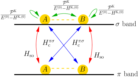
Figure 3: (Color online) Schematic diagram of the second order transition process generated by $H^{{\rm K},(2)}$ [Eq. (6)]. Pseudospin transitions (between the sublattices $A$ and $B$) and interband transitions (between $\pi$ and $\sigma$ bands) are illustrated.

Combined effects of the three factors $H_{\rm so}$, ${\cal P}^{\rm K}/(E^{(0)}-H^{\rm K,(0)})$, $H_{\rm c}$ are illustrated in Fig. 3. The real spin dependence arises solely from $H_{\rm so}$, which generates the factor $\sigma_{y}$ comment-sigma_y . For the pseudospin, the combined effect of $H_{\rm so}$ and $H_{\rm c}$ is to flip the pseudospin. When they are combined with the pseudospin conserving part of ${\cal P}^{\rm K}/(E^{(0)}\!-\!H^{\rm K,(0)})$, one obtains the pseudospin flipping process [Eq. (8)] determining $\delta_{\rm K}$. In addition, ${\cal P}^{\rm K}/(E^{(0)}\!-\!H^{\rm K,(0)})$ contains the pseudospin flipping part, which is natural since states localized in one particular sublattice are not eigenstates of $H^{\rm K,(0)}$. When the pseudospin flipping part of ${\cal P}^{\rm K}/(E^{(0)}-H^{\rm K,(0)})$ is combined with $H_{\rm so}$ and $H_{\rm c}$, one obtains the pseudospin conserving process [Eq. (8)] determining $\delta^{\prime}_{\rm K}$.

The signs of $\delta_{\rm K}e^{i\theta}$ and $\delta^{\prime}_{\rm K}/\cos 3\theta$ are negative. We find $|(\delta^{\prime}_{\rm K}/\cos 3\theta)/\delta_{\rm K}|=4.5$ for tight-binding parameters in Ref. Mintmire95Carbon . Thus $\delta^{\prime}_{\rm K}$ is of the same order as $\delta_{\rm K}$ parameters , which is understandable since pseudospin flipping terms in $E^{(0)}\!-\!H^{\rm{K},(0)}$ (with amplitudes $V_{pp}^{\sigma}$, $V_{sp}^{\sigma}$) are comparable in magnitude to pseudospin conserving terms (with amplitudes $E^{(0)}\!-\!\varepsilon_{s(p)}$).

IV Behavior in a magnetic field

Next we examine further implications of our result in view of the experiment Kuemmeth08Nature , where the conduction band bottom and valence band top positions of semiconducting CNTs ($\nu\!=\!\pm 1$) are measured as a function of the magnetic field $B$ parallel to the CNT axis. We find that the $\theta$ dependence [Eq. (3)] of $\delta^{\prime}_{\rm K}$ has interesting implications. When $\cos 3\theta$ is sufficiently close to $0$ (close to armchair-type), $|\delta^{\prime}_{\rm K}|$ is smaller than $|\delta_{\rm K}e^{i\theta}|$. The prediction of our theory in this situation is shown in Figs. 4(a) and (b). Note that the spin splitting of both the conduction and valence bands becomes smaller as the energy $E$ increases. On the other hand, when $\cos 3\theta$ is sufficiently close to $1$ (close to zigzag-type), $|\delta^{\prime}_{\rm K}|$ is larger than $|\delta_{\rm K}e^{i\theta}|$. In this situation [Figs. 4(c) and (d)], the energy dependence of either valence or conduction band is inverted; For $\nu\!=\!+1(-1)$, the spin splitting of the valence (conduction) band becomes larger as the the energy increases.

Combined with the electron-prevailing [Figs. 4(a) and (c) for $\nu\!=\!+1$] vs. hole-prevailing [Figs. 4(b) and (d) for $\nu\!=\!-1$] asymmetries in the zero-field splitting, one then finds that there exist four distinct patterns of $E$ vs. $B$ diagram, which is the second main result of this paper. Among these 4 patterns, only the pattern in Fig. 4(a) is observed in the experiment Kuemmeth08Nature , which measured two CNT samples. We propose further experiments to test the existence of the other three patterns.

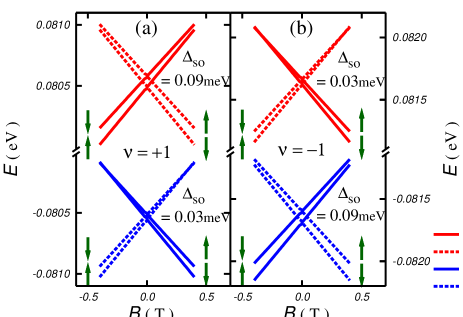
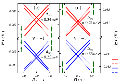
Figure 4: (Color online) Calculated energy spectrum of the conduction band bottom (red, $E>0$) and valence band top (blue, $E<0$) near K (solid lines) and K^′ (dashed lines) points in semiconducting CNTs with $R\!\approx\!2.5\,$nm as a function of magnetic field $B$ parallel to the CNT axis. The chiral vectors for each CNT are (a) (38,34), (b) (39,34), (c) (61,0), and (d) (62,0), respectively. Arrows (green) show spin direction along the CNT axis and $\Delta_{\rm so}$ denotes the zero-field splitting. Assuming $k_{y}\!=\!0$, the energy $E$ including the SOC, the Aharonov-Bohm flux Ajiki93JPSJ $\phi_{\rm AB}\!=\!{B\pi R^{2}}$, and the Zeeman coupling effects is, $E\!=\!\pm\hbar v_{F}\sqrt{(k_{x}\!+\!{(1/R)}{(\phi_{\rm AB}/\phi_{0})})^{2}}+E_{\uparrow(\downarrow)}^{{\rm K(K^{\prime})},(2)}\!+\!{(g/2)}\mu_{\rm B}\tau_{\|}B$, with upper (lower) sign applying to the conduction (valence) band. $\phi_{0}\!=\!{hc/|e|}$, $\tau_{\|}\!=\!+1(-1)$ for $\chi_{\uparrow(\downarrow)}$, $v_{F}\!=\!-aV_{pp}^{\pi}{\sqrt{3}/2}$, and $g\!=\!2$ Kuemmeth08Nature . For estimation of $E_{\uparrow(\downarrow)}^{{\rm K(K^{\prime})},(2)}$, we use tight-binding parameters in Ref. Mintmire95Carbon ; $V_{ss}^{\sigma}\!=\!-4.76\,$eV, $V_{sp}^{\sigma}\!=\!4.33\,$eV, $V_{pp}^{\sigma}\!=\!4.37\,$eV, $V_{pp}^{\pi}\!=\!-2.77\,$eV, $\varepsilon_{s}\!=\!-6.0\,$eV, and $\varepsilon_{p}\!=\!0$ parameters .

Here we remark that although Eqs. (1), (2), (3) are demonstrated so far for semiconducting CNTs, they hold for metallic CNTs ($\nu\!=\!0$) as well. For armchair CNTs with $\cos 3\theta\!=\!0$, $\delta^{\prime}_{\rm K}$ becomes zero and the spin splitting is determined purely by $\delta_{\rm K}$. For metallic but non-armchair CNTs, finding implications of Eq. (1) is somewhat technical since the curvature-induced minigap appears near the Fermi level Kane97PRL . Our calculation for $(37,34)(\cos 3\theta\!\approx\!0)$ and $(60,0)(\cos 3\theta\!=\!1)$ CNTs including the minigap effect indicates that they show behaviors similar to Fig. 4(b) and (d), respectively. Thus nominally metallic CNTs exhibit spin splitting patterns of $\nu\!=\!-1$ CNTs.

V Discussion and summary

Lastly we discuss briefly the effective SOC in a curved graphene Meyer07Nature . Unlike CNTs, there can be both convex-shaped and concave-shaped curvatures in a graphene. We first address the convex-shaped curvatures. When the local structure of a curved graphene has two principal curvatures, $1/R_{1}$ and $1/R_{2}$ with the corresponding binormal unit vectors ${\bf n}_{1}$ and ${\bf n}_{2}$, each principal curvature $1/R_{i}$ $(i\!=\!1,2)$ generates the effective SOC, Eq. (1), with $\sigma_{y}$ replaced by ${\bm{\sigma}}\cdot{{\bf n}_{i}}$ and $R$ by $R_{i}$. The corresponding $\delta_{i}$ and $\delta^{\prime}_{i}$ values are given by Eqs. (2) and (3) with $\theta$ replaced by $\theta_{i}$, where $\theta_{i}$ is the chiral angle with respect to ${\bf n}_{i}$. Thus the diagonal term of the effective SOC is again comparable in magnitude to the off-diagonal term. For the concave-shaped curvatures, we find that the two types of the SOC become $-\delta_{i}$ and $-\delta^{\prime}_{i}$ with $\theta_{i}$, respectively. We expect that this result may be relevant for the estimation of the spin relaxation length in graphenes Hernando08Condmat and may provide insights into unexplained experimental data in graphene-based spintronic systems Han09PRL . We also remark that the effective SOC in a graphene may be spatially inhomogeneous since the local curvature of the nanometer-scale corrugations Meyer07Nature is not homogeneous, whose implications go beyond the scope of this paper.

In summary, we have demonstrated that the interplay of the atomic SOC and the curvature generates two types of the effective SOC in a CNT, one of which was not recognized before. Combined effects of the two types of the SOC in CNTs explain recently observed electron-hole asymmetric spin splitting Kuemmeth08Nature and generates four qualitatively different types of energy level dependence on the parallel magnetic field. Our result may have interesting implications for graphenes as well.

Note added.– While we were preparing our manuscript, we became aware of a related paper Chico09PRB . However the effective Hamiltonian [Eq. (1)] for the SOC and the four distinct types of the magnetic field dependence (Fig. 4) are not reported in the work.

- (1) S. Sahoo, T. Kontos, J. Furer, C. Hoffmann, M. Gräber, A. Cuttet, and C. Schönenberger, Nat. Phys. 1, 99 (2005).
- (2) C. A. Merchant and N. Marković, Phys. Rev. Lett. 100, 156601 (2008).
- (3) N. Tombros, C. Jozsa, M. Popinciuc, H. T. Jonkman, and B. J. van Wees, Nature (London) 448, 571 (2007); S. Cho, Y.-F. Chen, and M. S. Fuhrer, Appl. Phys. Lett. 91, 123105 (2007).
- (4) K. Tsukagoshi, B. W. Alphenaar, and H. Ago, Nature (London) 401, 572 (1999).
- (5) D. V. Bulaev, B. Trauzettel, and D. Loss, Phys. Rev. B 77, 235301 (2008).
- (6) D. Huertas-Hernando, F. Guinea, and A. Brataas, arXiv:0812.1921 (unpublished).
- (7) H. Min, J. E. Hill, N. A. Sinitsyn, B. R. Sahu, L. Kleinman, and A. H. MacDonald, Phys. Rev. B 74, 165310 (2006); Y. Yao, F. Ye, X.-L. Qi, S.-C. Zhang, and Z. Fang, ibid. 75, 041401(R) (2007).
- (8) D. Huertas-Hernando, F. Guinea, and A. Brataas, Phys. Rev. B 74, 155426 (2006).
- (9) T. Ando, J. Phys. Soc. Jpn. 69, 1757 (2000); A. DeMartino, R. Egger, K. Hallberg, and C. A. Balseiro, Phys. Rev. Lett. 88, 206402 (2002).
- (10) J. C. Meyer, A. K. Geim, M. I. Katsnelson, K. S. Novoselov, T. J. Booth, and S. Roth, Nature (London) 446, 60 (2007); E. Stolyarova, K. T. Rim, S. Ryu, J. Maultzsch, P. Kim, L. E. Brus, T. F. Heinz, M. S. Hybertsen, and G. W. Flynn, Proc. Natl. Acad. Sci. U.S.A. 104, 9209 (2007); V. Geringer, M. Liebmann, T. Echtermeyer, S. Runte, M. Schmidt, R. Rückamp, M. C. Lemme, and M. Morgenstern, Phys. Rev. Lett. 102, 076102 (2009); A. K. Geim, Science 324, 1530 (2009).
- (11) V. M. Pereira and A. H. Castro Neto, Phys. Rev. Lett. 103, 046801 (2009).
- (12) F. Kuemmeth, S. Ilani, D. C. Ralph, and P. L. McEuen, Nature (London) 452, 448 (2008).
- (13) The corresponding expression in Ref. Hernando06PRB is slightly different from Eq. (2) since the band is treated in different ways. When a few minor mistakes in Ref. Hernando06PRB are corrected, the two expressions result in similar numerical values.
- (14) J. Serrano, M. Cardona, and T. Ruf, Solid State Commun. 113, 411 (2000).
- (15) J. Ajiki and T. Ando, J. Phys. Soc. Jpn. 62, 1255 (1993).
- (16) Leonard I. Schiff, Quantum Mechanics (McGraw-Hill, New York, 1968).
- (17) is spin-independent and thus ignored [see Eq. (III)].
- (18) For the point, , with upper (lower) sign for the conduction band bottom (valence band top).
- (19) J. C. Slater and G. F. Koster, Phys. Rev. 94, 1498 (1954).
- (20) The last four terms of in Eq. (9), which do not commute with , do not contribute to the effective SOC near the Fermi energy due to the factor Hernando06PRB .
- (21) J. W. Mintmire and C. T. White, Carbon 33, 893 (1995).
- (22) Using other sets of tight-binding parameters [D. Tománek and M. A. Schluter, Phys. Rev. Lett. 67, 2331 (1991); R. Saito, M. Fujita, G. Dresselhaus, and M. S. Dresselhaus, Phys. Rev. B 46, 1804 (1992)] does not change results qualitatively.
- (23) C. L. Kane and E. J. Mele, Phys. Rev. Lett. 78, 1932 (1997); L. Yang and J. Han, ibid. 85, 154 (2000); A. Kleiner and S. Eggert, Phys. Rev. B 63, 073408 (2001); J.-C. Charlier, X. Blase, and S. Roche, Rev. Mod. Phys. 79, 677 (2007).
- (24) See for instance, W. Han, W. H. Wang, K. Pi, K. M. McCreary, W. Bao, Y. Li, F. Miao, C. N. Lau, and R. K. Kawakami, Phys. Rev. Lett. 102, 137205 (2009).
- (25) L. Chico, M. P. López-Sancho, and M. C. Muñoz, Phys. Rev. B 79, 235423 (2009).