Open-system dynamics of graph-state entanglement

Abstract

We consider graph states of arbitrary number of particles undergoing generic decoherence. We present methods to obtain lower and upper bounds for the system’s entanglement in terms of that of considerably smaller subsystems. For an important class of noisy channels, namely the Pauli maps, these bounds coincide and thus provide the exact analytical expression for the entanglement evolution. All the results apply also to (mixed) graph-diagonal states, and hold true for any convex entanglement monotone. Since any state can be locally depolarized to some graph-diagonal state, our method provides a lower bound for the entanglement decay of any arbitrary state. Finally, this formalism also allows for the direct identification of the robustness under size scaling of graph states in the presence of decoherence, merely by inspection of their connectivities.

Introduction.– Graph states graph_review constitute an important class of entangled states with broad-reaching applications in quantum information, including measurement-based quantum computation Brie_review ; RausBrie , quantum error correction SchWer , and secure quantum communication DurCasBrie-ChenLo . Moreover, instances of this family, such as the Greenberger-Horne-Zeilinger states, play a crucial role in fundamental tests of quantum non-locality GHZ . Consequently, a great effort has been made both to theoretically understand their properties graph_review ; HeinEisBrie and to create and coherently manipulate them experimentally ClusterExp

Needless to say, it is crucial to understand the dynamics of their entanglement in realistic scenarios, where the system unavoidably decoheres due to experimental errors or to the interaction with its environment. Previous studies on the robustness of graph-state entanglement in the presence of decoherence observed a disentanglement time (or lower bounds thereof) insensitive to the system size Simon&Kempe ; HeinDurBrie . However, the disentanglement time on its own is not in general able to provide any faithful assessment about the entanglement’s robustness, since it can grow with the number $N$ of particles and yet the entanglement can get closer to zero the faster, the larger $N$ us . The full dynamical evolution of entanglement must then be studied to draw conclusions on its fragility. Taking the latter into account, the entanglement of the linear-cluster states, an example of graph states, was shown to be robust with the size of the system against the particular case of collective dephasing decoherence Guhne .

The present work provides a general framework for the study of the entanglement evolution of graph states under decoherence. Our techniques apply to (i) any graph, and graph-diagonal, states; (ii) arbitrary kinds of noise, individual or collective; and (iii) any convex (bi- or multi-partite) entanglement quantifier that does not increase under local operations and classical communication (LOCC). In the developed formalism we consider local measurement protocols to efficiently obtain lower and upper bounds for the entanglement of the whole system contained in any given partition in terms of that of a considerably smaller subsystem consisting only of those qubits lying on the boundary of the partition. No optimization on the full system’s parameter space is required throughout. For an important class of noisy channels – namely arbitrary Pauli maps, to be defined below – the lower and upper bounds coincide, providing thus the exact entanglement evolution. With the same methods we also establish a second family of lower bounds that, despite less tight, depend only on the connectivity of the graph and not on its size. This allows us to assess the robustness based on the full dynamics of the entanglement and not just its disentanglement time. Our approach can also be used to establish lower bounds to the entanglement behavior of any initial quantum state.

Graph states.– Consider a mathematical graph $G_{(\mathcal{V},\mathcal{E})}\equiv\{\mathcal{V},\mathcal{E}\}$, composed of a set $\mathcal{V}$, of $N$ vertices $i\in\mathcal{V}$, and a set $\mathcal{E}$, of edges $\{i,j\}\in\mathcal{E}$ connecting each vertex $i$ to some other $j$. The associated physical state is operationally defined as follows: to each vertex $i$ associate a qubit, initialize all $N$ qubits in the product state $|{g_{(\mathcal{V})}}_{0}\rangle\equiv\bigotimes_{i\in\mathcal{V}}|+_{i}\rangle$, being $|+_{i}\rangle=(|0_{i}\rangle+|1_{i}\rangle)/\sqrt{2}$, and to all pairs $\{i,j\}$ of qubits joined by an edge apply a maximally-entangling control-$Z$ ($CZ$) gate, $CZ_{ij}=|0_{i}0_{j}\rangle\langle 0_{i}0_{j}|+|0_{i}1_{j}\rangle\langle 0_{i}1_{j}|+|1_{i}0_{j}\rangle\langle 1_{i}0_{j}|-|1_{i}1_{j}\rangle\langle 1_{i}1_{j}|$. The resulting $N$-qubit graph state is

$$|{G_{(\mathcal{V},\mathcal{E})}}_{0}\rangle=\bigotimes_{\{i,j\}\in\mathcal{E}}CZ_{ij}|{g_{(\mathcal{V})}}_{0}\rangle.$$ (1)

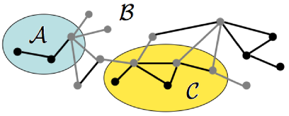
Figure 1: (Color online) Example of a mathematical graph associated to a physical graph state. We have displayed a possible partition of this graph, splitting the system in three parts $\mathcal{A}$, $\mathcal{B}$, and $\mathcal{C}$. The vertices and edges in grey corresponds to the boundary qubits and the boundary-crossing edges respectively.

An example of such graph is shown in Fig. 1, where the system is divided into three regions, $\mathcal{A}$, $\mathcal{B}$ and $\mathcal{C}$. We call all edges that go from one region to the other the boundary-crossing edges and label the subset of all such edges by $\mathcal{X}$. All qubits connected by the boundary-crossing edges are in turn called the boundary qubits and the subset composed of all of these is called $\mathcal{Y}$.

Open-system dynamics.– Our ultimate goal is to quantify the entanglement in any partition of arbitrary graph states undergoing a generic physical process during a time interval $t$. The action of such process on an initial density operator $\rho$ can be described by a completely-positive trace-preserving map $\Lambda$ as $\rho_{t}=\Lambda(\rho)$, where $\rho_{t}$ is the evolved density matrix after time $t$. All such maps can be expressed in a Kraus representation, $\Lambda(\rho)=\sum_{\mu}p_{\mu}K_{\mu}\rho K_{\mu}^{\dagger}$, where $\sqrt{p_{\mu}}K_{\mu}$ are called the Kraus operators (each of which appearing with probability $p_{\mu}$), which satisfy the normalization conditions Tr$[K_{\mu}^{\dagger}K_{\mu}]=1$ and $\sum_{\mu}p_{\mu}=1$ nielsen . The Kraus representation guarantees that the map is (completely) positive and preserves trace normalization. When the map can be factorized as the composition of individual maps acting independently on each qubit, the noise is said to be individual (or independent); if not, it is said to be collective.

A very important class of processes is described by the Pauli maps, separable (non-entangling) maps whose Kraus operators are given by tensor products of Pauli operators $X$, $Y$, $Z$, and the identity. Examples of these are the collective or individual depolarizing, dephasing or bit-flip channels nielsen . As we show next, it is possible to determine the exact entanglement evolution of graph and graph-diagonal states (whose formal definition is provided below) subject to individual Pauli maps.

Exact entanglement of graph states under Pauli maps.–

Let us start by recalling that a graph state is the simultaneous eigenvector – of eigenvalue 1 – of the $N$ generators of the stabilizer group, that is, of the $N$ operators consisting each of which of one $X$ acting on each single qubit and $Z$’s on all its neighboring ones graph_review . Therefore, the application of an $X$ or $Y$ operator on a qubit $k$ of a graph state is equivalent to the application of $Z$ operators on all neighboring qubits of $k$, or on all of its neighboring qubits and on $k$ itself, respectively. The action of any Pauli map $\Lambda$ on a graph state is thus equivalent to that of another separable map, $\tilde{\Lambda}$, whose Kraus operators $\tilde{K}_{\mu}$ are obtained from $K_{\mu}$ replacing in the latter each $X$ and $Y$ operators by tensor products of $Z$ and identity operators according to the rule just described comment . Thus we need to consider how a general combination of $Z$ operators acts on a graph state. We use the multi-index $\tilde{\mu}=(\mu_{1},...,\mu_{N})$, with $\mu_{i}=\{0,1\}$, to denote such a combination through $Z^{\mu_{1}}\otimes Z^{\mu_{2}}\otimes...\otimes Z^{\mu_{N}}$. The action of such operator on a graph state $|{G_{(\mathcal{V},\mathcal{E})}}_{0}\rangle$ generates another graph state $|{G_{(\mathcal{V},\mathcal{E})}}_{\tilde{\mu}}\rangle$, orthogonal to the former one graph_review ; HeinDurBrie . These considerations imply that $\rho_{t}$ can be expressed as

$$\rho_{t} = \Lambda(|{G_{(\mathcal{V},\mathcal{E})}}_{0}\rangle)=\tilde{\Lambda}(|{G_{(\mathcal{V},\mathcal{E})}}_{0}\rangle)$$ (2)

$$= \sum_{\tilde{\mu}}\tilde{p}_{\tilde{\mu}}|{G_{(\mathcal{V},\mathcal{E})}}_{\tilde{\mu}}\rangle\langle{G_{(\mathcal{V},\mathcal{E})}}_{\tilde{\mu}}|.$$

All possible $2^{N}$ graph states $|{G_{(\mathcal{V},\mathcal{E})}}_{\tilde{\mu}}\rangle$ associated to the graph $G_{(\mathcal{V},\mathcal{E})}$ form a complete orthonormal basis of the $N$-qubit Hilbert space. State (2) is a graph-diagonal state. Calculating the exact entanglement in any partition of the such state is in general a problem that involves an optimization over the entire parameter space of $\rho_{t}$. In what follows we will show that it is possible to greatly reduce the complexity of this optimization problem. Consider any partition of the state $\rho_{t}$. We now factor out explicitly all the $CZ$ gates but those corresponding to the boundary-crossing edges and write the state as

$$\rho_{t} = \bigotimes_{\{i,j\}\in\mathcal{E}/\mathcal{X}}CZ_{ij}\sum_{\gamma,\delta}\tilde{p}_{\gamma,\delta}|{G_{(\mathcal{Y},\mathcal{X})}}_{\gamma}\rangle\langle{G_{(\mathcal{Y},\mathcal{X})}}_{\gamma}|$$ (3)

$$\otimes |{g_{(\mathcal{V}/\mathcal{Y})}}_{\delta}\rangle\langle{g_{(\mathcal{V}/\mathcal{Y})}}_{\delta}|\bigotimes_{\{k,l\}\in\mathcal{E}/\mathcal{X}}CZ_{kl},$$

Here we have grouped together all indices inside $\tilde{\mu}$ into two new multiple indices, $\gamma$ and $\delta$. Multiple index $\gamma$ accounts for all possible graph states $|{G_{(\mathcal{Y},\mathcal{X})}}_{\gamma}\rangle$ generated by applying tensor products of $Z$ and identity operators to the graph state $|{G_{(\mathcal{Y},\mathcal{X})}}_{0}\rangle\equiv\bigotimes_{\{i,j\}\in\mathcal{X}}CZ_{ij}\otimes|{g_{(\mathcal{Y})}}_{0}\rangle$, associated to the boundary graph $G_{(\mathcal{Y},\mathcal{X})}=\{\mathcal{Y},\mathcal{X}\}$, with $|{g_{(\mathcal{Y})}}_{0}\rangle\equiv\bigotimes_{i\in\mathcal{Y}}|+_{i}\rangle$. Multiple index $\delta$ on the other hand accounts for all states $|{g_{(\mathcal{V}/\mathcal{Y})}}_{\delta}\rangle$ generated from $Z$ or identity operators on the state $|{g_{(\mathcal{V}/\mathcal{Y})}}_{0}\rangle\equiv\bigotimes_{i\in\mathcal{V}/\mathcal{Y}}|+_{i}\rangle$ of the non-boundary qubits $\mathcal{V}/\mathcal{Y}$. Probability $\tilde{p}_{\gamma,\delta}$ is defined as the sum of all $p_{\mu}$ such that $\tilde{K}_{\mu}|{G_{(\mathcal{Y},\mathcal{X})}}_{0}\rangle\otimes|{g_{(\mathcal{V}/\mathcal{Y})}}_{0}\rangle=|{G_{(\mathcal{Y},\mathcal{X})}}_{\gamma}\rangle\otimes|{g_{(\mathcal{V}/\mathcal{Y})}}_{\delta}\rangle$. Because the $CZ$ gates explicitly factored out in state (3) are local unitary operations with respect to the partition of interest, the entanglement of $\rho_{t}$, $E(\rho_{t})$, reads

$$E\big{(}\sum_{\gamma,\delta}\tilde{p}_{\gamma,\delta}|{G_{(\mathcal{Y},\mathcal{X})}}_{\gamma}\rangle\langle{G_{(\mathcal{Y},\mathcal{X})}}_{\gamma}|\otimes|{g_{(\mathcal{V}/\mathcal{Y})}}_{\delta}\rangle\langle{g_{(\mathcal{V}/\mathcal{Y})}}_{\delta}|\big{)}.$$ (4)

where $E$ is any convex entanglement quantifier not increasing under LOCC. In what follows, we first establish a lower and upper bound to this expression and then show that these bounds coincide, obtaining the exact expression of the graph-state entanglement evolution.

First, consider an LOCC protocol consisting of measuring all the non-boundary qubits $\mathcal{V}/\mathcal{Y}$ of the state within brackets in Eq. (4) in the product basis composed by all orthonormal states $\{|{g_{(\mathcal{V}/\mathcal{Y})}}_{\delta}\rangle\}$ and tracing out the measured subsystem after communicating the outcomes. The remaining subsystem $\mathcal{Y}$ is flagged by each measurement outcome $\delta$ – meaning that outcome $\delta$ provides full information about to which state $\mathcal{Y}$ has been projected after each measurement run. The final entanglement after the entire protocol is then given by the average entanglement over all measurement runs. Since $E$ is non-increasing under LOCC, $E(\rho_{t})$ must satisfy

$$E(\rho_{t})\geq\sum_{\delta}\tilde{p}_{\delta}E\Big{(}\sum_{\gamma}\tilde{p}_{(\gamma|\delta)}|{G_{(\mathcal{Y},\mathcal{X})}}_{\gamma}\rangle\langle{G_{(\mathcal{Y},\mathcal{X})}}_{\gamma}|\Big{)},$$ (5)

where $\tilde{p}_{\delta}\equiv\sum_{\gamma}\tilde{p}_{\gamma,\delta}$ is the total probability of occurrence of an event $\delta$ and $\tilde{p}_{(\gamma|\delta)}$ is the conditional probability of an event $\gamma$ given that event $\delta$ has happened.

On the other hand, convexity of $E$ implies that $E(\rho_{t})$, as given by (4), must necessarily be smaller or equal to $\sum_{\delta}\tilde{p}_{\delta}E\Big{(}\sum_{\gamma}\tilde{p}_{(\gamma|\delta)}|{G_{(\mathcal{Y},\mathcal{X})}}_{\gamma}\rangle\langle{G_{(\mathcal{Y},\mathcal{X})}}_{\gamma}|\otimes|{g_{(\mathcal{V}/\mathcal{Y})}}_{\delta}\rangle\langle{g_{(\mathcal{V}/\mathcal{Y})}}_{\delta}|\Big{)}$, which, since locally added ancillary systems do not change the entanglement, is in turn equal to the right-hand side of (5). This means that the right-hand side of Eq. (5) provides at the same time an upper and a lower bound to $E(\rho_{t})$ and therefore yields its exact value, i.e. :

$$E(\rho_{t})=\sum_{\delta}\tilde{p}_{\delta}E\Big{(}\sum_{\gamma}\tilde{p}_{(\gamma|\delta)}|{G_{(\mathcal{Y},\mathcal{X})}}_{\gamma}\rangle\langle{G_{(\mathcal{Y},\mathcal{X})}}_{\gamma}|\Big{)}.$$ (6)

A comment on the implications of this exact result on the computational-cost is now in place. The calculation of the entanglement of systems composed by $N=N_{\mathcal{Y}}+N_{\mathcal{V}/\mathcal{Y}}$ qubits (being $N_{\mathcal{Y}}$ and $N_{\mathcal{V}/\mathcal{Y}}$ the number of boundary and non-boundary qubits respectively) is a problem that, in general, involves an optimization over $O\big{(}2^{2N}\big{)}$ real parameters. Through Eq. (6) such calculation is reduced to that of the average entanglement over a sample of $2^{N_{\mathcal{V}/\mathcal{Y}}}$ states (one for each measurement outcome $\delta$) of $N_{\mathcal{Y}}$ qubits, which involves at most $2^{N_{\mathcal{V}/\mathcal{Y}}}$ optimizations over $O\big{(}2^{2N_{\mathcal{Y}}}\big{)}$ real parameters. Thus the present method provides an exponential decrease in the computational power needed to calculate $E(\rho_{t})$, since only the boundary qubits appear in the computation of Eq. (6).

In order to illustrate the power of the method we have calculated, using (6), the exact entanglement of formation $E_{F}$ Wootters of 1-D graph states under the action of independent depolarizing channels, which mix, with probability $p$, any one-qubit state with the maximally mixed state $\openone/2$  nielsen . In Fig. 2 we display the curves corresponding to the bipartition first qubit versus the rest, although other partitions can be considered. The 1-D graph state (also called the linear cluster state), given by $|LC\rangle=\bigotimes_{i=1}^{N-1}CZ_{i,i+1}\bigotimes_{k}^{N}|+_{k}\rangle$, evolves from $p=0$ towards a final maximally mixed state at $p=1$. Not only this calculation would have been impossible had we attempted a brute-force optimization approach, but also, since in this particular case the boundary qubits are just two, the use of (6) allows to perform the calculation with no optimization at all, for an explicit formula for the entanglement of formation exists for arbitrary two-qubit systems Wootters .

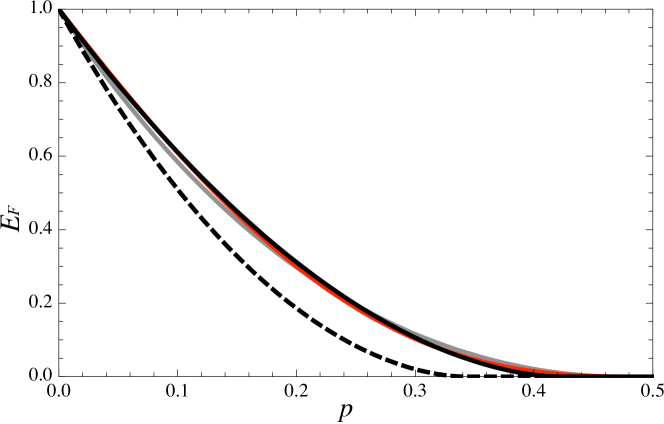
Figure 2: (Color online.) Entanglement of formation ($E_{F}$) in the partition of the first particle versus the rest for 1-D graph states of 2 (black), 4 (grey) and 7 (red) particles undergoing individual depolarization as a function of the depolarization probability $p$. The dashed curve represents a size-independent lower bound.

Beyond graph states and Pauli maps.– The expression (6) is actually a method for calculating the entanglement of any graph-diagonal state as the one in (2). Since Pauli maps acting on initial graph-diagonal states also produce graph-diagonal states, all the arguments used so far are also valid for this class of initial states. Furthermore, any quantum state can be depolarized to a graph-diagonal state by means of LOCC ADB . Using again the fact that the entanglement of a state does not increase if an LOCC protocol is applied, one can see that the present method also provides (in general non-tight) lower bounds to the decay of the entanglement of any initial state subject to any decoherence process.

Robustness of graph-state entanglement.– The developed techniques can be further simplified to obtain new lower bounds to graph-state entanglement during all the evolution that, despite not being tight, can be calculated in a much more efficient way than (5) and often turn out to be independent of the total number of qubits. This dramatically simplifies the study of the entanglement robustness of graph states as a function of the system’s size, a central question for the applicability of these states as quantum information resources. As an illustration, we compare next graph states of different sizes under the action of general $N$-qubit Pauli maps $\Lambda$ that scale with $N$ in a way such that, for each $\sqrt{p_{\mu}}K_{\mu}$, the Kraus operators of the map acting on $M$ more qubits are obtained as tensor products of $\sqrt{p_{\mu}}K_{\mu}$ with Pauli or identity operators on the other $M$ qubits, weighted with some new probabilities that sum up to one (for each $\mu$). That is, so that the total probability of event $\mu$ on the $N$ first qubits, $p_{\mu}$, remains the same. All the individual or collective Pauli maps mentioned above fall into this category. The state between brakets in Eq. (4) can then be written also as $\sum_{\gamma}\tilde{p}_{\gamma}|{G_{(\mathcal{Y},\mathcal{X})}}_{\gamma}\rangle\langle{G_{(\mathcal{Y},\mathcal{X})}}_{\gamma}|\otimes\sum_{\delta}\tilde{p}_{(\delta|\gamma)}|{g_{(\mathcal{V}/\mathcal{Y})}}_{\delta}\rangle\langle{g_{(\mathcal{V}/\mathcal{Y})}}_{\delta}|\big{)}$, where $\tilde{p}_{\gamma}\equiv\sum_{\delta}\tilde{p}_{\gamma,\delta}$ and $\tilde{p}_{(\delta|\gamma)}$ is the conditional probability of $\delta$ given $\gamma$. By tracing out the state of the non-boundary qubits (i.e., by disregarding the flag that lead to (5) above) and using again the fact that $E$ does not increase under LOCC, we arrive at

$$E(\rho_{t})\geq E\big{(}\sum_{\gamma}\tilde{p}_{\gamma}|{G_{(\mathcal{Y},\mathcal{X})}}_{\gamma}\rangle\langle{G_{(\mathcal{Y},\mathcal{X})}}_{\gamma}|\big{)}.$$ (7)

Now, notice that – for the maps here-considered – probability $\tilde{p}_{\gamma}$ depends only on the boundary graph $G_{(\mathcal{Y},\mathcal{X})}$ and the number of non-boundary qubits directly connected to it (the boundary graph is affected by the noise on up to its first neighbors), not on the total system size $N$. Bound (7) is unaffected by the addition of $M$ extra particles if these new particles are not connected to the boundary subsystem. In the latter sense, and for the considered noise scenario, noisy graph-state entanglement is thus robust with respect to the variation of the system size provided $G_{(\mathcal{Y},\mathcal{X})}$ and its connectivity to the rest do not vary.

Size-independent bound (7) (for the case of $E=E_{F}$) is compared with the exact entanglement, again for a linear cluster and the individual depolarizing channel, in Fig. 2

Discussion.– To summarize, in this work we have presented a general framework to study the entanglement decay of graph states under decoherence. It is important to emphasize that any function that satisfies the requirements of convexity and monotonicity under LOCC falls into the range of applicability of the machinery here-developed. This includes genuine multipartite entanglement quantifiers, as well as those functions aiming at quantifying the usefulness of quantum states for given quantum informational tasks.

To conclude with, let us make the following observations. First, the techniques developed to obtain perfect bounds can also be applied to tackle some cases other than Pauli maps. For example, for graph states in the presence of individual thermal baths at arbitrary temperature, an LOCC procedure similar to the one used to obtain the bound (5), but using general measurements instead of orthogonal ones, can be used to obtain highly non-trivial entanglement lower bounds.

Second, bound (7), when restricted to bipartite entanglement, provides the same type of lower bound as the one used in section V-B of Ref. HeinDurBrie to find lower bounds to the entanglement lifetime for the case of $E$ being the negativity. The present bound has the advantage of dealing with other possible partitions and general entanglement quantifiers. All these topics will be touched upon elsewhere.

- (1) M. Hein et al., arXiv:quant-ph/0602096.
- (2) H. J. Briegel, D. E. Browne, W. D r, R. Raussendorf, and M. Van den Nest, Nature Phys. 5, 19 (2009).
- (3) R. Raussendorf and H. J. Briegel, Phys. Rev. Lett. 86, 5188 (2001); R. Raussendorf, D. E. Browne, and H. J. Briegel, Phys. Rev. A 68, 022312 (2003).
- (4) D. Schlingemann and R. F. Werner, Phys. Rev. A 65, 012308 (2001).
- (5) W. Dür, J. Calsamiglia, and H. J. Briegel, Phys. Rev. A 71, 042336 (2005); K. Chen, H.-K. Lo, Quant. Inf. and Comp. Vol.7, No.8 689 (2007).
- (6) D. M. Greenberger, M. A. Horne and A. Zeilinger, in Bell’s Theorem, Quantum Theory, and Conceptions of the Universe, M. Kafatos (Ed.), Kluwer, Dordrecht, 69 (1989).
- (7) M. Hein, J. Eisert, and H. J. Briegel, Phys. Rev. A 69, 062311 (2004).
- (8) P. Walther et al., Nature 434, 169 (2005); N. Kiesel et al., Phys. Rev. Lett. 95, 210502 (2005); C. Y-. Lu et al., Nature Phys. 3, 91 (2007); K. Chen et al., Phys. Rev. Lett. 99,120503 (2007); G. Vallone, E. Pomarico, F. De Martini, and P. Mataloni, Phys. Rev. Lett. 100, 160502 (2008).
- (9) C. Simon and J. Kempe, Phys. Rev. A 65, 052327 (2002).
- (10) W. Dür and H.-J Briegel, Phys. Rev. Lett. 92, 180403 (2004); M. Hein, W. Dür, H.-J. Briegel, Phys. Rev. A 71, 032350 (2005).
- (11) L. Aolita, R. Chaves, D. Cavalcanti, A. Acín, and L. Davidovich, Phys. Rev. Lett. 100, 080501 (2008); L. Aolita et al., Phys. Rev. A 79, 032322 (2009).
- (12) O. Gühne, F. Bodoky, and M. Blaauboer, Phys. Rev. A 78, 060301 (2008).
- (13) M. A. Nielsen, I. L. Chuang, Quantum Computation and Quantum Information (Cambridge Univ. Press, Cambridge, 2000).
- (14) H. Aschauer, W. Dür, H. -J. Briegel, Phys. Rev. A 71, 012319 (2005).
- (15) Notice that different indices can often lead to the same operator (the same product of operators).
- (16) W. K. Wootters, Phys. Rev. Lett. 80, 2245 (1998).