Molecular clouds and clumps in the Boston University–Five College Radio Astronomy Observatory Galactic Ring Survey

Abstract

The Boston University–Five College Radio Astronomy Observatory  (BU-FCRAO) Galactic Ring Survey  (GRS) of ¹³CO $J=1\rightarrow 0$  emission covers Galactic longitudes 18$\arcdeg<\ell<55.7\arcdeg$ and Galactic latitudes $|b|\leq 1\arcdeg$. Using the SEQUOIA array on the FCRAO 14m telescope, the GRS fully sampled the ¹³CO  Galactic emission (46″  angular resolution on a 22″  grid) and achieved a spectral resolution of 0.21 km s^-1. Because the GRS uses ¹³CO, an optically thin tracer, rather than ¹²CO, an optically thick tracer, the GRS allows a much better determination of column density and also a cleaner separation of velocity components along a line of sight. With this homogeneous, fully-sampled survey of ¹³CO  emission, we have identified 829 molecular clouds and 6124 clumps throughout the inner Galaxy using the CLUMPFIND algorithm. Here we present details of the catalog and a preliminary analysis of the properties of the molecular clouds and their clumps. Moreover, we compare clouds inside and outside of the 5 kpc ring and find that clouds within the ring typically have warmer temperatures, higher column densities, larger areas, and more clumps compared to clouds located outside the ring. This is expected if these clouds are actively forming stars. This catalog provides a useful tool for the study of molecular clouds and their embedded young stellar objects.

1 Introduction

The Boston University–Five College Radio Astronomy Observatory  (BU–FCRAO) Galactic Ring Survey  (GRS) is a survey of Galactic ¹³CO $J=1\rightarrow 0$  emission toward the first Galactic quadrant (Jackson et al., 2006). One of the primary goals of the GRS was the study the Milky Way’s so-called 5 kpc molecular ring. Discovered as a peak in the radial Galactic CO distribution midway between the sun and the Galactic center (Burton, 1976; Scoville & Solomon, 1975), the 5 kpc molecular ring contains $\sim$ 70%  of the molecular material within the solar circle (M $\sim$ 2 $\times$ 10⁹ $M_{\odot}$; Combes, 1991). It is the prominent feature in molecular maps of the Galaxy and is the location of the majority of Galactic star formation (Burton, 1976; Robinson et al., 1984; Clemens et al., 1988).

Because the 5 kpc ring covers such a large region of sky, a large, high angular resolution, sensitive survey is required to reveal the molecular clouds and dense clumps where star formation occurs. In order to be able to study their properties, the BU–FCRAO GRS was designed to map the ¹³CO  molecular line emission over a large portion of the 5 kpc ring and, in doing so, answer a number of fundamental questions that remain about the 5 kpc ring. For instance, how many molecular clouds does the 5 kpc ring contain? What are their properties? Do molecular clouds in the star-forming ring differ from clouds elsewhere in the Galaxy?

The GRS provides a unique database to identify star-forming molecular clouds and their dense clumps. The first step in such studies is to isolate, identify, and catalog the molecular clouds and their clumps. Combined with distance determinations, this catalog can characterize the cloud masses, sizes, line widths, and densities in a range of Galactic environments. This paper describes a catalog of molecular clouds and clumps identified using ¹³CO  data from the GRS which provides a new, homogeneous database for the study of the large- and small-scale structure of molecular gas throughout the inner Milky Way (e.g., Simon et al., 2001). The complete catalog is available in electronic form. In total, we identify 829 clouds and 6124 clumps. A preliminary analysis of their general characteristics is also presented. In particular, we compare the properties of those clouds located inside the 5 kpc molecular ring to those outside the ring.

2 The BU–FCRAO Galactic Ring Survey

The BU–FCRAO GRS (Jackson et al., 2006) mapped Galactic ¹³CO $J=1\rightarrow 0$  emission using the SEQUOIA multi-pixel array on the FCRAO 14 m telescope. The survey extended in Galactic longitude from $\ell=$ 18$\arcdeg$ to 55.7$\arcdeg$ and in Galactic latitude from $|b|\leq 1\arcdeg$, for a total of 75.4 square degrees. The survey’s velocity coverage was $-$5 to 135 km s^-1  for Galactic longitudes $\ell\leq 40\arcdeg$ and $-$5 to 85 km s^-1  for Galactic longitudes $\ell>40\arcdeg$. The typical rms sensitivity was $\sigma$(T${}_{A}^{*}$) $\sim$ 0.13 K. The survey comprises a total of 1,993,522 spectra. The data are available to the community at www.bu.edu/galacticring or in DVD form by request.

Unlike most previous surveys of the inner Galaxy, the GRS is fully sampled (46″  angular resolution on a 22″  grid), has a high spectral resolution (0.21 km s^-1), and traces ¹³CO $J=1\rightarrow 0$  emission. Compared to ¹²CO, the ¹³CO  molecule is $\sim$ 50 times less abundant and, thus, has a much lower optical depth. As a result, ¹³CO  is a much better tracer of column density. Moreover, because it suffers less from line blending and self-absorption, it can separate clouds along the same line of sight more easily than ¹²CO. Because of these improvements over previous surveys the GRS can detect many new structures and cloud cores previously missed by older ¹²CO  surveys (e.g., Sanders et al., 1986; Dame et al., 2001).

For more details of the telescope and instrumental parameters, the observing modes, the data reduction processes, and the emission and noise characteristics of the dataset see Jackson et al. (2006).

3 Identifying molecular clouds and clumps

We use the automated algorithm CLUMPFIND (Williams et al., 1994) to identify molecular clouds and clumps within the GRS. CLUMPFIND searches through a three-dimensional ($\ell$, $b$, $v$) data cube using iso-brightness surfaces to identify contiguous emission features without assuming an a priori shape. In this respect, it is more flexible than other cloud identification algorithms that artifically decompose the emission features into three-dimensional Gaussian profiles (e.g., GAUSSCLUMPS).

CLUMPFIND begins the search for clouds at the voxel with the peak brightness in the data cube. The algorithm steps down from this peak brightness in levels referred to as ‘contour increments’. During the first iteration the algorithm finds all contiguous voxels with brightnesses between the peak value and the next level (defined as the peak value minus the contour increment). If these contiguous voxels are isolated they are assigned to a new cloud. If they are contiguous with a previously identified cloud then they are assigned to that pre-existing cloud. The algorithm iterates until it reaches a minimum brightness level. At this lowest level, CLUMPFIND does not search for new clouds, but instead adds all emission at that level into pre-existing clouds. This procedure is straightforward for isolated emission peaks, but complicated for blended emission features. For blended emission, features are separated based on a ‘friends-of-friends’ algorithm (see Williams et al., 1994 for more details).

For each cloud (or clump) that is identified, CLUMPFIND gives the position of the peak of the emission for the cloud in ($\ell$, $b$, $v$), the peak temperature, the FWHM extent of the cloud in ($\ell$, $b$, $v$), an estimate of the radius of the cloud (assuming the total number of voxels form a sphere), the total number of voxels, and the sum of the emission within the voxels. Moreover, a three-dimensional ($\ell$, $b$, $v$) data cube is also created which is identical to the input data cube in ($\ell$, $b$, $v$) space. In this output cube, however, the temperature scale in each voxel is replaced by an integer which corresponds to the cloud to which it is assigned. This output cube is extremely useful for identifying the exact voxels associated with each individual cloud and is used extensively in the analysis described below.

3.1 Clouds

Giant molecular clouds (GMCs) are generally defined as extended molecular line emission features with typical properties as outlined in Table 1. Molecular clouds do not have uniform densities, but are observed to be fragmented on all size scales. We refer to the dense regions within GMCs where clusters may form as ‘clumps’ and the smaller, denser sites where the individual star formation occurs as ‘cores’. Table 1 compares the typical properties of each of these structures.

3.1.1 Smoothing of the GRS data

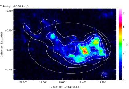
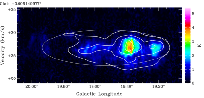
Figure 1: An example of the comparison between the full angular and spectral resolution GRS data (in color scale) and the smoothed data (as contours) for GRSMC G019.39$-$00.01. The top panel shows a single ($\ell,b$)  channel while the lower panel shows a single plane in ($\ell,v$)  space. The smoothed data were generated by smoothing both spatially (6′  on a 3′  grid) and spectrally (0.6 km s^-1) the original data. The smoothed data have an rms sensitivity of $\sigma$(T${}_{A}^{*}$) $\sim$ 0.01 K. The contour levels are 0.2 to 3.0 K in steps of 0.3 K on the ($\ell,b$)  image and 0.2 to 2.0 in steps of 0.4 K in the ($\ell,v$)  image. The white ellipses mark the approximate extent of the cloud in ($\ell,b$)  and ($\ell,v$)  space.

To improve the signal-to-noise and to better identify faint, extended molecular clouds we smoothed the GRS data both spatially (to a resolution of 6′) and spectrally (to a resolution of 0.6 km s^-1) using Gaussian kernels. Because this smoothing was moderate, it did not cause a significant loss of information in $\ell$, $b$, or $v$. In particular, this smoothing did not cause molecular clouds to be artifically blended along the line-of-sight. The smoothing improved the rms sensitivity from $\sim$0.13 K for the original data to $\sim$ 0.01 K for the smoothed data. The smoothed data were then re-sampled on a 3′  grid. Figure 1 shows a comparison between the original and smoothed data in both ($\ell,b$)  and ($\ell,v$)  space.

3.1.2 Modification of the CLUMPFIND algorithm

The CLUMPFIND algorithm was originally designed to identify the clumpy substructure within individual molecular clouds. To run CLUMPFIND, the user must specify two input parameters; the contour increment and the lowest brightness level. In the original algorithm, the lowest brightness level is hardwired to be a multiple of the contour increments which are forced to be evenly spaced, from the peak brightness to the minimum level. Because of the large dynamic range of the GRS data, however, the algorithm in this original form was unable to identify simultaneously both extended, diffuse clouds as well as compact, bright clouds. Moreover, it could not easily separate clouds that appeared distinct, especially at the lowest emission levels. For instance, by specifying a large contour increment (e.g. 0.7 K) CLUMPFIND would identify the brightest clouds in the GRS as one contiguous feature, but missed or merged many of the fainter, more extended clouds. However, with a smaller contour increment (e.g. 0.1 K), CLUMPFIND would better identify and separate the fainter, extended clouds, but the largest, brightest clouds would be artificially dissected and identified as numerous separate clouds.

Thus, in order to identify molecular clouds within the GRS at all emission levels, we modified the CLUMPFIND algorithm. For this purpose we required a large contour increment, but a small minimum brightness level. To achieve this, we changed the minimum brightness level to be a user input variable independent of the contour increment. In this scheme, we retained evenly spaced contour levels between the peak and minimum brightness levels as per the original algorithm but could additionally search for clouds to a lower brightness level. This scheme allowed us to identify both faint, extended clouds and bright, compact clouds with the same input parameters.

3.1.3 Selection of CLUMPFIND input parameters

With this modified version of CLUMPFIND, we tested a range of contour increments and lowest brightness levels to determine which set of parameters would best identify molecular clouds. Because of the inherent difficulties in determining where one cloud ends and the next begins, different choices of these parameters will certainly result in different output catalogs. However, regardless of the exact parameters, the bright, large molecular clouds are typically always recovered; the differences in the catalogs is most noticeable in the separation of nearby emission features and for the faint, small clouds.

To test the performance of the algorithm we completed a series of simple tests to compare the clouds identified with CLUMPFIND to the original dataset. In essence we replaced the CLUMPFIND clouds with elliptical three-dimensional Gaussian models with the same peak temperature, center position, size, orientation, line width and voxels of each cloud identified by CLUMPFIND. We then subtracted these Gaussian models from the original dataset and examined the residuals. We describe this process below.

We ran three representative regions within the smoothed GRS (each covering $\Delta\ell\times\Delta b$ = 2^∘$\times$2^∘) through CLUMPFIND, varying both the contour increment and the minimum brightness level. The test regions were selected to span a range from crowded and complex to sparse and simple emission features. We varied the contour increment from 0.1 (10$\sigma$) to 0.7 K in steps of 0.1 K and the minimum brightness level from 0.05 (5$\sigma$) to 0.4 K in steps of 0.05 K and examined the output from all combinations of these two parameters.

Comparisons between the Gaussian model and the original dataset reveal that, for simple unblended emission features, the Gaussian model matched the data very well: the mean residual between the data and the model was $\sim$ 2$\sigma$ of the data. Not surprisingly, the mean residuals were smallest when the minimum values of the contour increment and lowest minimum brightness level were used (0.10 K and 0.05 K respectively). Put another way, the Gaussian model reproduced the data best when a larger number of clouds were found (e.g., a residual $\sim$0.023 K for N_clouds = 115 compared to a residual $\sim$0.028 K for N_clouds = 9).

In regions of bright, complicated emission features and blended lines, the mean residual between the original dataset and the Gaussian model were slightly higher (residual$\sim$ 0.065 K). For these regions, the mean residuals were insensitive to the choice of CLUMPFIND input parameters. For the range of CLUMPFIND input parameters tested, the residuals varied by only $\sim$ 0.01 K (1$\sigma$). Thus, for identifying the brightest molecular clouds in the dataset ($>10\sigma$) we found the exact choice of parameters is not crucial.

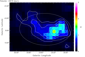
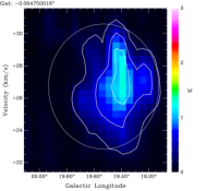
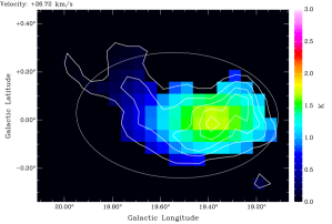
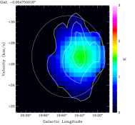
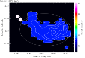
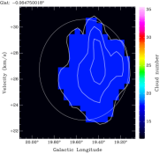
Figure 2: An example of the identification of an isolated molecular cloud in ($\ell$, $b$) and ($\ell$, $v$) space. The left panels show single velocity channel in the ($\ell$, $b$) image, while the right panels show a single Galactic latitude plane in the ($\ell$, $v$) image. The top panels show the smoothed GRS data in color scale. On all images the contours are the smoothed data, while the white ellipses mark the approximate extent of the cloud as determined by CLUMPFIND; the major and minor axes are equivalent to the projected extent of the cloud in each direction. The middle panels show the corresponding Gaussian model, which was generated using the peak temperature, center position, size, orientation, line width, and voxels output from CLUMPFIND. The lower panels show the CLUMPFIND output cube; the color scale in these images represent the voxels that are assigned to each cloud for each particular channel or plane.

Figure 2 shows an example of the identification of an isolated molecular cloud in ($\ell$, $b$) and ($\ell$, $v$) space. Because of the difficulties of displaying three-dimension data cubes in a two-dimensional image, we have selected to show a single velocity channel in the ($\ell$, $b$) image (left panels) and a single Galactic latitude plane in the ($\ell$, $v$) image (right panels). The top panels show an isolated molecular cloud in the smoothed GRS data (in color scale and as contours in this and all subsequent images). The white ellipses mark the approximate extent of the cloud as determined by CLUMPFIND; the major and minor axes are equivalent to the projected extent of the cloud in each direction. The middle panels of Figure 2 show the corresponding Gaussian model, which was generated using the peak temperature, center position, size, orientation, and line width output from CLUMPFIND. The lower panels show the CLUMPFIND output cube; the color scale in these images represent the voxels that are assigned to each cloud for each particular channel or plane.

Williams et al. (1994) found that CLUMPFIND most accurately represents the data when the contour increment is set to twice the 1 $\sigma$ noise of the data. Because we are interested in selecting the largest and brightest molecular clouds in our dataset, we use a contour increment of twice the 10$\sigma$ noise (rather than 1$\sigma$). Thus, to identify clouds we use a contour increment of twice the 10$\sigma$ noise in the smoothed data (0.20 K) and a lowest brightness level of 20$\sigma$ (0.20 K). Our comparisons of the Gaussian models with the original data indicated that these parameters did not produce extremes in either the number of detected clouds or mean residuals. Thus, we consider them suitable for isolating and identifying molecular clouds.

The output from CLUMPFIND was also checked by eye against the original dataset to verify that these parameters could simultaneously identify and separate both bright and compact molecular clouds in addition to diffuse and extended molecular clouds. This choice of input parameters was confirmed to be satisfactory and were adopted to produce the final catalog. Thus, using a contour increment of 0.20 K and a lowest brightness level of 0.20 K CLUMPFIND, identified 848 molecular clouds in the GRS dataset.

For clouds to be selected as real features, CLUMPFIND requires each cloud to have a minimum number of voxels (we set this number to 16). To be confident we are identifying real molecular clouds, we imposed additional size criteria on each cloud before inclusion in the final list. We exclude all clouds that have their measured sizes in any axis less than or equal to the resolution of the smoothed data in that axis (i.e., $\Delta\ell$ or $\Delta b$ $\leq$ 6′  or $\Delta$ V $\leq$ 0.6 km s^-1). We find 18 clouds that meet these criteria. Thus, when we exclude these, the final catalog contains 829 molecular clouds. In the sections below we characterize the properties of these clouds.

3.1.4 Determining sizes of the clouds

Because molecular clouds have complicated morphologies, it is difficult to quantify their shapes and measure their sizes. Although CLUMPFIND determines the extent of each cloud in Galactic longitude and latitude, this determination fails to account for the cloud’s orientation. To more accurately describe their shapes, we modeled the two-dimensional integrated emission for each cloud using a two-dimensional ellipse fitting routine. Two-dimensional integrated intensity maps of each cloud were produced by summing in velocity over all the voxels identified by CLUMPFIND for a given cloud. The center position of the cloud was then determined from the centroid of this velocity integrated image (with all pixels weighted equally regardless of their integrated intensity). The semimajor and semiminor axes were determined by fitting an ellipse to this integrated intensity image. The listed position angle was measured counter-clockwise from the positive Galactic longitude axis. With this convention, a cloud whose major axis lines along the Galactic plane will have a position angle of 0^∘  while one lying perpendicular to the Galactic plane will have a position angle of 90^∘. This method provides a simple description of the cloud’s position, size, and orientation with respect to the Galactic plane.

We have also calculated the projected two-dimensional area for each cloud which was determined by multiplying the total number of pixels within the integrated intensity image by the area of a pixel in square degrees.

3.2 Clumps

Because molecular clouds show structure on all size scales, they typically contain several compact, dense clumps. These clumps presumably represent the compact, dense regions within the molecular clouds where star and cluster formation may take place. To identify these star-forming clumps, we searched for three-dimensional substructure within each of the 829 molecular clouds in ($\ell$, $b$, $v$) space. To achieve this we used the full angular and spectral resolution GRS data and the original CLUMPFIND algorithm.

For each molecular cloud, we search for clumps using only the voxels for that cloud identified by CLUMPFIND as described in the previous section. We also restricted the size of each clump to at least 50 voxels (in total in ($\ell$, $b$, $v$) space) in order to prevent false detections.

The same technique using three-dimensional Gaussian models (as described in $\S$3.1.3) was used to determine the best CLUMPFIND input parameters to identify and separate the clumps within each of the clouds. We selected 10 molecular clouds to test the CLUMPFIND input parameters for clump identification. These molecular clouds were selected to include a range in sizes, emission levels, and substructures. To test the clump identification, we varied the contour increment using values of 0.2, 0.26, 0.36, 0.39 K and the lowest brightness level from 0.52 K to 1.3 K in steps of 1.3 K and examined, by eye, the output from all combinations of these parameters.

We found a contour increment of 0.26 K (2$\sigma$) and a minimum brightness level of 1.30 K (10$\sigma$) was best at isolating and identifying the individual clumps within the clouds. Using these parameters, we identify, in total, 6135 clumps within these clouds. Again, for the final catalog, we exclude all clumps that have sizes smaller than the resolution in any axis (i.e. $\Delta\ell$ or $\Delta b$ $\leq$ 0$\fdg$01 or $\Delta$ V $\leq$ 0.2 km s^-1). Thus, the final clump catalog contains 6124 entries.

3.3 Examples of clouds and clumps

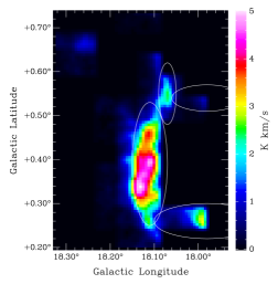
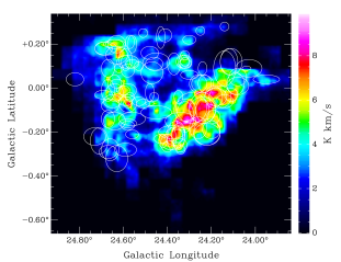
Figure 3: GRSMC G018.14+00.39 (left) and GRSMC G043.34$-$00.36 (right) integrated intensity images. Because it is very difficult to represent the asymmetric, three-dimensional output of CLUMPFIND in a two-dimensional image, we have include on these images white ellipses that indicate the approximate extent of each clump, with the major and minor axes equivalent to the projected extent of the clump in each direction. The identification of clumps is straightforward for GRSMC G018.14+00.39, but more complicated for GRSMC G043.34$-$00.36.

Figure 3 shows the integrated intensity images for two clouds identified in the GRS. The ($\ell,b$)  images were produced by integrating the emission over their velocity range, such that the integrated intensity I = $\int$ T_mb  $dv$. Because it is very difficult to represent the asymmetric, three-dimensional output of CLUMPFIND in a two-dimensional image, we have included on these images white ellipses that indicate the approximate area of the region identified by CLUMPFIND for each clump. To indicate the extent of the clouds, we use two-dimensional ellipses whose major and minor axes are equal to the projected extent of the clump in each direction. The identification clumps is straightforward for GRSMC G018.14+00.39, but more complicated for GRSMC G043.34$-$00.36 (see Fig. 3).

We find the number of clumps within these 829 molecular clouds range from 1 to 111, with a typical molecular cloud containing $\sim$ 7 clumps. Because some clouds are too faint, we detect no clumps within them above the clumpfind threshold. However, most of the clouds ($\sim$ 96%) contain at least one clump that has a peak T_mb  $>$ 10 times the average temperature of the cloud. These are the brightest clumps in the clouds where star-formation will likely occur.

4 Description of the catalog

Table Molecular clouds and clumps in the Boston University–Five College Radio Astronomy Observatory Galactic Ring Survey gives a sample of the catalog entries for each molecular cloud. Table Molecular clouds and clumps in the Boston University–Five College Radio Astronomy Observatory Galactic Ring Survey gives a sample of the catalog entries for the clumps. The complete catalogs are available in electronic format at http://www.bu.edu/galacticring/molecular_clouds.html.

4.1 Clouds

For each molecular cloud identified, we list parameters output from the CLUMPFIND algorithm in addition to several derived quantities. The columns of Table Molecular clouds and clumps in the Boston University–Five College Radio Astronomy Observatory Galactic Ring Survey are as follows: (1) the molecular cloud name, designated as GRSMC (for GRS Molecular Cloud) followed by the Galactic longitude and latitude ($\ell$ and $b$) coordinates of the peak of the emission in degrees, e.g. GRSMC G053.59+00.04; (2), (3) and (4) the Galactic coordinates ($\ell$ and $b$) and velocity (V_LSR) of the peak voxel of the emission; (5) the velocity FWHM defined as 2.35 times the velocity dispersion ($\Delta$ V); (6) main beam temperature of the peak voxel (T_mb); (7) and (8) the Galactic coordinates ($\ell$ and $b$) of the centroid of the integrated intensity image; (9) and (10) the semimajor and semiminor axes (a and b), determined from the elliptical Gaussian fit to the integrated intensity image; (11) position angle of the fitted ellipse, measured counter-clockwise from the positive longitude axis (PA); (12) the projected two-dimensional area (A); (13) the average main beam temperature of the cloud, defined as the average main beam temperature of all the voxels (T_av); (14) the peak integrated intensity (I_peak); (15) the total ¹³CO  integrated intensity (I_total); (16) the peak H₂  column density N(H₂); and (17) a flag denoting if the cloud lies on one of the survey boundaries (’X’, ’Y’ or ’V’ indicate that the cloud lies on the boundary in Galactic longitude, Galactic latitude or velocity, respectively.)

Because molecular clouds have irregular shapes and complex morphologies, the parameters listed in columns (7)–(11) are given simply to estimate the clouds’ approximate position, size, and orientation.

4.2 Clumps

The clumps listed here represent the compact, dense substructures within the clouds. Because we are interested in selecting the brightest, densest regions within each of the clouds, not all clouds have entries in this list; for the faintest clouds, we often detected no clumps. To describe the shape of the clumps we simply use the extent in Galactic longitude and latitude output directly from CLUMPFIND (rather than the elliptical fitting that was performed for the clouds).

The columns of Table Molecular clouds and clumps in the Boston University–Five College Radio Astronomy Observatory Galactic Ring Survey are as follows: (1) the molecular cloud name (from Table Molecular clouds and clumps in the Boston University–Five College Radio Astronomy Observatory Galactic Ring Survey); (2) the clump number, e.g. c1, c2, c3, etc; (3), (4) and (5) the Galactic coordinates ($\ell$ and $b$) and velocity (V_LSR) of the peak voxel of the emission; (6), (7) and (8) the FWHM extent in longitude, latitude and velocity ($\Delta\ell$, $\Delta b$, and $\Delta$ V); (9) the main beam temperature of the peak voxel (T_mb); (10) the projected two-dimensional area (A); (11) the peak integrated intensity (I_peak); (12) the total ¹³CO  integrated intensity (I_total); (13) the peak H₂  column density (N(H₂)); and (14) a flag denoting if the clump lies on a boundary.

5 Ensemble properties

5.1 Galactic distribution

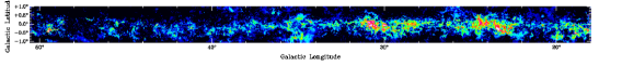
Figure 4: The Galactic distribution of the 829 molecular clouds identified in the GRS. The top panel shows the integrated intensity image for the GRS (square root color scale, from 0 to 40 K km s^-1). The lower panels show the number distribution of molecular clouds in Galactic latitude (left) and longitude (right).

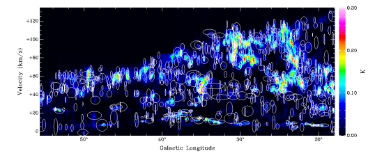
Figure 5: The ($\ell,v$)  diagram for the GRS. The color scale represents the ¹³CO  emission averaged over Galactic latitude. The ellipses mark the approximate extent in Galactic longitude and velocity for each of the 829 clouds identified.

Figure 4 shows the number distribution in Galactic latitude (left) and longitude (right) of the 829 molecular clouds identified in the GRS. Included in this figure for comparison is the integrated intensity image for the GRS, that is the ¹³CO  emission integrated over all velocities. The location of the clouds in ($\ell,v$)  space is shown in Figure 5, overlaid on the GRS ($\ell,v$)  image, which is the ¹³CO  emission averaged over all Galactic latitudes. The clouds identified span the complete range in Galactic longitude, latitude, and velocity as covered by the GRS.

Because the Milky Way rotation is well approximated by an axisymmetric rotation curve, the line of sight velocity directly relates to a Galactocentric radius. Thus, the ($\ell,v$)  positions can uniquely determine Galatocentric radii. To determine Galactocentric radii, we assume circular motions and the rotation curve of Clemens (1985) with (R₀,$\Theta_{0}$) = (8.5 kpc, 220 km s^-1). Because we are sampling clouds primarily in the flat part of the rotation curve, the derived kinematic distances are insensitive to the exact choice of rotation curve. Figure 6 shows the number distribution of clouds as a function of Galactocentric radii. The peaks in this distribution correspond to the known spiral features within the Galaxy.

In the inner Galaxy, a single Galactocentric radius corresponds to two kinematic distances, one at the near distance and one at the far distance. Accurate distances cannot be determined until this ambiguity is resolved. A comparison of GRS data with $\mathrm{H\,{\scriptstyle{I}}}$  self-absorption can resolve this ambiguity and will be presented in a future paper (J. Duval et al. in prep.)

5.2 Properties of the clouds and clumps

Figure 7 shows the number distributions of the clouds (diagonally hashed histograms) and clumps (horizontally hashed histograms) as a function of peak T_mb, line width, semimajor axis, semiminor axis, position angle, and peak H₂  column density.

We find that the clouds have a mean peak ¹³CO  T_mb  of $\sim$ 1.6 K, $\Delta$V of $\sim$ 3.6 km s^-1, semimajor axes of $\sim$ 0$\fdg$41, and semiminor axes of $\sim$ 0$\fdg$23. The fact that the semimajor axes are typically twice the semiminor axes suggests that most clouds are elongated. In fact, the mean value of the ratio of semimajor to semiminor axis is 2.0. On the other hand, we find that the clumps are typically brighter (peak T_mb  of $\sim$ 5.2 K), have lower line widths ($\Delta$V $\sim$ 1.4 km s^-1), are smaller (semimajor axes of 0$\fdg$06), and are rounder (the semimajor and semiminor axes are comparable).

The position angles measured for the clouds range from $-$90 to 90^∘  with a peak value of 1$\fdg$2 (Fig. 7). The position angles were measured counter-clockwise from the positive Galactic longitude axis, so a peak value in the distribution of 1$\fdg$2 implies most clouds are orientated along the Galactic plane. This result is in agreement with previous studies using the GRS dataset (Koda et al., 2006). This result may arise from an observational bias due to the extended areal coverage of the GRS along the Galactic plane ($\sim$ 38^∘  were covered in Galactic longitude compared to the 2^∘  covered in Galactic latitude). The fact that few clouds were detected toward the edges of the coverage in Galactic latitude, however, suggests that our results are not severely effected by this lack of latitude coverage.

The peak H₂  column density, N(H₂), was calculated by assuming optically thin ¹³CO  emission with an excitation temperature of 10K and using standard conversion factors (see Simon et al., 2001) via the expression

$$N(H_{2})=4.92\times 10^{20}\,\,I_{peak}\hskip 22.76228pt(cm^{-2})$$

.

where $I_{peak}$ is the peak integrated intensity (K km s^-1). We find that the clouds have a mean peak N(H₂) of $\sim$ 6.3 $\times$ 10²¹ ${\rm cm}^{-2}$  while the clumps have slightly lower peak column densities of $\sim$ 2.4 $\times$ 10²¹ ${\rm cm}^{-2}$. This is opposite to what is expected if the clumps are the densest parts of clouds where star-formation will likely take place. However, this results is easily explained by the fact that the clump distribution includes all clumps within a cloud, makes the mean of the N(H₂) distribution lower for the clumps compared to the clouds.

Table 4 summarizes these parameters for the clouds and clumps and lists the minimum, maximum, mean, median, standard deviation, and slope of a power-law fit to the distributions. We find that the clouds identified have smaller average brightness temperatures, larger line widths and sizes, and higher peak column densities compared to the clumps.

5.3 Determining the excitation temperatures and opacities

To derive the excitation temperatures (T_ex) and opacities ($\tau$) of the clouds within our catalog, we make use of the ¹²CO $J=1\rightarrow 0$  University of Massachusetts-Stony Brook survey (UMSB; Sanders et al., 1986). The survey region covered the same region of the Galactic plane as the GRS, but mapped the molecular clouds via their ¹²CO  emission. Direct comparisons between the measured ¹²CO  and ¹³CO  temperatures are facilitated by the fact that the two surveys were obtained with the same telescope (the FCRAO 14 m). However, because the UMSB survey was under-sampled (45″  beam on a 3′  grid; Sanders et al., 1986) compared to the GRS (46″  beam on a 22″  grid; Jackson et al., 2006), the combination of the two dataset can only provide rough average values for the entire cloud.

Because the ¹²CO $J=1\rightarrow 0$  emission is typically optically thick, it can be used to estimate the kinetic temperature of the gas via the expression

$$T_{\rm k}=5.532\left[ln\left(1+\frac{5.532}{T_{12}+0.837}\right)\right]^{-1}\hskip 22.76228pt(K)$$

where T₁₂ is the ¹²CO  brightness temperature measured from the UMSB survey. The kinetic temperature can then be used to calculate the opacities for the optically thin ¹³CO $J=1\rightarrow 0$  transition using

$$\tau\approx\frac{kT_{mb}}{h\nu}\left[\frac{1}{e^{\frac{h\nu}{kT_{k}}}-1}-\frac{1}{e^{\frac{h\nu}{kT_{bg}}}-1}\right]^{-1}$$

where T_bg is 2.7 K and T_mb  is the ¹³CO  brightness temperature measured within the cloud from the GRS. To calculate T₁₂ and T₁₃ we calculate the mean T_mb  from all the corresponding voxels associated with each cloud as defined by CLUMPFIND within the UMSB and GRS datasets respectively. The excitation temperature of the gas is then calculated using

$$T_{ex}=\frac{T_{mb}}{(1-e^{-\tau})}+T_{bg}\hskip 22.76228pt(K)$$

Figure 8 shows the histograms of T_ex  and $\tau$ for the clouds. We find that the clouds typically have T_ex  of $\sim$ 9 K and a ¹³CO  $\tau$ of 0.13 (see Table 4 for a summary). Most clouds have low opacities, which confirms the fact that the ¹³CO  is optically thin and, thus, a good tracer of the column density and mass.

5.4 Properties of clouds inside and outside the 5 kpc ring

With a large sample of molecular clouds we can now investigate their properties in a range of Galactic environments. For instance, does the temperature, line width, and column density of the molecular clouds within active star-forming regions differ from those in more quiescent regions? Given that the majority of Galactic star formation occurs within the 5 kpc molecular ring, one might expect to see differences in the properties of the molecular clouds within the ring, compared to clouds that lie outside the ring.

To test this idea we have separated the clouds identified with the GRS into those that lie inside the 5 kpc molecular ring from those that lie outside the ring. We have defined clouds that are associated with the peak in the Galactocentric radius (R_G) distribution (Fig. 6) at $\sim$ 4.5 kpc as those associated with the ring (i.e. all clouds with 4 kpc $<$ R_G $<$ 5 kpc). Thus, the number of clouds within the ring, N_in, is 206 (25%), while the number of clouds outside the ring, N_out, is 623 (75%).

Figure 9 shows the number of clouds in and out of the ring (solid and open histograms respectively) plotted against their values of T_ex, $\tau$, line width, peak N(H₂), area, and number of clumps. Included in the top panels of each of these plots is the fraction of clouds within the ring in each of the bins. These plots show that clouds within the ring typically have warmer temperatures, higher column densities, larger areas, and more clumps compared to clouds located outside the ring. The mean opacities appear comparable between clouds inside and outside the ring. We also find clouds within the ring have similar mean values of the line width compared to those clouds outside the ring.

In addition to the general cloud properties, we have also performed a K-S test for each of the properties to determine if the distribution in the samples inside and outside of the 5 kpc ring are derived from the same parent distribution. Table 4 lists the results of the K-S tests and shows that for all properties, with the exception of position angles, the distributions are not derived from the same parent distribution. Thus, there are clear, and significant differences in the distributions of the derived properties for the clouds inside and outside the 5 kpc molecular ring.

Warmer temperatures and higher column densities are exactly what is expected for active star-forming regions. All the clouds have line widths much greater than the thermal line width for gas at their derived T_k  (for T_k= 10 K, the thermal line width for CO is 0.13 km s^-1) suggesting that they are dominated by turbulent motions.

The fact that we see more clumps within the clouds associated with the 5 kpc molecular ring also strengthens the idea that these clouds are forming stars. This suggests that clouds within the ring are highly fragmented and have many dense, warm regions where the star formation can occur, in contrast to the more quiescent, smoother clouds outside the ring.

While these results suggest that clouds within the ring have different properties to those clouds found outside the ring, we need to consider that clouds within the ring suffer more from line blending and their identification as separate features or merged clouds is more dependent on the values input into CLUMPFIND. Moreover, the effects of distance also need to be considered; we can more easily separate nearby clouds as opposed to those at the far side of the Galaxy. Nevertheless, our analysis suggests that the clouds within the ring are significantly different from those outside the ring.

6 Summary

Using the CLUMPFIND algorithm we have identified a large sample of clouds and clumps within the ¹³CO $J=1\rightarrow 0$ BU–FCRAO Galactic Ring Survey. In total, we identified 829 clouds and 6124 clumps. We find the cloud properties are comparable to typical Giant Molecular Clouds, while the clumps are similar to the regions where star and cluster formation occur. Moreover, it appears that clouds lying within the 5 kpc ring typically have warmer temperatures, higher column densities, larger areas, higher densities, higher masses, and more clumps compared to clouds located external to the ring. This difference supports the idea that star formation occurs within the ring. We note, however, that there are inherent difficulties in determining cloud properties without the proper consideration of distance biases.

This catalog provides an invaluable tool for studies of molecular clouds. For instance, establishing reliable kinematic distances to the GRS molecular clouds and clumps, and to their embedded young stellar objects and clusters, is essential in order to determine their masses, sizes, distributions, and luminosities. Thus, combining the catalog of GRS molecular clouds with IR Galactic plane surveys from IRAS, MSX, 2MASS, and Spitzer, one can obtain luminosities, masses, and sizes of stars and clusters embedded within their natal molecular material. One can then address the questions: What is is the spatial distribution, luminosity function, and initial mass function of the young stars forming both inside and outside the ring? How does the star-formation process within the ring differ from that at other locations in the Galaxy, such as near the Sun, in nearby spiral arms, and in the outer Galaxy? Moreover, the internal structure of molecular clouds, which traces the influence of turbulence in the interstellar medium, can also be studied in a wide range of star-forming environments. With a large sample of clouds we can also obtain their clump mass spectra and study its relation to the stellar initial mass function. These are all important and outstanding questions relating to Galactic star-formation.

Figure 6: Galactocentric radial distribution of the molecular clouds identified in the GRS.

Figure 7: Normalized number distributions for the measured parameters T_mb, line width, semimajor and semiminor axis, position angle, and peak N(H₂) for the clouds (diagonally hashed histogram) and clumps (horizontally hashed histogram). Position angles were only calculated for the clouds. See Table 4 for a summary of these distributions.

Figure 8: Number distributions of the excitation temperature, T_ex, (left) and the ¹³CO  opacities, $\tau$, (right) for the clouds. These were calculated by combining the ¹³CO  GRS emission with ¹²CO $J=1\rightarrow 0$  emission from the University of Massachusetts-Stony Brook survey (UMSB; Sanders et al., 1986). The molecular clouds have mean T_ex  of $\sim$ 9 K and $\tau$ of 0.13.

Figure 9: Histograms of the parameters for clouds located in the 5 kpc molecular ring (solid histogram) and outside the ring (open histograms). The top panel in each plot shows the fraction of the number of clouds in the ring for each bin. We find that the clouds within the ring typically have warmer temperatures, higher column densities, larger areas, and more clumps compared to clouds located outside the ring. This is expected if these clouds are actively forming stars.

Table 1: Properties of Giant Molecular clouds, clumps, and cores (Goldsmith, 1987; Cernicharo, 1991).

Properties		GMC	Clump	Core
Size (pc)		20–60	3–20	0.5–3
Density (${\rm cm}^{-3}$)		100–300	103–104	104–106
Mass ($M_{\odot}$)		104–106	103–104	10–103
Linewidth (km s-1)		6–15	4–12	1–3
Temperature (K)		7–15	15–40	30–100

Table 2: Properties of the molecular clouds identified in the GRS.

Cloud	Peak		VLSR	$\Delta$V	Tmb	Centroid		a	b	PA	A	Tav	Ipeak	Itotal	N(H2)	Flag
GRSMC	$\ell$	$b$				$\ell$	$b$
	(∘)	(∘)	(km s-1)	(km s-1)	(K)	(∘)	(∘)	(∘)	(∘)	(∘)	(deg2)	(K)	(K km s-1)	(K km s-1 deg2)	($\times$1022 cm-2)
(1)	(2)	(3)	(4)	(5)	(6)	(7)	(8)	(9)	(10)	(11)	(12)	(13)	(14)	(15)	(16)	(17)
G053.59+00.04	53.59	0.04	23.7	1.99	5.75	53.69	0.01	0.52	0.19	16	0.27	1.90	36.5	0.95	1.8	-
G029.89$-$00.06	29.89	$-$0.06	100.7	5.09	5.46	29.99	$-$0.17	0.44	0.35	-46	0.46	2.49	87.6	3.12	4.3	-
G049.49$-$00.41	49.49	$-$0.41	56.9	9.77	5.25	49.57	$-$0.39	0.38	0.23	-21	0.18	2.18	193.2	1.64	9.5	Y
G018.89$-$00.51	18.89	$-$0.51	65.8	2.80	5.17	18.80	$-$0.56	0.31	0.31	-47	0.29	2.31	57.5	1.51	2.8	-
G030.49$-$00.36	30.49	$-$0.36	12.3	4.56	4.98	30.66	$-$0.39	0.47	0.24	-28	0.22	1.70	17.5	0.50	0.9	-
G035.14$-$00.76	35.14	$-$0.76	35.2	5.00	4.92	35.22	$-$0.78	0.31	0.22	-11	0.20	2.36	59.3	1.90	2.9	Y
G034.24+00.14	34.24	0.14	57.8	5.98	4.81	34.19	0.05	0.50	0.41	-3	0.52	1.46	80.5	3.15	4.0	-
G019.94$-$00.81	19.94	$-$0.81	42.9	2.81	4.58	19.97	$-$0.80	0.42	0.18	-7	0.22	1.76	32.1	1.00	1.6	Y
G023.44$-$00.21	23.44	$-$0.21	101.1	5.75	4.40	23.36	0.02	0.64	0.48	29	0.63	1.65	63.2	3.71	3.1	-
G038.94$-$00.46	38.94	$-$0.46	41.6	2.97	4.33	39.01	$-$0.51	0.36	0.28	-10	0.23	1.90	31.8	1.02	1.6	-
G023.44$-$00.21	23.44	$-$0.21	103.7	3.44	4.23	23.55	$-$0.27	0.35	0.23	28	0.12	2.13	51.7	0.49	2.5	-
G030.79$-$00.06	30.79	$-$0.06	94.7	6.12	4.23	30.86	$-$0.04	0.39	0.28	66	0.32	2.24	79.5	2.68	3.9	-
G030.29$-$00.21	30.29	$-$0.21	104.5	3.01	3.92	30.36	$-$0.18	0.39	0.23	66	0.26	1.66	40.0	0.98	2.0	-
G053.14+00.04	53.14	0.04	22.0	2.39	3.88	53.15	0.09	0.42	0.26	74	0.29	2.01	26.8	0.93	1.3	-
G022.44+00.34	22.44	0.34	84.5	2.81	3.62	22.51	0.30	0.41	0.23	32	0.14	1.52	29.0	0.42	1.4	-
G024.49+00.49	24.49	0.49	102.4	5.24	3.58	24.48	0.30	0.52	0.32	8	0.46	1.46	67.8	2.21	3.3	-
G049.39$-$00.26	49.39	$-$0.26	50.9	3.54	3.54	49.44	$-$0.23	0.30	0.18	63	0.15	1.93	54.1	0.90	2.7	-
G019.39$-$00.01	19.39	$-$0.01	26.7	3.88	3.48	19.53	0.02	0.42	0.26	-2	0.31	1.73	39.0	2.00	1.9	-
G034.74$-$00.66	34.74	$-$0.66	46.7	4.33	3.46	34.88	$-$0.63	0.42	0.34	51	0.34	1.91	35.3	2.27	1.7	Y
G023.04$-$00.41	23.04	$-$0.41	74.3	4.20	3.40	23.07	$-$0.45	0.50	0.31	7	0.45	1.54	45.9	2.31	2.3	-
G018.69$-$00.06	18.69	$-$0.06	45.4	3.86	3.33	18.77	$-$0.13	0.26	0.18	-22	0.13	1.87	32.8	0.85	1.6	-
G018.19$-$00.31	18.19	$-$0.31	50.1	4.15	3.29	18.20	$-$0.44	0.39	0.27	89	0.27	1.89	52.5	1.52	2.6	X
G025.64$-$00.11	25.64	$-$0.11	93.9	2.78	3.21	25.67	$-$0.26	0.36	0.30	12	0.29	1.64	24.8	1.06	1.2	Y
G024.79+00.09	24.79	0.09	110.4	3.25	3.17	24.62	0.17	0.48	0.37	4	0.48	1.50	50.3	1.79	2.5	-

Table 3: Properties of the molecular clumps identified in the GRS.

Table 4: Summary of the derived properties of the GRS molecular clouds and clumps.

Properties	Clouds								Clumps
	Min	Max	Mean	Median	Std dev	Slope	K-S test		Min	Max	Mean	Median	Std dev	Slope
Peak Tmb  temperature (K)	0.8	5.8	1.6	1.4	0.7	$-$3.1 $\pm$ 0.2	0.000000		1.2	27.3	5.2	4.7	2.0	$-$4.0 $\pm$ 0.3
Linewidth (km s-1)	0.6	9.8	3.6	3.4	1.4	$-$2.9 $\pm$ 0.4	0.001645		0.2	8.3	1.4	1.2	0.8	$-$3.1 $\pm$ 0.4
Semimajor Axis (degs)	0.06	1.16	0.41	0.41	0.15	$-$5.3 $\pm$ 0.3	0.000014		0.01	0.25	0.03	0.02	0.02	$-$2.3 $\pm$ 0.2
Semiminor Axis (degs)	0.05	0.53	0.23	0.22	0.09	$-$2.7 $\pm$ 0.5	0.000138		0.01	0.24	0.03	0.02	0.02	$-$2.0 $\pm$ 0.3
Position Angle (degs)	-90.0	90.0	1.2	-1.0	43.5		0.965160
Log[Peak H2  column density (${\rm cm}^{-2}$)]	20.7	23.0	21.8	21.8	0.3	$-$2.3 $\pm$ 0.2	0.000000		20.8	22.1	21.4	21.4	0.2	$-$4.1 $\pm$ 0.2
Excitation Temperature (K)	4.1	17.5	8.8	8.5	2.0	$-$6.8 $\pm$ 0.6	0.000001
Opacity	0.07	0.50	0.13	0.12	0.04	$-$3.7 $\pm$ 0.3	0.000231
Radius (pc)	1.6	97.5	24.1	22.6	12.5	$-$4.0 $\pm$ 0.4	0.002011		1.2	27.3	5.2	4.7	2.0	$-$4.1 $\pm$ 0.2
Log[LTE Mass ($M_{\odot}$)]	2.2	5.7	4.5	4.6	0.6	$-$1.8 $\pm$ 0.3	0.000000		0.2	5.3	2.9	2.9	0.7	$-$1.2 $\pm$ 0.1
Log[Virial Mass ($M_{\odot}$)]	1.9	5.7	4.5	4.5	0.6	$-$1.5 $\pm$ 0.2	0.000532		0.3	5.2	2.7	2.7	0.7	$-$1.2 $\pm$ 0.1
Log[Density (${\rm cm}^{-3}$)]	0.6	2.8	1.7	1.7	0.4	$-$1.4 $\pm$ 0.2	0.000000		0.8	3.6	2.5	2.6	0.4	$-$2.9 $\pm$ 0.4

References

- Burton (1976) Burton, W. B. 1976, ARA&A, 14, 275
- Cernicharo (1991) Cernicharo, J. 1991, in NATO ASIC Proc. 342: The Physics of Star Formation and Early Stellar Evolution, 287
- Clemens (1985) Clemens, D. P. 1985, ApJ, 295, 422
- Clemens et al. (1988) Clemens, D. P., Sanders, D. B., & Scoville, N. Z. 1988, ApJ, 327, 139
- Combes (1991) Combes, F. 1991, ARA&A, 29, 195
- Dame et al. (2001) Dame, T. M., Hartmann, D., & Thaddeus, P. 2001, ApJ, 547, 792
- Goldsmith (1987) Goldsmith, P. F. 1987, in Astrophysics and Space Science Library, Vol. 134, Interstellar Processes, ed. D. J. Hollenbach & H. A. Thronson, Jr., 51–70
- Jackson et al. (2006) Jackson, J. M., Rathborne, J. M., Shah, R. Y., Simon, R., Bania, T. M., Clemens, D. P., Chambers, E. T., Johnson, A. M., Dormody, M., Lavoie, R., & Heyer, M. H. 2006, ApJS, 163, 145
- Koda et al. (2006) Koda, J., Sawada, T., Hasegawa, T., & Scoville, N. Z. 2006, ApJ, 638, 191
- Robinson et al. (1984) Robinson, B. J., Manchester, R. N., Whiteoak, J. B., Sanders, D. B., Scoville, N. Z., Clemens, D. P., McCutcheon, W. H., & Solomon, P. M. 1984, ApJ, 283, L31
- Sanders et al. (1986) Sanders, D. B., Clemens, D. P., Scoville, N. Z., & Solomon, P. M. 1986, ApJS, 60, 1
- Scoville & Solomon (1975) Scoville, N. Z. & Solomon, P. M. 1975, ApJ, 199, L105
- Simon et al. (2001) Simon, R., Jackson, J. M., Clemens, D. P., Bania, T. M., & Heyer, M. H. 2001, ApJ, 551, 747
- Williams et al. (1994) Williams, J. P., de Geus, E. J., & Blitz, L. 1994, ApJ, 428, 693