Optical determination of the relation between the electron-boson coupling function and the critical temperature in high T_c cuprates.

Abstract

We take advantage of the connection between the free carrier optical conductivity and the glue function in the normal state, to reconstruct from the infrared optical conductivity the glue-spectrum of ten different high-T_c cuprates revealing a robust peak in the 50-60 meV range and a broad continuum at higher energies for all measured charge carrier concentrations and temperatures up to 290 K. We observe that the strong coupling formalism accounts fully for the known strong temperature dependence of the optical spectra of the high T_c cuprates, except for strongly underdoped samples. We observe a correlation between the doping trend of the experimental glue spectra and the critical temperature. The data obtained on the overdoped side of the phase diagram conclusively excludes the electron-phonon coupling as the main source of superconducting pairing.

I Introduction.

The theoretical approaches to the high T_c pairing mechanism in the cuprates are divided in two main groups: According to the first electrons form pairs due to a retarded attractive interaction mediated by virtual bosonic excitations in the solidscalapino-PRB-1986 ; varma-PRL-1989 ; millis-PRB-1990 ; dolgov-physc-1991 ; abanov-spec-2001 . These bosons can be lattice vibrations, fluctuations of spin-polarization, electric polarization or charge density. The second group of theories concentrates on a pairing-mechanism entirely due to the non-retarded Coulomb interactionanderson-sci-2007 or so-called Mottnessphillips-annphys-2006 . Indeed, optical experiments have found indications for mixing of high and low energy degrees of freedom when the sample enters into the superconducting statebasov-sci-1999 ; molegraaf-science-2002 ; carbone-PRB-2006a ; carbone-PRB-2006b .

An indication that both mechanisms are present was obtained by Maier, Poilblanc and Scalapinomaier-PRL-2008 , who showed that the ’anomalous’ self-energy associated with the pairing has a small but finite contribution extending to an energy as high as $U$, demonstrating that the pairing-interaction is, in part, non-retarded. The experimental search for a pairing glue will play an essential role in determining the origin of the pairing interaction. Aforementioned glue is expressed as a spectral density of these bosons, indicated as $\alpha^{2}F(\omega)$ for phonons and $I^{2}\chi(\omega)$ for spin fluctuations, here represented as the general, dimensionless function $\tilde{\Pi}(\omega)$. An important consequence of the electron-boson coupling is, that the energy of the quasi-particles relative to the Fermi level, $\xi$, is renormalized, and their lifetime becomes limited by inelastic decay processes involving the emission of bosons. The corresponding energy shift and the inverse lifetime, i.e. the real and imaginary parts of the self-energy, are expressed as the convolution of the ’glue-function’ $\tilde{\Pi}(\omega)$ with a kernel $K(\xi,\omega,T)$ describing the thermal excitations of the glue and the electronskernel

$$\Sigma(\xi)=\int K(\xi,\omega,T)\tilde{\Pi}(\omega)d\omega$$ (1)

In the absence of a glue and of scattering off impurities the effect of applying an AC electric field to the electron gas is to induce a purely reactive current response, characterized by the imaginary optical conductivity $4\pi\sigma(\omega)=i\omega_{p}^{2}/\omega$, where the plasma frequency, $\omega_{p}$, is given by the (partial) f-sum rule for the conduction electrons. The effect of coupling the electrons to bosonic excitations is revealed by a finite, frequency dependent dissipation, which can be understood as arising from processes whereby a photon is absorbed by the simultaneous creation of an electron-hole pair and a boson. As a result, the expression for the optical conductivity in the normal state,

$$4\pi\sigma(\omega)=\frac{i\omega_{p}^{2}}{\omega+\hat{M}(\omega)},$$ (2)

now contains a memory function or optical self energygotze-PRB-1972 ; timusk-footnote . A particularly useful aspect of this representation is that $\hat{M}(\omega)$ follows in a straightforward way from the experimental optical conductivity. The optical self-energy is related to the single particle self-energies by the expressionpballen-PRB-1971

$$\frac{\hat{M}(\omega)}{\omega}=\left\{{\int\frac{f(\xi)-f(\xi+\omega)}{\omega+\Sigma^{*}(\xi)-\Sigma(\xi+\omega)}d\xi}\right\}^{-1}-1$$ (3)

The central assumption in the above is the validity of the Landau Fermi-liquid picture for the normal state. The aforementioned strong coupling analysis is therefore expected to work best on the overdoped side of the cuprate phase diagram, where the state of matter appears to become increasingly Fermi liquid like. If antiferromagnetism is necessary to obtain the insulating state in the undoped parent compounds, as has been argued based on the doping trends of the Drude spectral weightmillis-nphys-2008 , the strong coupling analysis may in principle be relevant for the entire doping range studied. However, in the limit of strong interactions aforementioned formalism needs to be extended, e.g. with vertex corrections, and it eventually breaks down. We therefore define the function $\tilde{\Pi}(\omega)$ as the effective quantity which, in combination with Eqs. 1 and 3, returns the exact value of $\hat{M}(\omega)$ for each frequency. Defined in this way $\tilde{\Pi}(\omega)$ captures all correlation effects regardless whether the system is a Fermi-liquid or not. This becomes increasingly relevant when the doping is lowered below optimal doping.

Here we take advantage of the connection between the temperature and frequency dependent conductivity in the normal state and the glue-spectrum to test experimentally the consequences of the standard approach, to check the internal consistency of it, and to determine the range of doping where internal consistency is obtained. For a d-wave superconductor, the momentum dependence is essential to understand the details of the pairing. This, of course, is difficult to handle for optical spectroscopy which is inherently a momentum integrated probe. Nevertheless, optical spectra provide the important information on the energy scale of the bosons involved and on the doping and temperature evolution. The paper is organized as follows. In section II we show that the temperature dependence of the optical spectra of the cuprates is well described within the strong coupling formalism described above. In section III we present the $\tilde{\Pi}(\omega)$ functions for 10 different cuprates. These $\tilde{\Pi}(\omega)$ functions are used in section IV to estimate critical temperatures and section V discusses the implications of these results with regard to the pairing mechanism in the cuprates. Finally, in section VI we summarize our results.

II Internal consistency check of the strong coupling formalism.

In order to test whether the strong coupling analysis is applicable to the cuprates we start with an important test of its internal consistency: (i) we invert the data at 290 K to obtain $\tilde{\Pi}(\omega)$, (ii) we use this $\tilde{\Pi}(\omega,290K)$ to predict the optical spectra at lower temperatures. If the prediction faithfully reproduces the experimental spectra at these temperatures, we have a strong indication that the electronic structure and its evolution as a function of temperature are to a good approximation within the realm of strong coupling theory. We use a standard least squares routine to fit a histogram representation of $\tilde{\Pi}(\omega)$ to our experimental infrared spectra (see Appendix). The quantity $\tilde{\Pi}(\omega)$ is shown in Fig. 1 for optimally doped HgBa₂CuO_4+δ (Hg-1201)heumen-PRB-2007 for $T=290$ K, together with the optical self energies calculated from this function at three different temperatures. For 290 K the theoretical curve runs through the data points, reflecting the full convergence of the numerical fitting routine.

It is interesting to notice, that the shoulder at 80 meV in the 100 K experimental data is reproduced by the same $\tilde{\Pi}(\omega)$ function as the one used to fit the 290 K data. It can be excluded that this shoulder is due to the pseudo-gap, since a gap is certainly absent for temperatures as high as 290 K. The shoulder is therefore entirely due to coupling of the electrons to a mode at approximately 60 meV. On the other hand, the considerable sharpening of this feature for temperatures lower than 100 K finds a natural explanation in the opening of a gap, as illustrated in the inset of Fig. 1. We see that for 100 K the theoretical prediction also runs through the experimental data points. In other words, the strong temperature dependence of the experimental optical spectra is entirely due to the Fermi and Bose factors of Eqs. 1 and 3.

This example confirms the close correspondence between the features in $\hat{M}(\omega)$ and in $\tilde{\Pi}(\omega)$ pointed out in Ref. [norman-PRB-2006, ]. In particular the broad maximum in $\hat{M}(\omega)$ has its counterpart in the high intensity region of $\tilde{\Pi}(\omega)$ terminating at 290 meV.

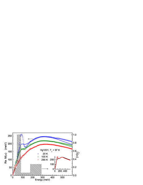
Figure 1: Experimental optical self energy of HgBa₂CuO_4+δ for 3 selected temperatures (open circles). The solid curve at 290 Kelvin is obtained from a fit of $\tilde{\Pi}(\omega)$ , shown as the dashed surface. The solid curves at 100 K and 20 K were calculated with the same $\tilde{\Pi}(\omega)$ function corresponding to 290 Kelvin. This proves that the self energy feature between 80 and 100 meV (a shoulder at 100 K and a peak at 20 K) is caused by the prominent peak in $\tilde{\Pi}(\omega)$ at approximately 60 meV. The sharpening of this feature at low temperature is due to the superconducting gap, an aspect not captured by Eq. 3 and therefore not reproduced in the calculated solid curves. In the inset the gap-induced sharpening is illustrated by the optical self energy without (black) and with (red) a 15 meV superconducting gap, calculated using Allen’s relationpballen-PRB-1971 .

The internal consistency is therefore demonstrated by the fact that the large temperature dependence of the optical spectra is fully explained by the strong coupling formalism. This consistency was obtained for all samples, except for the most strongly underdoped single layer Bi2201 sample.

III Electron boson coupling function.

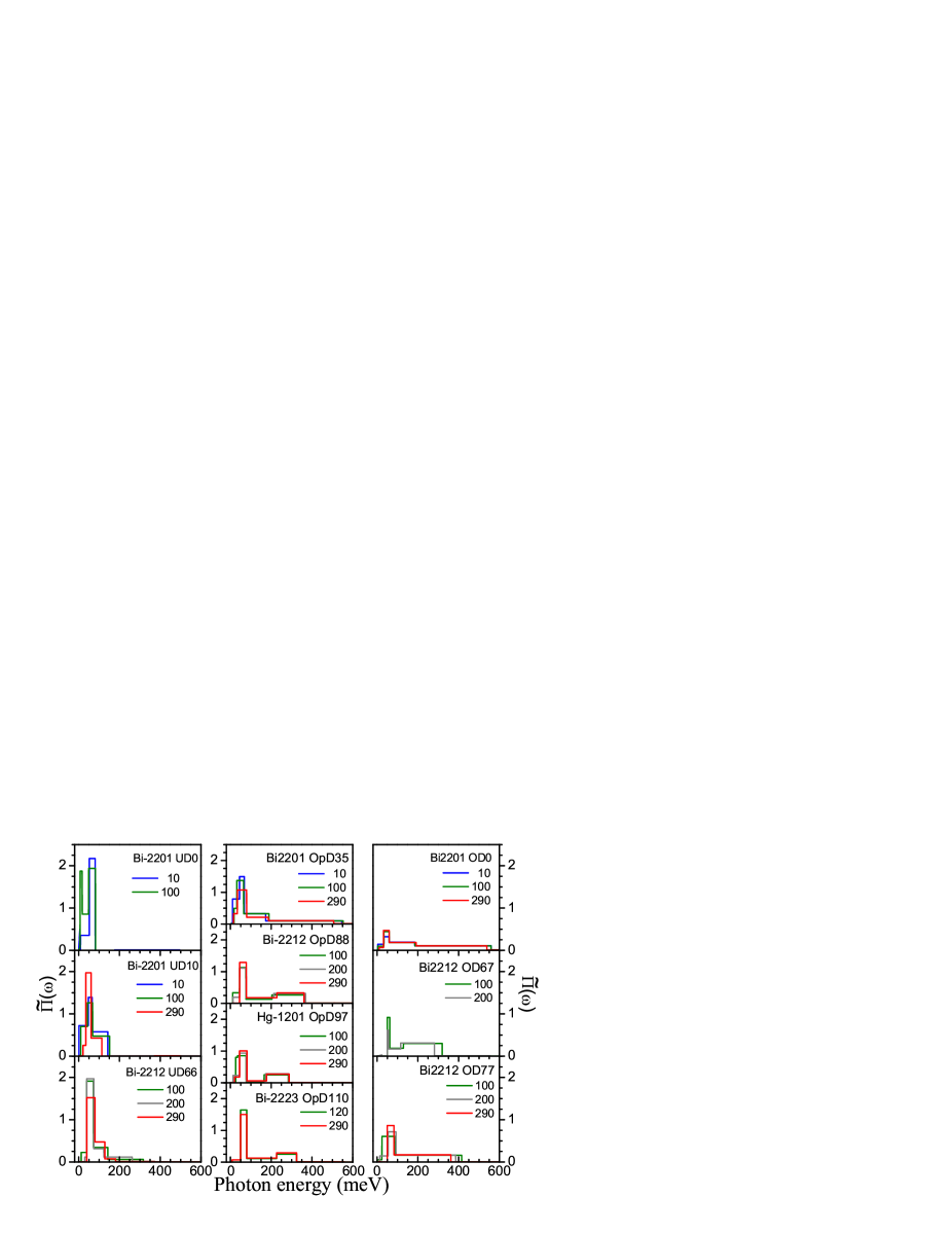
Figure 2: Electron-boson coupling function $\tilde{\Pi}(\omega)$ for Bi-2201 at four different charge carrier concentrations (10 K, 100 K, 290 K), Bi-2212 at four charge carrier concentrations, and optimally doped Bi-2223 and Hg-1201 (100 K, 200 K, 290 K). The samples are ordered from underdoped to overdoped (left to right) and low to high T_c (top to bottom)

As summarized in Fig. 2, we have analyzed previously published optical spectra of 10 different samples belonging to different families of materials, i.e. optimally doped Hg-1201heumen-PRB-2007 and Bi₂Sr₂Ca₂Cu₃O_10+δ (Bi-2223)carbone-PRB-2006b , as well as four Bi₂Sr₂CaCu₂O_8+δ (Bi-2212) crystals molegraaf-science-2002 ; carbone-PRB-2006a with different hole concentrations. In addition, we analyzed data for four Bi₂Sr₂Cu₂O_6+δ (Bi-2201) crystals with different hole concentrationsheumen-NJP-2009 .

Excellent fits were obtained for all temperatures, but the $\tilde{\Pi}(\omega)$ spectra exhibit a significant temperature dependence, in particular at the low frequency side of the $\tilde{\Pi}(\omega)$ spectrum. Since all thermal factors contained in Eqs. 1 and 3 are, in principle, folded out by our procedure, the remaining temperature dependence of $\tilde{\Pi}(\omega)$ reflects the thermal properties of the ’glue-function’ itself. Such temperature dependence is a direct consequence of the peculiar DC and far infrared conductivity, in particular the $T$-linear DC resistivity and $\omega/T$ scaling of $T\sigma(\omega,T)$ at optimal dopingdirk-nature-2003 . For the highest doping levels both $\tilde{\Pi}(\omega)$ and its temperature dependence diminish, which is an indication that a Fermi liquid regime is approached. The most strongly underdoped sample, Bi-2201-UD0, exhibits an upturn of the imaginary part of the experimental optical self-energy for $\omega\rightarrow 0$. This aspect of the data can not be reproduced by the strong coupling expression, resulting in an artificial and unphysical peak at $\omega\approx 0$ of the fitted $\tilde{\Pi}(\omega)$ function.

We observe two main features in the glue-function: A robust peak at 50-60 meV and a broad continuum. The upper limit of $\tilde{\Pi}(\omega)$ is situated around approximately 300 meV for optimally doped single layer Hg1201, and for the bilayer and trilayer samples. The continuum extends to the highest energies (550 meV for the single-layer samples and 400 meV for the bilayer) for the weakly overdoped samples, whereas the continuum of the strongly doped bilayer sample extends to only 300 meV. There is also a clear trend of a contraction of the continuum to lower energies when the carrier concentration is reduced. Hence, part of the glue function has an energy well above the upper limit of the phonon frequencies in the cuprates ($\sim$ 100 meV). Consequently the high energy part of $\tilde{\Pi}(\omega)$ reflects in one way or another the strong coupling between the electrons themselves.

The most prominent feature, present in all spectra reproduced in Fig. 2, is a peak corresponding to an average frequency of 60 $\pm$ 3 meV at room temperature (see Appendix for an estimate of the error bar). Perhaps the most striking aspect of this peak is the fact that its energy is practically independent of temperature (up to room temperature) and sample composition. Moreover, the intensity and width are essentially temperature independent. While our results confirm by and large the observations of Hwang et al. in the pseudo-gap phasetimusk4 ; timusk5 , the persistence of the 50-60 meV peak to room temperature has not been reported before for these compounds. However, Collins et al obtained excellent fits to their infrared data of YBa₂Cu₃O₇ at 100 K and 250K using for both temperatures the same $\alpha^{2}F(\omega)$ spectrum with a peak at $\sim 35$ meV and a continuum extending up to 300 meV. The 50-60 meV peak which we observe, arises most likely from the same boson that is responsible for the ’kink’ seen in angle resolved photoemission (ARPES) experiments along the nodal direction in k-space at approximately the same energybogdanov-PRL-2000 ; lanzara-NAT-2001 ; non-PRL-2006 . The peak-dip-hump structure in the tunneling spectra (STS)lee-nat-2006 ; levy-condmat-2007 ; zasad-PRL-2001 has also been reported at approximately the same energy.

IV Critical temperatures

x		0.09	0.11	0.16	0.22	0.11	0.16	0.20	0.21	0.16	0.16
$T_{c}$	K	0	10	35	0	66	88	77	67	110	97
$\hbar\omega_{p}$	eV	1.75	1.77	1.92	1.93	2.36	2.35	2.45	2.33	2.43	2.10
$\hbar\tilde{\omega}$	meV	-	70	81	103	92	124	116	154	101	81
$\lambda$		-	2.96	2.95	1.42	2.66	2.15	1.50	0.97	2.18	1.85
$\lambda_{pk}$		-	2.85	2.47	0.95	2.36	1.53	1.07	0.35	1.75	1.5
$\lambda_{cnt}$		-	0.11	0.48	0.47	0.3	0.62	0.44	0.62	0.43	0.35
$T_{c,pk}$	K	-	160	140	64	169	123	90	22	132	110
$T_{c,cnt}$	K	-	5	116	113	26	184	101	154	101	64

Table 1: Strong coupling parameters of the ten compounds. The hole-doping is indicated on the first line. From left to right: Bi2201 (columns 1 to 4), Bi2212 (columns 5 to 8), Bi2223 (9th column) and Hg1201 (column 10). On rows 6-9 we indicate the partial coupling constants $T_{c}$’s obtained when the $\tilde{\Pi}(\omega)$ spectra are separated in a contribution from the peak (pk, $\omega\leq$ 100 meV) and from the continuum (cnt, $\omega\geq$ 100) meV. All values are listed for room temperature.

One of the most important issues in the field of high T_c is the question whether pairing is caused by the exchange of virtual bosons. These processes are described by a bosonic density of states function closely related to $\tilde{\Pi}(\omega)$ . If the electron-electron interaction occurs uniquely in the $d$-wave channel, the superconducting critical temperature follows from the usual relation

$$T_{c}=0.83\tilde{\omega}\exp(-(1+\lambda_{d})/\lambda_{d}),$$ (4)

where $\lambda_{d}$ is the coupling constant in the $d$-wave pairing channel is

$$\lambda_{d}=2\int_{0}^{\infty}\tilde{\Pi}_{d}(\omega)/\omega d\omega,$$ (5)

and $\tilde{\Pi}_{d}(\omega)$ is the d-wave electron-boson coupling function. The effective frequency of the bosons responsible for the pairing interaction is obtained by taking the average of $\ln(\omega)$ weighted by electron-boson coupling functioncarbotte ,

$$\ln(\tilde{\omega})=2\lambda^{-1}\int_{0}^{\infty}\omega^{-1}\tilde{\Pi}_{d}(\omega)\ln(\omega)d\omega.$$ (6)

To apply Eq. 4 to our experimentally measured $\tilde{\Pi}(\omega)$ , we would need to map this function on the $d$-wave pairing channel. Boson fluctuations below a certain critical frequency act as pair breakers, as has been shown by Millis, Varma and Sachdevmillis-PRB-1988 in the case of spin-fluctuation-mediated d-wave superconductivity. Clearly, it is not possible to separate pair-breaking from pair-forming contributions to $\tilde{\Pi}(\omega)$ in an unambiguous way. To proceed we assume that the full $\tilde{\Pi}(\omega)$ function contributes favorably to the pairing. This means that our results overestimate the critical temperature. In Table 1 we indicate the total coupling constant, $\lambda$, and logarithmic frequency, $\tilde{\omega}$, for the room temperature $\tilde{\Pi}(\omega)$ spectra. The coupling strength shows a strong and systematic increase with decreasing hole concentration, which probably requires a theoretical treatment beyond the strong coupling expansion. At the same time we see that $\tilde{\omega}$ shows the opposite trend.

An estimate of $T_{c}$, using the experimental values indicated in Table 1, gives values in the 100-200 K range. The critical temperature can also be calculated straightforwardly from the s-wave Eliashberg equationsowen-phys-1971 when $\tilde{\Pi}(\omega)$ is known. As shown in Fig. 3, the $T_{c}$’s are in the 150-300 K range, and they correlate with the experimentally observed doping trends of $T_{c}$. The dome-shaped trend in the calculation is a consequence of the increasing energy scale of $\tilde{\Pi}(\omega)$ and the decreasing overall coupling constant as a function of doping.

V Implications for the pairing mechanism.

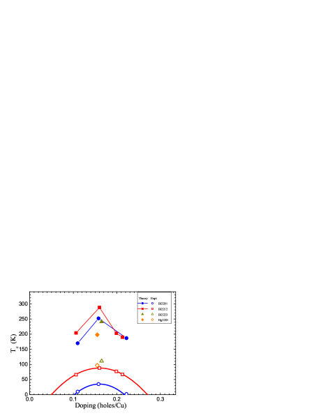
Figure 3: Experimental critical temperature (open symbols) and $T_{c}$’s calculated in the Eliashberg formalism (closed symbols) using the experimentally measured $\tilde{\Pi}(\omega)$ of Fig. 2 at 290 Kelvin as input parameters.

We take this analysis a step further by calculating $T_{c}$ from the glue spectra below 100 meV ($\tilde{\Pi}_{pk}$ ) and above 100 meV ($\tilde{\Pi}_{cnt}$). The resulting coupling constants and $T_{c}$’s are indicated in Table 1. On the underdoped side $\tilde{\Pi}_{cnt}$ vanishes, and $T_{c}$ is given only by the coupling to the intense 50-60 meV peak in $\tilde{\Pi}(\omega)$, but in this doping range we have to be careful with the interpretation of our results. As mentioned in the introduction our $\tilde{\Pi}(\omega)$ spectra represent effective coupling functions, which may contain effects arising from features not captured by the strong coupling equations 1 and 3. If, for example, a pseudogap opens in the electronic spectrum this will affect the shape of $\tilde{\Pi}(\omega)$. These effects likely play a role for the underdoped samples, but are not expected to affect much the room temperature values, indicated in Table 1 and Fig. 3. On the contrary, the larger temperature dependence seen for underdoped samples in Fig. 2 may well be a result of the opening of a pseudogap. For the overdoped samples the $T_{c}$’s calculated from $\tilde{\Pi}_{pk}$ are smaller than the experimental values. For example, for Bi2212 with the highest doping $\tilde{\Pi}_{pk}$ gives only $T_{c}<20$K, whereas $\tilde{\Pi}_{cnt}$ gives 160 K, implying that the glue-function above 100 meV is of crucial importance for the pairing-mechanism. Since only electronic modes can have such high energies, an important contribution to the high $T_{c}$ mechanism comes apparently from coupling to electronic degrees of freedom, i.e. spinscalapino-PRB-1986 ; millis-PRB-1990 ; maier-PRL-2008 ; norman-PRB-2006 or orbital current fluctuationsvarma-PRL-1989 .

VI Summary

In summary, the $\tilde{\Pi}(\omega)$ spectrum obtained from the optical spectra of 10 different compounds using a strong coupling analysis, is observed to consist of two features: (i) a robust peak in the range of 50 to 60 meV and (ii) a doping dependent continuum extending to 0.3 eV for the samples with the highest $T_{c}$. We perform an important test of the internal consistency of the strong coupling formalism by showing that the temperature dependence of the optical spectra is determined by Fermi and Bose factors in the strong coupling expressions. The remaining temperature dependence of $\tilde{\Pi}(\omega)$ can therefore be taken to indicate that part of the $\tilde{\Pi}(\omega)$ spectrum is electronic in origin. We observe an intriguing correlation between the doping trend of the experimental glue spectra and the critical temperature. Finally we obtain an upper limit to the contribution of electron-phonon coupling to the pairing of the overdoped samples, which is too small to account for the observed critical temperature.

VII Acknowledgments

We gratefully acknowledge C.M. Varma, D.J. Scalapino, J. Zaanen, A.V. Chubukov, C. Berthod, J.C. Davis, and A. Millis for stimulating discussions. This work is supported by the Swiss National Science Foundation through Grant No. 200020-113293 and the National Center of Competence in Research (NCCR) Materials with Novel Electronic Properties MaNEP .

VIII Appendix

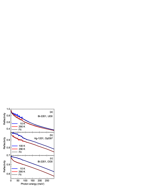
Figure 4: Experimental reflectivity (red and blue lines) and fit curves (black lines) for selected samples and temperatures. (a): underdoped non-superconducting Bi-2201 (UD0). (b): optimally doped Hg-1201 with $T_{c}\approx$ 97 K (OpD97) [heumen-PRB-2007, ] (c): overdoped non-superconducting Bi-2201 (OD0). Weak sharp peaks, particularly visible for the strongly underdoped sample in panel (a) are due to transverse optical phonons, which we do not intend to fit.

The inversion of Eq’s 1 and 2 allows to extract $\tilde{\Pi}(\omega)$ from experimental data of the optical conductivity, or related optical spectra. The accuracy of the resulting $\tilde{\Pi}(\omega)$ spectrum is in practice limited by the convolution with thermal factors expressed by Eq’s 1 and 2 dordevic-PRB-2005 . Microscopic models giving roughly the same $\tilde{\Pi}(\omega)$ spectra, which differ however in the details of the frequency dependence of this quantity, may therefor provide fits to the directly measured optical quantities, such as infrared reflectance spectra, which at first glance look satisfactory, but the remaining discrepancies with the experimental spectra may nevertheless be of significant importance for the proper understanding of the optical data. It is therefore of crucial importance to test the ’robustness’ of each fit with regard to the spectral shape of the $\tilde{\Pi}(\omega)$ function imposed by such models. This robustness can be tested by including in the fit-routine one or several ’oscillators’ superimposed on the model function. When the model glue function provides a complete description of the electronic structure, adding extra oscillators will not result in an improvement of the quality of the fit. We have used this approach to test functional forms commonly used in the literature, in particular the marginal Fermi liquid (MFL) model varma-PRL-1989 and the Millis-Monien-Pines (MMP) representation of the spin fluctuation spectrummillis-PRB-1990 .

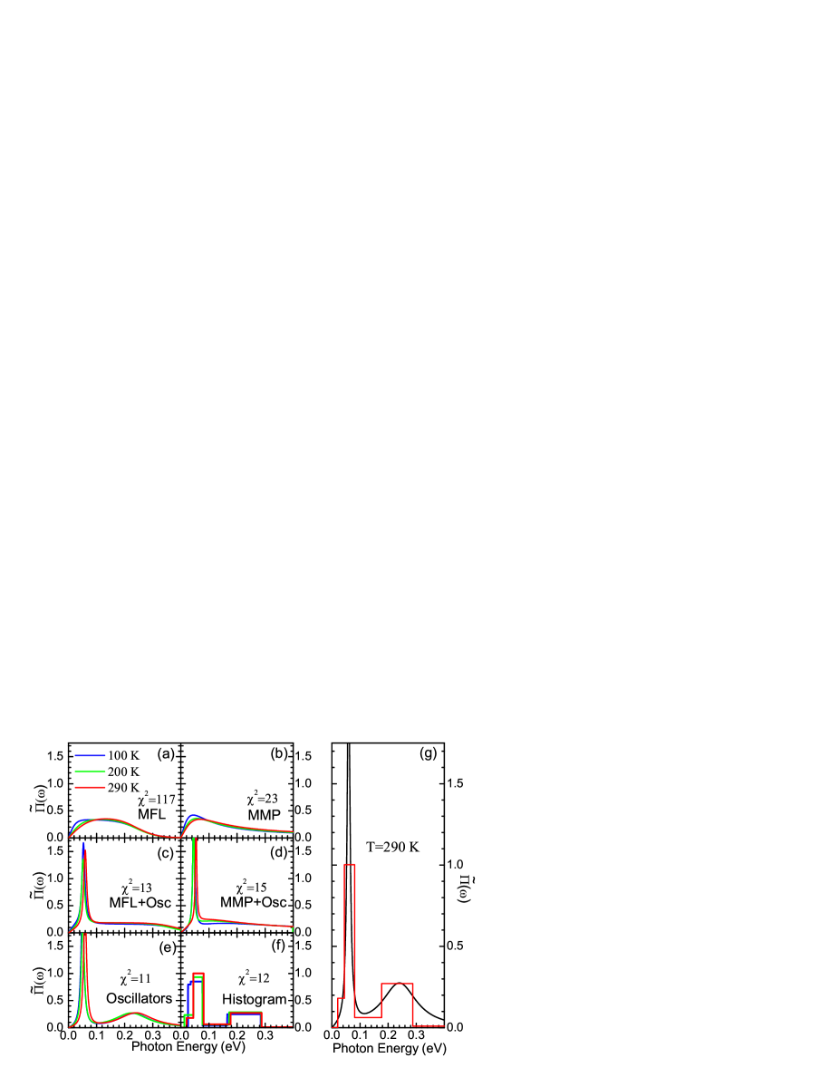
Figure 5: Comparison of several models. The number of data points over which $\chi_{j}^{2}$ is summed (see Eq. 1) is $N=400$. The quoted values of $\chi^{2}$ are those for the room temperature spectra. At 100 K these values increase by a factor 1.5 (MFL) and 3.5 (MMP). In contrast, in the oscillator and the histogram model the $\chi^{2}$ was found to be independent of temperature.

We found that neither of these functional forms describe completely the experimental data. In search of a more flexible form of $\tilde{\Pi}(\omega)$ we used a superposition of lorentzian oscillators and found that it could be used to describe all available experimental data in a consistent manner. The resulting $\tilde{\Pi}(\omega)$ functions and trends are equivalent to those in Fig. 2. From these initial tests we concluded that due to the thermal smearing expressed by Eq’s 1 and 2 our $\tilde{\Pi}(\omega)$ spectra can only be determined with limited resolution. This lead us to the use of a histogram representation, where each block in the histogram represents a likelihood to find coupling to a mode with a well determined coupling strength. For the lowest frequency interval ($0<\omega<\omega_{1}$) a triangular shape was used instead of a block, which is necessary to avoid problems with the convergence of the integral $\lambda=2\int_{0}^{\infty}\omega^{-1}\tilde{\Pi}(\omega)d\omega$. In practice the output generated by the fitting routine has low intensity in this first interval, and the triangles are therefore difficult to distinguish in Fig. 2.

To give an example: The block centered at 55 meV seen in the Hg-1201 sample in Fig. 2 has $\lambda\sim 1$ and a width of about 30 meV. Our histogram representation implies the presence of a coupling to one or several modes between 45 meV and 75 meV with an integrated coupling strength of 1. The histograms thus constitute the most detailed representation of $\tilde{\Pi}(\omega)$ given the precision of our experimental reflectivity and ellipsometry spectra.

Examples of experimental reflectivity data together with the fits are shown in Fig. 4 for a selection of representative data sets spanning the entire doping and temperature range. As the fitted curves are within the limits of the experimental noise, further reduction of $\chi^{2}$, while in principle possible by fitting the statistical noise of the data, can not improve the accuracy of the $\tilde{\Pi}(\omega)$ functions.

Starting from a $\tilde{\Pi}(\omega)$ function we can calculate the optical conductivity, which in turn is fed into standard Fresnel expressions to calculate the experimentally measured quantities, i.e. reflectivity and ellipsometric parameters. The fitting routine is based on the Levenberg-Marquardt algorithm and uses analytical expressions for the partial derivatives of the reflectivity coefficient $R$, and the ellipsometric parameters $\psi$ and $\Delta$ relative to the parameters describing the $\tilde{\Pi}(\omega)$ function. The algorithm is based on minimizing a functional $\chi^{2}$ which is given by,

$$\chi^{2}=\sum_{i=1}^{N}\left(\frac{R(\omega_{i})-f(\omega_{i},p_{1},...,p_{n})}{\sigma_{i}}\right)^{2}$$ (7)

where $R(\omega_{i})$ is an experimentally measured datapoint, $f(\omega_{i},p_{1},...,p_{n})$ is the calculated value in this point based on parameters $p_{1},...,p_{n}$ and the difference between these two is weighed by the errorbar $\sigma_{i}$ determined for $R(\omega_{i})$. For a given set of reflectivity and ellipsometry data at one particular temperature, using a standard PC, the iteration takes about 3 hours until convergence is reached. The Levenberg-Marquardt least squares method is an extremely powerful method to find the minimum of $\chi^{2}$ in a multidimensional parameter space. To ensure that $\chi^{2}$ has converged to the global minimum in parameter space several tests have been performed, for each individual sample and temperature displayed in Fig. 5, where in each test the optimization process was started from a different set of starting parameters. To give some idea of the robustness of our method we will here discuss one representative example: optimally doped Hg-1201.

The models are evaluated based on the minimum found for $\chi^{2}$. A comparison of Fig. 5 (a-d) shows that the MMP model describes better the optical data then the MFL model but that they give similar results if we add an extra oscillator to these models. Panels 5 (e-f) show the model independent results mentioned above and are very similar to the modified MMP and MFL model. The models in these last two panels have the same $\chi^{2}$ and the comparison in Fig. 5g shows that the histogram representation realistically expresses the uncertainty in the position of the low energy peak, while the correspondence between the features in both models remains excellent. It is interesting that the model with two oscillators is described by 6 parameters, while the histogram representation uses 12 parameters. The fact that the fit-routine adjusts the latter 12 parameters in such a manner as to reproduce the two oscillators, proves that the features represented in the righthand panel of Fig. 5 are realistic.

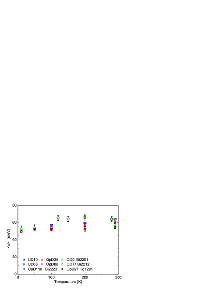
Figure 6: Temperature dependence of $\left<\omega\right>$ for the $\tilde{\Pi}(\omega)$ spectra presented in figure 2. The error bars are defined in Eq. 9.

The models presented in figure 5 allow us to make an estimate of the uncertainty in the determination of the frequency of the low energy peak. We define the first moment of this peak as,

$$\left<\omega\right>=\int_{0}^{100meV}\omega\tilde{\Pi}(\omega)d\omega\left/\int_{0}^{100meV}\tilde{\Pi}(\omega)d\omega.\right.$$ (8)

The variance of $\left<\omega\right>$ is defined as,

$$\sigma^{2}=\frac{1}{N}\sum_{i=1}^{N}\left(\left<\omega_{i}\right>-\bar{\left<\omega\right>}\right)^{2}$$ (9)

with $\bar{\left<\omega\right>}$ the mean of the moments of the spectra presented in figure 5 and $i=1...N$ runs over the number of spectra used ($N=6$ for each temperature). For the Hg1201 room temperature spectra presented in figure 5a-f we find $\left<\omega\right>\approx$ 60 meV and $\sigma\approx$ 3 meV. This value is approximately the same for all samples. In figure 6 we present the temperature dependence of the first moment of the glue functions presented in figure 2.

References

- (1) D.J. Scalapino, E. Loh, J.E. Hirsch, Phys. Rev. B 34, 8190 (1986).
- (2) C.M. Varma, P.B. Littlewood, S. Schmitt-Rink, E. Abrahams, A.E. Ruckenstein, Phys. Rev. Lett. 63, 1996 (1989).
- (3) A.J. Millis, H. Monien, D. Pines, Phys. Rev. B 42, 167 (1990).
- (4) S.V. Shulga, O.V. Dolgov and E.G. Maksimov, Physica C 178, 266 (1991).
- (5) Ar. Abanov, A.V. Chubukov, J. Schmalian, J. Elec. Spec. Rel. Phen. 117, p129 (2000).
- (6) P. W. Anderson, Science 316, 1705 (2007).
- (7) P. Phillips Ann. Phys. 321, 1634 (2006).
- (8) D. N. Basov,S. I. Woods, A. S. Katz, E. J. Singley, R. C. Dynes, M. Xu, D. G. Hinks, C. C. Homes, and M. Strongin, Science 283, 49-51 (1999).
- (9) H.J.A. Molegraaf, C. Presura, D. van der Marel, P.H. Kes, M. Li, Science 295, 2239 (2002).
- (10) F. Carbone, A. B. Kuzmenko, H. J. A. Molegraaf, E. van Heumen, V. Lukovac, F. Marsiglio, D. van der Marel, K. Haule, G. Kotliar, H. Berger, S. Courjault, P. H. Kes, and M. Li Phys. Rev. B 74, 064510 (2006).
- (11) F. Carbone, A. B. Kuzmenko, H. J. A. Molegraaf, E. van Heumen, E. Giannini, and D. van der Marel, Phys. Rev. B 74, 024502 (2006).
- (12) T. A. Maier, D. Poilblanc, and D. J. Scalapino, Phys. Rev. Lett. 100, 237001 (2008).
- (13) where and are the Bose and Fermi-Dirac distribution functions respectivelypballen-PRB-1971 .
- (14) W. Goetze, P. Woelfle, Phys. Rev. B 6, 1226 (1972).
- (15) An alternative frequently used notation for this memory functiontimusk4 is .
- (16) P.B. Allen, Phys. Rev. B 3, 305, (1971).
- (17) A. Comanac, L. de’ Medici, M. Capone, A.J. Millis, Nature Phys. 4, 287, (2008).
- (18) E. van Heumen, R. Lortz, A.B. Kuzmenko, F. Carbone, D. van der Marel, X. Zhao, G. Yu, Y. Cho, N. Barisic, M. Greven, C.C. Homes, and S. V. Dordevic Phys. Rev. B 75, 054522 (2007).
- (19) M.R. Norman, A.V. Chubukov, Phys. Rev. B 73, 140501(R)(2006).
- (20) E. van Heumen, A.B. Kuzmenko, D. van der Marel, H. Eisaki, and W. Meevasana, unpublished.
- (21) D. van der Marel, H. J. A. Molegraaf, J. Zaanen, Z. Nussinov, F. Carbone, A. Damascelli, H. Eisaki, M. Greven, P. H. Kes, and M. Li, Nature 425, 271 (2003).
- (22) J.L. Tallon, J. W. Loram, G. V. M. Williams, J. R. Cooper, I. R. Fisher, J. D. Johnson, M. P. Staines, and C. Bernhard, phys. stat. sol. (b) 215, 531 (1999).
- (23) J. Hwang, T. Timusk, E. Schachinger, J.P. Carbotte, Phys. Rev. B 75, 144508 (2007).
- (24) J. Hwang, E.J. Nicol, T. Timusk, A. Knigavko, J.P. Carbotte, Phys. Rev. Lett. 98, 207002 (2007).
- (25) P.V. Bogdanov, A. Lanzara, S. A. Kellar, X. J. Zhou, E. D. Lu, W. J. Zheng, G. Gu, J.-I. Shimoyama, K. Kishio, H. Ikeda, R. Yoshizaki, Z. Hussain, and Z. X. Shen, Phys. Rev. Lett. 85, 2581 (2000).
- (26) A. Lanzara, P. V. Bogdanov, X. J. Zhou, S. A. Kellar, D. L. Feng, E. D. Lu, T. Yoshida, H. Eisaki, A. Fujimori, K. Kishio, J.-I. Shimoyama, T. Noda, S. Uchida, Z. Hussain, Z.-X. Shen, Nature 412, 510 (2001).
- (27) W. Meevasana ,N. J. C. Ingle, D. H. Lu, J. R. Shi, F. Baumberger, K. M. Shen, W. S. Lee, T. Cuk, H. Eisaki, T. P. Devereaux, N. Nagaosa, J. Zaanen, and Z.-X. Shen, Phys. Rev. Lett. 96, 157003 (2006).
- (28) J. Lee, K. Fujita, K. McElroy, J. A. Slezak, M. Wang, Y. Aiura, H. Bando, M. Ishikado, T. Masui, J.-X. Zhu, A. V. Balatsky, H. Eisaki, S. Uchida, and J. C. Davis, Nature 442, 546 (2006).
- (29) G. Levy deCastro, C. Berthod, A. Piriou, E. Giannini, and O. Fischer, Phys. Rev. Lett. 101, 267004 (2008)
- (30) J.F. Zasadzinski, L. Ozyuzer, N. Miyakawa, K. E. Gray, D. G. Hinks, and C. Kendziora, Phys. Rev. Lett. 87, 067005 (2001).
- (31) B. Mitrovic, H.G. Zarate and J.P. Carbotte, Phys. Rev. B 29, 184 (1984)
- (32) A.J. Millis, S. Sachdev, and C.M. Varma, Phys. Rev. B 37, 4975 (1988).
- (33) C.S. Owen and D.J. Scalapino, Physica 55, 691 (1971).
- (34) S.V. Dordevic, C. C. Homes, J. J. Tu, T. Valla, M. Strongin, P. D. Johnson, and G. D. Gu, D. N. Basov Phys. Rev. B 71, 104529 (2005).