Cluster Solver for Dynamical Mean-Field Theory with Linear Scaling in Inverse Temperature

Abstract

Dynamical mean-field theory and its cluster extensions provide a very useful approach for examining phase transitions in model Hamiltonians, and, in combination with electronic structure theory, constitute powerful methods to treat strongly correlated materials. The key advantage to the technique is that, unlike competing real-space methods, the sign problem is well controlled in the Hirsch-Fye (HF) quantum Monte Carlo used as an exact cluster solver. However, an important computational bottleneck remains; the HF method scales as the cube of the inverse temperature, $\beta$. This often makes simulations at low temperatures extremely challenging. We present here a new method based on determinant quantum Monte Carlo which scales linearly in $\beta$, with a quadratic term that comes in to play for the number of time slices larger than hundred, and demonstrate that the sign problem is identical to HF.

INTRODUCTION

Quantum Monte Carlo (QMC) methods provide an important methodology for solving for the properties of interacting Fermi systems. In auxiliary field techniques HHS ; blankenbecler81 ; nightingale99 ; silvestrelli93 ; zhang03 ; assaad99 ; tremblay92 , the partition function, $Z=\text{Tr}\ {\rm exp}[-\beta\hat{H}]$ is expressed as a path integral, for example, by discretizing the imaginary time $\beta$ into $L$ intervals of length $\Delta\tau$, and separating the one body (kinetic) and two-body (interaction) terms. The latter are then decoupled through the introduction of a Hirsch-Hubbard-Stratonovich (HHS) field HHS which reduces the problem to a quadratic form. The fermion degrees of freedom can be integrated out analytically, leaving an expression for the partition function which is a sum over the possible configurations of the auxiliary field. For interacting lattice Hamiltonians, such as the Hubbard model, this field depends both upon the spatial site and on the imaginary time coordinate. The sum over configurations is performed stochastically, for example, by suggesting local changes and accepting or rejecting with the Metropolis algorithm. The problem is challenging numerically because the summand is the determinant of a product of matrices, one for each fermion species. The determinant is costly to evaluate, and can also become negative at low temperatures, which constitutes the fermion sign problem loh90 .

There are different ways to represent the matrices. In the determinant quantum Monte Carlo (DQMC) approach blankenbecler81 , the matrices have dimension equal to the number of spatial lattice sites $N_{c}$. The matrices are dense, and involve the product of $L$ sparse matrices. The algorithm scaling, $N_{c}^{3}L$, arises from the need to update $N_{c}L$ field variables at a cost of $N_{c}^{2}$ per update, where advantage is taken of an identity for the inverse and determinants of $N_{c}$-dimensional matrices which differ only by a rank-one change. Simulations with this method can now be done on many hundreds of spatial sites. In situations where particle-hole symmetry prevents a sign problem, for example, the half-filled Hubbard Hamiltonian, one can reach arbitrarily low temperatures. DQMC simulations have proven the existence of long-range antiferromagnetic order in the two-dimensional half-filled Hubbard model  hirsch89 , as well as accurately determined the nature of the spectral function and thermodynamic properties at this density paiva01 ; paris07 .

Alternatively, in the algorithm developed by Hirsch and Fye (HF) hirsch86 for embedded-cluster problems, a larger, sparse matrix of dimension $N_{c}L$ is considered. The advantage of the HF-QMC approach is that the matrices are better conditioned (no product of $L$ matrices is involved) and also they remain positive to much lower temperatures; the sign problem is far less severe in the HF-QMC method. However, because determinants of larger matrices are involved, the HF-QMC algorithm scales as $N_{c}^{3}L^{3}$. For this reason, HF-QMC has seen its most powerful applications within dynamical mean-field theory (DMFT) jarrell92 ; georges96 and its cluster extensions, the dynamical cluster approximation (DCA) hettler:dca , and the cellular dynamical mean-field theory (CDMFT) cdmft for which $N_{c}$ is typically small. In effect, DMFT trades the large lattice sizes $N_{c}$, and $N_{c}^{3}$ scaling of DQMC where spatial correlations can be explored, for the ability to reach much lower temperatures at general fillings at the cost of less real-space information, apart from that obtained from the mean field. DMFT also can directly access phase transitions which can only be inferred from finite-size scaling in DQMC.

In this paper, we describe a hybrid approach which combines some of the virtues of both DQMC and HF-QMC. The key algorithmic improvement is a reduction in the $L^{3}$ HF-QMC scaling to linear in $L$. The importance is that this allows much larger $N_{c}$ to be considered. At the same time, we demonstrate analytically (and confirm numerically) that the fermion sign problem in our hybrid algorithm is precisely the same as in HF-QMC, provided that the coupling to the host is fully taken into account. Thus, as in HF-QMC, we can reach low temperatures at quite general fillings. Our paper is organized as follows. We first introduce the basic formalism, including a proof that the sign problem is unchanged from HF-QMC. We then show results for various physical observables including the quasi-particle weight, local moment, and the Green’s function. We demonstrate that the results of our algorithm converge to the same values as that of a well-developed and tested HF-QMC code. We conclude with a comparison of the scaling properties of our new approach.

FORMALISM

DMFT, DCA, and other cluster extensions such as the CDMFT all map the lattice problem onto an effective cluster embedded in a self-consistently determined effective medium. Here, we will add additional sites to the cluster to emulate the effective medium m_caffarel_94 ; embedded . The associated formalism will be sketched for the DMFT and DCA, but it is easily extendable to include CDMFT.

The DCA is a cluster mean-field theory which maps the original $D-$dimensional lattice model onto a periodic cluster of size $N_{c}=L_{c}^{D}$ embedded in a self-consistent host. This mapping is accomplished by replacing the Green’s function and interaction used to calculate irreducible quantities such as the self-energy ($\Sigma$) by their coarse-grained analogs. Spatial correlations up to a range $L_{c}$ are treated explicitly, while those at longer length scales are described at the mean-field level. For details of the DCA formalism and algorithm, please see Ref. maier05 .

The DCA loop converges when the cluster Green’s function equals the coarse-grained Green’s function, ${G_{c}}=\bar{G}$,

$$\bar{G}({\bf{K}},i\omega_{n}) = \frac{N_{c}}{N_{t}}\sum_{\tilde{\bf{k}}}\frac{1}{i\omega_{n}-\epsilon_{\tilde{\bf{k}}+{\bf{K}}}-\Sigma({\bf{K}},i\omega_{n})}$$

$$= \frac{1}{i\omega_{n}-\bar{\epsilon}_{{\bf{K}}}-\Sigma({\bf{K}},i\omega_{n})-\Gamma({\bf{K}},i\omega_{n})},$$

where ${\bf{K}}$ labels a cluster wave number, $\omega_{n}$ is the Matsubara frequency, $\tilde{\bf{k}}$ labels the lattice wave numbers in the Wigner-Seitz cell surrounding ${\bf{K}}$, and $N_{t}$ is the total number of lattice sites. $\bar{\epsilon}_{{\bf{K}}}=N_{c}/N_{t}\sum_{\tilde{\bf{k}}}\epsilon_{\tilde{\bf{k}}+{\bf{K}}}$ is the coarse-grained dispersion and $\Gamma$ is the single-particle hybridization between the DCA cluster and its effective medium.

Here, we consider the two-dimensional (2D) single-band Hubbard model . In order to employ DQMC as a cluster solver, we define an effective cluster Hamiltonian to preserve the coarse-grained Green’s function through the addition of host band degrees of freedom, which we label with $d^{\alpha}$.

$$H = \sum_{{\bf{K}},\sigma}\bar{\epsilon}({\bf{K}})c_{{\bf{K}},\sigma}^{\dagger}c_{{\bf{K}},\sigma}+U\sum_{i}n_{i\uparrow}n_{i\downarrow}$$

$$+ \sum_{{\bf{K}},\sigma,\alpha}\epsilon^{\alpha}({\bf{K}})d_{{\bf{K}},\sigma}^{\alpha\dagger}d_{{\bf{K}},\sigma}^{\alpha}+\sum_{{\bf{K}},\sigma,\alpha}V_{\bf{K}}^{\alpha}c_{{\bf{K}},\sigma}^{\dagger}d_{{\bf{K}},\sigma}^{\alpha}+\text{H.c.}$$

The host band label, $\alpha$, runs from $1$ to $N_{\alpha}$. $\epsilon^{\alpha}({\bf{K}})$ is the dispersion for the $d^{\alpha}$ band, $V_{\bf{K}}^{\alpha}$ is the coupling of the $d^{\alpha}$ band to the $c$ band, $U$ is the strength of the interaction and $n_{i\sigma}=c^{\dagger}_{i\sigma}c_{i\sigma}$ is the number of spin-$\sigma$ electrons on site $i$. Upon integration of the $d-$band degrees of freedom, the correlated band Green’s function becomes

$$G_{\text{eff}}({\bf{K}},i\omega_{n})=\frac{1}{i\omega_{n}-\bar{\epsilon}({\bf{K}})-\Sigma({\bf{K}},i\omega_{n})-\Gamma^{\prime}({\bf{K}},i\omega_{n})},\$$ (3)

where

$$\Gamma^{\prime}({\bf{K}},i\omega_{n})=\sum^{N_{\alpha}}_{\alpha=1}\frac{\left|V_{\bf{K}}^{\alpha}\right|^{2}}{i\omega_{n}-\epsilon^{\alpha}({\bf{K}})}.$$ (4)

The parameters $V_{\bf{K}}^{\alpha}$ and $\epsilon^{\alpha}({\bf{K}})$ are adjusted to fit the DCA or DMFT hybridization function $\Gamma^{\prime}({\bf{K}},i\omega_{n})\approx\Gamma({\bf{K}},i\omega_{n})$. For this, we use Marquardt’s method marquardt to minimize the following merit function at each momentum point:

$$\chi^{2}({\bf{K}})=\sum_{n}\left|\Gamma({\bf{K}},i\omega_{n})-\Gamma^{\prime}({\bf{K}},i\omega_{n})\right|^{2}.$$ (5)

We define the scaled deviation as

$$\eta({\bf{K}})=\frac{\chi({\bf{K}})}{\xi({\bf{K}})}$$ (6)

where $\xi$ is the standard deviation of data.

The discretization of the bath degrees of freedom has been considered in DMFT where exact diagonalization (ED) is used as the Hamiltonian-based impurity solver m_caffarel_94 . Extensions of this method to dynamical cluster mean-field theories have also been largely implemented to study variety of models such as the extended Hubbard or multiband models c_bolech_03 ; c_perroni_07 ; a_liebsch_09 . The advantage of this method is that since ED is essentially exact, there is no systematic error beyond the discretization of the bath. Moreover, more complicated interactions than just the onsite Coulomb can be easily included in the Hamiltonian. However, the disadvantage of ED is that the Hilbert space grows exponentially with the total size of the system, $N_{c}(1+N_{\alpha})$. This greatly limits the size of the clusters that can be studied. This is specially true since (as we discuss below) smaller clusters generally require a higher number of non-interacting bands to fully account for the coupling to the bath, and for larger clusters, e.g., the 16-site cluster, even a very small $N_{\alpha}(=2)$ will make ED inapplicable.

QMC ALGORITHMS AND THE SIGN PROBLEM

The average sign in the DQMC method is equivalent to the average sign in the HF-QMC method in the limit of infinite number of bath bands, $N_{\alpha}\to\infty$. To prove this, we use the path-integral formalism and write the partition function as

$$Z=\int\mathcal{D}[\gamma]\mathcal{D}[\gamma^{*}]e^{-S(\gamma,\gamma^{*})}$$ (7)

where $\mathcal{D}[..]$ denotes the functional integral, $S$ is the action, and $\gamma$ and $\gamma^{*}$ are Grassmann variable vectors. Equation (7) can be approximated by

$$Z\approx\sum_{s_{i,l}=\pm 1}\int\mathcal{D}[\gamma]\mathcal{D}[\gamma^{*}]e^{-S_{0}(\gamma,\gamma^{*})}e^{-S_{I}(\gamma_{c},\gamma_{c}^{*})}$$ (8)

where $S_{(0)I}$ is the (non)interacting part of the action and $\gamma_{c}$ and $\gamma^{*}_{c}$ represent the $c-$band components. In Eq. (8), we have used HHS transformation to decouple the correlation in the interacting part of the action,

$$S_{I}(\gamma_{c},\gamma_{c}^{*})=-\sum_{i,l,\sigma}\lambda\gamma^{*}_{c\ i,l,\sigma}\sigma s_{i,l}\gamma_{c\ i,l-1,\sigma}$$ (9)

Here, $\cosh(\lambda)=e^{\Delta\tau U/2}$, $s_{i,l}$ is the auxiliary field and $l$ is the time index so that $\tau_{\ l}=l\Delta\tau=l\beta/L$. The non-interacting part of the action has the following form:

$$S_{0}(\gamma,\gamma^{*}) = \Delta\tau\sum_{m,l,\sigma}\bigg{[}\gamma^{*}_{m,l,\sigma}\left(\frac{\gamma_{m,l,\sigma}-\gamma_{m,l-1,\sigma}}{\Delta\tau}\right)$$ (10)

$$+ H_{0}(\gamma_{m,l,\sigma},\gamma^{*}_{m,l,\sigma})\bigg{]}$$

where $H_{0}$ is the non-interacting part of the Hamiltonian and $m$ denotes both the spacial coordinate and the band index (including the $c$ band). Equation (8) becomes exact in the limit of $\Delta\tau\rightarrow 0$. By integrating out all the Grassmann variables in Eq. (8), one obtains the following expression:

$$Z\propto\text{Tr}_{\{s_{i,l}\}}\det[G_{\uparrow}^{-1}]\det[G_{\downarrow}^{-1}]$$ (11)

where $G_{\sigma}$ is the Green’s function of size $NL$ with $N=N_{c}+N_{c}N_{\alpha}$.

In the DQMC algorithm, $\Pi_{\sigma}\det[G_{\sigma}^{-1}]$ is used as the sampling weight to complete the sum over the auxiliary field. Note that the action is off-diagonal in time, except for the first term of the non-interacting action which is equal to one along the diagonal [see Eq. (10)]. Therefore, $G_{\sigma}^{-1}$ is an off-diagonal sparse matrix with identity matrices along the diagonal and its determinant can be evaluated from a smaller matrix of size $N$, using the following identity:

$$\det[G_{\sigma}^{-1}]=\det[I+B_{\sigma,L}B_{\sigma,L-1}\dots B_{\sigma,2}B_{\sigma,1}]$$ (12)

where $B_{\sigma,l}$ is the corresponding off-diagonal sub-matrix of $G_{\sigma}^{-1}$ at time slice $l$. The DQMC Markov process proceeds by proposing changes in the HHS fields which are local in space and time, $s_{i,l}\to-s_{i,l}$. Because of that, the ratio of the fermion determinants can be calculated directly from just the diagonal entry of the Green’s function. Similarly, the update of the Green’s function following an accepted move does not require a full $\mathcal{O}(N^{3})$ matrix inversion, but can be done in $\mathcal{O}(N^{2})$ operations. More details about this algorithm can be found in Ref. blankenbecler81 .

Now suppose that instead of integrating out all the Grassmann variables in Eq. (8), we integrate out only the ones associated with the non-interacting electron bands. The partition function can then be written as

$$Z\propto\sum_{s_{i,l}=\pm 1}\int\mathcal{D}[\gamma_{c}]\mathcal{D}[\gamma_{c}^{*}]e^{-S_{c}(\gamma_{c},\gamma_{c}^{*})}$$ (13)

where

$$S_{c}(\gamma_{c},\gamma_{c}^{*})=\sum_{i,l,j,l^{\prime},\sigma}\gamma^{*}_{ci,l,\sigma}\mathcal{G}^{-1}(i,l;j,l^{\prime})\gamma_{cj,l^{\prime},\sigma}+S_{I}(\gamma_{c},\gamma_{c}^{*}).$$ (14)

In the above equation, $\mathcal{G}$ is the non-interacting Green’s function on the cluster ($\mathcal{G}^{-1}=G_{\text{eff}}^{-1}+\Sigma$) whose Fourier transform to momentum and frequency space can be written as

$$\mathcal{G}({\bf{K}},i\omega_{n})=(i\omega_{n}-\bar{\epsilon}_{{\bf{K}}}-\Gamma^{\prime}({\bf{K}},i\omega_{n}))^{-1}.$$ (15)

In the limit of an infinite number of non-interacting host bands, $N_{\alpha}\to\infty$, the self-consistent DCA hybridization function may be exactly represented by the analytic form of Eq. (4), $\Gamma^{\prime}({\bf{K}},i\omega_{n})=\Gamma({\bf{K}},i\omega_{n})$. Therefore, $\mathcal{G}$ will be equal to the DCA cluster-excluded Green’s function, $(\bar{G}^{-1}+\Sigma)^{-1}$. By integrating out the rest of Grassmann variables in Eq. (13), the partition function reads

$$Z\propto\text{Tr}_{\{s_{i,l}\}}\det[G_{c\uparrow}^{-1}]\det[G_{c\downarrow}^{-1}]$$ (16)

where $G_{c}$ is the DCA cluster Green’s function of size $N_{c}L$.

In HF-QMC, to complete the sum over the auxiliary field, $\Pi_{\sigma}\det G_{c\sigma}^{-1}$ is used as the sampling weight. Unlike DQMC, where the inverse Green’s function is sparse, here $G_{c}^{-1}$ is a dense matrix with a dimension that grows with the number of time slices. The HF-QMC Markov process proceeds by proposing local changes in the HHS fields, $s_{i,l}\to-s_{i,l}$. The cost to propose a change, i.e., to calculate the ratio of determinants [Eq. (16)], is low and does not depend upon $L$ or $N_{c}$. If a change is accepted, then the cluster Green’s function matrix $G_{c}$ must be updated. It is possible to write this step as a rank-one matrix update. However, since the inverse Green’s function matrix is dense, it is not possible to decompose it into $N_{c}\times N_{c}$ blocks similar to what was done above with DQMC.

By comparing Eqs. (11) and (16), one can write the following equation for a particular field configuration:

$$C\det[G_{c\uparrow}^{-1}]\det[G_{c\downarrow}^{-1}]=\det[G_{\uparrow}^{-1}]\det[G_{\downarrow}^{-1}].$$ (17)

Since $C$ is independent of fields, the ratio of sampling weights will be the same and therefore, the measured quantities, including the average sign, will have the same statistics in DQMC and HF-QMC algorithms.

RESULTS

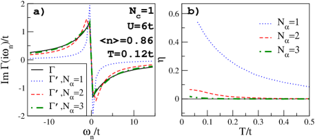
Figure 1: (Color online) (a) The imaginary part of the DMFT hybridization function and fits to its analytic form of the effective cluster problem [Eq. (4)] for $N_{\alpha}=1,2$, and $3$ versus Matsubara frequency. (b) The corresponding scaled deviations of the fits [Eq. (6)] versus temperature.

We apply this method to the 2D Hubbard model [Eq. (FORMALISM)] on a square lattice with nearest-neighbor hopping, $t$, and show results for $\Delta\tau t=1/4$ and the interaction equal to three quarters of the bandwidth ($U=6t$) at filling, $\left<n\right>=0.86$, throughout this paper; calculations at different doping regions and for interaction strength equal to the bandwidth lead to the same trends for the quantities discussed in this work . The quality of the fit of the effective cluster hybridization function [Eq. (4)] to the DCA or DMFT hybridization function, $\Gamma$, is improved by increasing the number of non-interacting bath bands. In Fig. 1(a), we show the imaginary part of $\Gamma(i\omega_{n})$ and the corresponding data for $\Gamma^{\prime}(i\omega_{n})$ from the fitting algorithm using different values of $N_{\alpha}$ for a single impurity problem (DMFT). The improved quality of the fit at a low temperature ($T=0.12t$) can be seen as $N_{\alpha}$ increases from $1$ to $3$. We find that for a finite $N_{\alpha}$, the quality of the fit always decreases as the temperature is lowered. This can be seen in Fig. 1(b) where we show the scaled deviation of the fit [Eq. (6)] for different values of $N_{\alpha}$ as a function of temperature. The hybridization function is poorly fit for $N_{\alpha}=1$ even at high temperatures. However, the scaled deviation is strongly reduced when $N_{\alpha}$ increases.

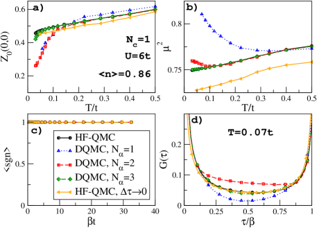
Figure 2: (Color online) The convergence of DQMC to HF-QMC by increasing $N_{\alpha}$ for a single impurity problem (DMFT). We plot (a) the Matsubara frequency quasi-particle fraction versus temperature, (b) the unscreened moment versus temperature, (c) the average sign versus inverse temperature and (d) the Green’s function at a low temperature versus imaginary time, calculated using HF-QMC and DQMC as impurity solvers. For comparison to exact results, a HF-QMC solution with very small $\Delta\tau$ is also presented. For DQMC, we show results for $N_{\alpha}=1,\ 2$, and $3$. For a single-site problem, the average sign is exactly one in all cases. The statistical error bars are smaller than the symbols and are not shown.

As the number of bath degrees of freedom increases, DQMC recovers the HF-QMC results for a single-site problem. We find that a maximum of four bath bands are sufficient for the agreement of the two methods at temperatures as low as $T=0.07t$. This convergence is shown in Fig. 2 for $N_{\alpha}\leq 3$ where we plot the Matsubara frequency quasi-particle weight ($Z_{0}({\bf{K}})=[1-\text{Im}\Sigma({\bf{K}},i\pi T)/\pi T]^{-1}$), local moment ($\mu^{2}=\left<(n_{\sigma}-n_{-\sigma})^{2}\right>$) and the Green’s function, calculated using HF-QMC and DQMC solvers. To have an idea about the absolute errors, we have also included results from an exact solution, i.e., HF-QMC with a very small $\Delta\tau$ ($=1/16t$). We point out that the average fermion sign, shown in Fig. 2(c), is equal to one, regardless of the bath in the single-site limit.

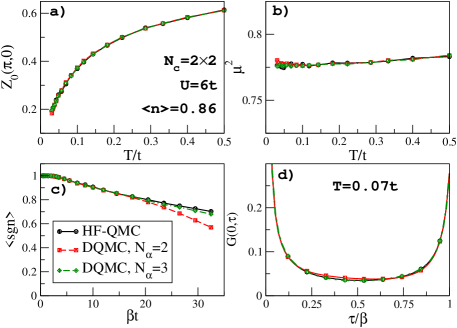
Figure 3: (Color online) Same as Fig. 2 for a $2\times 2$ cluster in the DCA. In (a) and (d), we plot the quasi-particle fraction at ${\bf{K}}=(\pi,0)$ and the Green’s function at the origin, respectively. Results for $N_{\alpha}=1$ cannot be obtained due to a bad sign, even at relatively high temperatures.

The DQMC is a well-behaved cluster solver for the DCA as the number of bath bands needed to recover the HF-QMC results decreases with increasing cluster size. This can be understood from the suppression of the coupling between cluster and host degrees of freedom. In fact, it was shown previously that the hybridization function in the DCA is of order $\mathcal{O}(1/N_{c}^{2/D})$, where $D$ is the dimensionality th_maier_00 . To illustrate that, we plot in Fig. 3 the same quantities of Fig. 2 using the same model parameters but now calculated on a $2\times 2$ cluster. For this cluster, the DQMC results show very good agreement with those of HF-QMC up to $\beta t=34$ when $N_{\alpha}=3$. As proven in the previous section, the average sign in DQMC converges to its HF-QMC value by increasing $N_{\alpha}$ [see Fig. 3(c)]. We find that the sign shows a strong sensitivity to the quality of the hybridization function fit. Thus, when $N_{c}>1$, results for $N_{\alpha}=1$ can not be obtained due to a bad sign problem, even at relatively high temperatures. In Figs. 3(a) and 3(d), we show the quasi-particle fraction at ${\bf{K}}=(\pi,0)$ and the Green’s function at the origin in real space, respectively.

The DQMC cluster solver is best suited for larger cluster simulations where $N_{\alpha}=2$ is sufficient to recover the HF-QMC results. As an example, we present results for a $4\times 4$ cluster in Fig. 4. We find excellent agreement between HF-QMC and DQMC calculations when $N_{\alpha}=2$. Here, the average sign falls more rapidly by decreasing temperature than that of the $2\times 2$ cluster [see Fig. 4(c)]. This limits the calculations for this cluster to $\beta t\leq 15$ in the optimally doped region. However, as can be seen in Fig. 4(c), the average sign is significantly improved from a finite-size DQMC calculation.

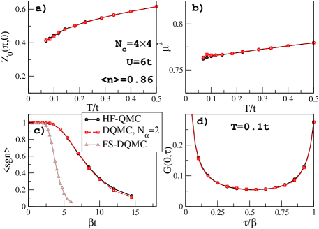
Figure 4: (Color online) Same as Fig. 3 for a $4\times 4$ cluster. For this cluster, the convergence of DQMC to HF-QMC is achieved with $N_{\alpha}=2$. In (c), we also show the average sign for a finite-size (FS) DQMC calculation on this cluster using the same model parameters.

As in HF-QMC, analytic continuation can be performed to calculate real-frequency quantities when DQMC is used as the cluster solver. As an example, we have considered the case of Fig. 4 and calculated the single-particle density of states (DOS) using the maximum entropy method mem . The results indicate that discretizing the bath degrees of freedom does not have a significant influence on the spectra. A comparison between HF-QMC and DQMC DOS has been presented in Fig. 5 where we find that there is a very good agreement between the two density of states in the low energy region. However, there is a slight difference in the high-energy region which would presumably vanish by increasing $N_{\alpha}$.

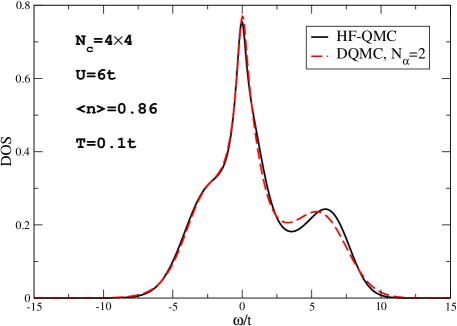
Figure 5: (Color online) Density of states for the case study of Fig. 4. The solid (dashed) line shows the results for HF-QMC (DQMC with $N_{\alpha}=2$).

SCALING

As discussed in previous sections, the linear scaling of the DQMC algorithm with the number of time slices is the main advantage of this cluster solver over HF-QMC. The updating process in HF-QMC, which is the most expensive step in this algorithm, scales like $(N_{c}L)^{3}$. This is a results of $\mathcal{O}(N_{c}L)$ changes in the field variable during each sweep and $\mathcal{O}(N_{c}^{2}L^{2})$ operations to update the Green’s function for each change, using a rank-one updating mechanism. A similar argument applies to the scaling in the DQMC, except that it costs $\mathcal{O}((N_{c}+N_{c}N_{\alpha})^{2})$ to update the inverse Green’s function after each change in the field variable. Since the number of HHS fields and therefore, the number of such updates is proportional to $L$, the overall scaling of updates in DQMC is linear in $L$. The scaling in the system size remains cubic as in other QMC methods and is a big advantage over ED which scales exponentially in the size. To show the linear behavior in $L$, we plot the CPU time for updates versus $L$ on the $4\times 4$ cluster in Fig. 6 (a). First, we compare this to that of HF-QMC for the same model parameters and by setting $\beta t=2.5$. At this fixed $\beta$, the product of matrices in DQMC is stable, which results in a perfectly linear scaling. We find that the updating step in DQMC is up to three orders of magnitude faster than in HF-QMC for a large number of time slices ($L\sim 200$).

In more realistic simulations, increasing $L$ is a consequence of increasing $\beta$ to access low temperatures for a fixed order of systematic error (constant $\Delta\tau$) R_fye1 ; R_fye2 . In this case, we do not expect to see any change in the scaling of HF-QMC. However, in DQMC, an orthogonalization step which scales as $L^{2}$, has to be performed to avoid the round-off errors. To show how the DQMC scaling changes, we also plot in Fig. 6(a), the CPU time for DQMC with $\Delta\tau t=1/16$. We see that the orthogonalization step introduces a quadratic term in $L$ with a coefficient which is two orders of magnitude smaller than the coefficient of the linear term [see diamond symbols in Fig. 6(a)]. This effect on the performance of the algorithm becomes slowly significant only when $L\geq 100$. We point out that measuring the Green’s function in DQMC involves matrix multiplications of the same type as in the updating process, and therefore results in the scaling of the CPU time that is very similar to the one for the updates. However, as can be inferred from Fig. 6(b), measurements generally take more time than updates and the quadratic term appears even in the case of constant $\beta$. The time for measuring the Green’s function in HF-QMC has more or less the same scaling as in DQMC, but is roughly an order of magnitude larger when $L\sim 200$.

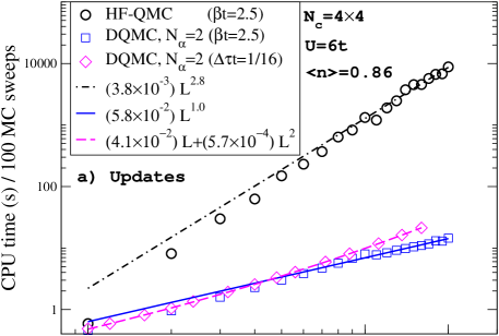
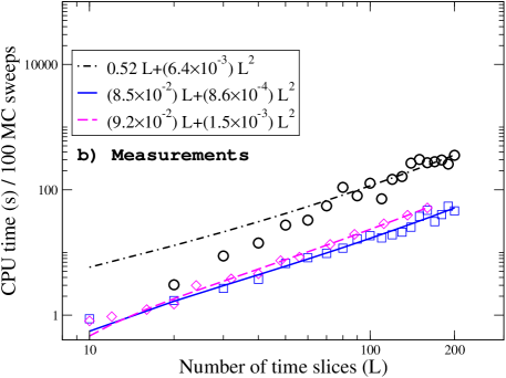
Figure 6: (Color online) The CPU time required for (a) updating and (b) measurement parts of the HF-QMC and DQMC ($N_{\alpha}=2$) algorithms versus the number of time slices on a $4\times 4$ cluster. All other quantities are kept constant. The lines show power-law fits of the data. The diamond symbols show the CPU time in DQMC with a constant $\Delta\tau$ (decreasing temperature) where orthogonalization is performed to stabilize the matrix multiplications.

DISCUSSION

In this paper we have shown that the use of DQMC as a cluster solver provides several order of magnitude speedup over the HF-QMC algorithm, with a sign problem which is well behaved (identical to HF-QMC). This improvement arises from a fundamental reduction in the scaling of the algorithm, from cubic in the inverse temperature, $\beta$, to linear in $\beta$ (with a small quadratic term arising from matrix orthogonalization to reduce round-off errors).

However, the HF-QMC approach itself has already been supplanted in many applications by “continuous time” QMC (CTQMC) algorithms rubtsov ; assaad ; rumbouts ; karlis ; p_werner_06 ; e_gull_07 . We conclude this paper by addressing the relative strengths of the CTQMC technique and the new method presented here. CTQMC eliminates the systematic error inherent in HF-QMC and DQMC, including the method presented here, by stochastically sampling the reducible Feynman graphs of the partition function. Although the matrix sizes are generally smaller than in HF-QMC, the CTQMC algorithm also scales like the cube of the inverse temperature $\beta$ rubtsov . So, DQMC is generally much faster than CTQMC when applied to finite sized systems assaad and also for the embedded cluster problems presented here, especially at low temperatures. However, DQMC has the disadvantage of the introduction of systematic error. These systematic errors in HF-QMC and DQMC may be eliminated by extrapolating the measured quantities in the time step squared, $\Delta\tau^{2}\to 0$ blumer . Since the values of $\Delta\tau$ that are used in this extrapolation are not overly small, the linear in $\beta$ nature of the present algorithm makes for far more efficient calculations, especially at lower temperatures.

CONCLUSIONS

We have developed a DQMC cluster solver for the DMFT, DCA, or CDMFT which scales linearly in the inverse temperature but has the same minus sign problem as HF-QMC. Formally, this is accomplished by defining an effective Hamiltonian for the embedded-cluster problem which includes non-interacting bands for the host. The additional Hamiltonian parameters associated with the bath bands are adjusted to fit the cluster-host hybridization function. We prove that when this fit becomes accurate, this DQMC algorithm recovers the same average sign as HF-QMC. Using DCA simulations of the two-dimensional single-band Hubbard model, we demonstrate that as the number of bath bands increases, we recover the HF-QMC results, including the average sign. The required number of bands is small, increases slightly with lowering temperature, and decreases with increasing cluster size.

References

- (1) R. Blankenbecler, D. J. Scalapino, and R. L. Sugar, Phys. Rev. D 24, 2278 (1981).
- (2) J. E. Hirsch, Phys. Rev. B 28, 4059 (1983).
- (3) L. Chen and A.-M. S. Tremblay, Int. J. Mod. Phys. B 6, 547 (1992).
- (4) P. L. Silvestrelli, S. Baroni, and R. Car, Phys. Rev. Lett. 71, 1148 (1993).
- (5) “Quantum Monte Carlo Methods in Physics and Chemistry” NATO Science Series, Series C: Mathematical and Physical Sciences–Vol 525, edited by M. P. Nightingale and Cyrus J. Umrigar (Kluwer Academic Publishers, New York, 1998)
- (6) F. F. Assaad, Phys. Rev. Lett. 83, 796 (1999).
- (7) S. Zhang and H. Krakauer, Phys. Rev. Lett. 90, 136401 (2003).
- (8) E. Y. Loh, J. E. Gubernatis, R. T. Scalettar, S. R. White, D. J. Scalapino, and R. L. Sugar, Phys. Rev. B 41, 9301 (1990).
- (9) J. E. Hirsch and S. Tang, Phys. Rev. Lett. 62, 591 (1989).
- (10) T. Paiva, R. T. Scalettar, C. Huscroft, and A. K. McMahan, Phys. Rev. B 63, 125116 (2001).
- (11) N. Paris, K. Bouadim, F. Hebert, G. G. Batrouni, and R. T. Scalettar, Phys. Rev. Lett. 98, 046403 (2007).
- (12) J. E. Hirsch and R. M. Fye, Phys. Rev. Lett. 56, 2521 (1986).
- (13) M. Jarrell, Phys. Rev. Lett. 69, 168 (1992)
- (14) A. Georges, G. Kotliar, W. Krauth, and M. Rozenberg, Rev. Mod. Phys. 68, 13 (1996).
- (15) M. H. Hettler, A. N. Tahvildar-Zadeh, M. Jarrell, T. Pruschke, and H. R. Krishnamurthy, Phys. Rev. B 58, R7475 (1998); M. H. Hettler, M. Mukherjee, M. Jarrell, and H. R. Krishnamurthy, Phys. Rev. B 61, 12739 (2000); M. Jarrell, T. Maier, C. Huscroft, and S. Moukouri, Phys. Rev. B 64, 195130 (2001).
- (16) G. Kotliar, S. Y. Savrasov, G. Palsson, and G. Biroli, Phys. Rev. Lett. 87, 186401 (2001)
- (17) M. Caffarel and W. Krauth, Phys. Rev. Lett. 72, 1545 (1994).
- (18) E. Koch, G. Sangiovanni, and O. Gunnarsson, Phys. Rev. B 78, 115102 (2008).
- (19) Th. Maier, M. Jarrell, T. Pruschke, and M. H. Hettler, Rev. Mod. Phys. 77, 1027 (2005).
- (20) For more information about the minimization method please see W. H. Press et. al., “Numerical Recipes in Fortran 77”, 2nd ed. (Cambrige University Press, New York, 2005), p. 678.
- (21) C. J. Bolech, S. S. Kancharla, and G. Kotliar, Phys. Rev. B 67, 075110 (2003).
- (22) C. A. Perroni, H. Ishida, and A. Liebsch, Phys. Rev. B 75, 045125 (2007).
- (23) Ansgar Liebsch and Ning-Hua Tong, Phys. Rev. B 80, 165126 (2009).
- (24) Th. Maier, M. Jarrell, Th. Pruschke, and J. Keller, Eur. Phys. J. B 13, 613 (2000).
- (25) M. Jarrell and J. Gubernatis, Phys. Rep. 269, 133 (1996).
- (26) R. M. Fye, Phys. Rev. B 33, 6271 (1986).
- (27) R. M. Fye and R. T. Scalettar, Phys. Rev. B 36, 3833 (1987).
- (28) K. Mikelsons, A. Macridin and M. Jarrell, Phys. Rev. E 79, 057701 (2009).
- (29) A. N. Rubtsov, V. V. Savkin, and A. I. Lichtenstein, Phys. Rev. B 72, 035122 (2005).
- (30) F. F. Assaad and T. C. Lang, Phys. Rev. B 76, 035116 (2007).
- (31) S. M. A. Rombouts, K. Heyde, and N. Jachowicz, Phys. Rev. Lett. 82, 4155 (1999).
- (32) Philipp Werner, Armin Comanac, Luca dé Medici, Matthias Troyer, and Andrew J. Millis, Phys. Rev. Lett. 97, 076405 (2006).
- (33) Emanuel Gull, Philipp Werner, Andrew Millis, and Matthias Troyer, Phys. Rev. B 76, 235123 (2007).
- (34) N. Blümer, Phys. Rev. B 76, 205120 (2007).