Unwinding in Hopfion vortex bunches

Abstract

We investigate the behaviour of parallel Faddeev-Hopf vortices under energy minimization in a system with physically relevant, but unusual boundary conditions. The homotopy classification is no longer provided by the Hopf invariant, but rather by the set of integer homotopy invariants proposed by Pontrjagin. The nature of these invariants depends on the boundary conditions. A set of tightly wound parallel vortices of the usual Hopfion structure is observed to form a bunch of intertwined vortices or unwind completely, depending on the boundary conditions.

I Introduction

The standard model with knot solitons, the Faddeev-Skyrme (FS) model, was proposed by L. Faddeev in 1975 Faddeev (1975). Since then, many analytical and numerical results have been obtained about this model Vakulenko and Kapitanskii (1979); Kundu and Rybakov (1982); Faddeev and Niemi (1997); Gladikowski and Hellmund (1997); Hietarinta and Salo (1999, 2000); Battye and Sutcliffe (1998, 1999); Sutcliffe (2007). The localized solutions of the FS model are characterized by the Hopf charge, which can be defined if the field is constant at infinity: $\lim_{r\to\infty}\vec{n}(r)=\vec{n}_{\infty}$; this allows one point compactification of the domain $\mathbb{R}^{3}\operatorname{\cup}\{\infty\}\operatorname{\simeq}\mathsf{S}^{3}$ and the definition of Hopf charge using the homotopy group $\pi_{3}(\mathsf{S}^{2})$. However, this is not the only possible boundary condition. Indeed, some physical systems, like rotating superfluid ³He in the $A$ phase Makhlin and Misirpashaev (1995); Ruutu et al. (1994) and certain insulating magnetic materials, called topological insulators Moore et al. (2008), can have different boundary conditions requiring a new topological analysis. There have already been experimental observations of a two dimensional topological insulator in Bi_1-xSb_x, having the topological charge characterized by of $\mathbb{Z}_{2}\times\mathbb{Z}_{2}$ Hsieh et al. (2009).

In this paper we use large scale numerical optimisation routines to investigate the minimum energy configurations of the FS model in novel topological situations. The topological invariants that are relevant when the boundary conditions are no longer the usual $\lim_{r\to\infty}\vec{n}(r)=\vec{n}_{\infty}$ are discussed in section II. It turns out that new topological invariants, introduced by Pontrjagin Pontrjagin (1941), are needed whenever some periodic boundary conditions are used. In section III we describe the Faddeev-Skyrme model and the initial configurations. In Section IV we discuss the process leading to minimum energy configurations from initial configurations consisting of tightly wound and packed vortices parallel to the $z$-direction. We will demonstrate how the topological invariants of section II are conserved while allowing the unwinding of the Hopfion vortices. The behaviour turns out to depend not only on the boundary conditions, but also on the size of the periodic cell as compared to the region occupied by the vortices. Intermediate states of the energy minimization process are used to illustrate the processes that unwind the knot. Locally, these processes are quite similar to those seen in the context of closed Hopfions Hietarinta et al. (2002).

II Topology

We study the FS model in situations where the physical space cannot be compactified to $\mathsf{S}^{3}$ but is periodic in some direction(s). In particular we consider the case when the domain can be identified as $\mathsf{S}^{2}\operatorname{\times}\mathsf{T}^{1}$ (periodic in the $z$-direction) or $\mathsf{T}^{3}$ (periodic in all directions). In these cases the field $\vec{n}$ becomes a map $\vec{n}:\mathsf{S}^{2}\operatorname{\times}\mathsf{T}^{1}\to\mathsf{S}^{2}$ or $\vec{n}:\mathsf{T}^{3}\to\mathsf{S}^{2}$, respectively. Here we differentiate between $\mathsf{S}^{1}$ and $\mathsf{T}^{1}$: If there is a special point $x^{*}$ such that $f(x^{*})=f(-x^{*})$ (e.g. the point at infinity) we use $\mathsf{S}^{1}$ while if the periodicity can be expressed by $f(x)=f(x+L),\,\forall x$ then we use $\mathsf{T}^{1}$.

Note that computationally, the difference between the three cases above is only that of the boundaries. If we want to model the $\mathsf{S}^{3}$ boundary condition $\lim_{r\to\infty}\vec{n}(r)=\vec{n}_{\infty}$ then in the computational lattice the fields at the edges of the box will be fixed to $\vec{n}_{\infty}$ and no interaction can occur across the edges. Next suppose we use the same initial confinguration, but during minimization we only enforce the periodicity condition $\vec{n}(x_{i}^{max})=\vec{n}(x_{i}^{min})$ for some $i$. If the behavior of the system is such that the values of the field on the edges of the box do not change much the system will behave essentially as it behaves when the $\mathsf{S}^{3}$ boundary condition is used. As we shall see, this is also reflected by the fact that in the $\mathsf{T}^{3}$-case, the homotopy classification of the system is still given by the Hopf invariant even though the domain is not topologically $\mathsf{S}^{3}$. The above systems behave differently only when there is strong interaction across one or more edges of the periodic box.

The homotopy classification of the above cases is more complicated than the usual case of $\mathsf{S}^{3}\to\mathsf{S}^{2}$ and was first proposed by Pontrjagin Pontrjagin (1941). A more modern approach, restricted to closed, connected, oriented 3-manifolds is due to Auckly and Kapitanski Auckly and Kapitanski (2005). We will further restrict their result to maps from $\mathsf{S}^{2}\times\mathsf{T}^{1}$ and $\mathsf{T}^{3}$ to $\mathsf{S}^{2}$. The following geometrical descriptions are due to Kapitanski Kapitanski (2005).

Let $\vec{n}:\mathsf{S}^{2}\times\mathsf{T}^{1}\to\mathsf{S}^{2}$. The topological properties of $\vec{n}$ follow the topological properties of its restrictions $\vec{n}|\mathsf{S}^{2}$ and $\vec{n}|\mathsf{T}^{1}$. If we denote these restrictions by $f$ and $g$, respectively, we have $f:\mathsf{S}^{2}\to\mathsf{S}^{2}$ and $g:\mathsf{T}^{1}\to\mathsf{S}^{2}$. The topological properties of $f$ are described by the usual homotopy classification of maps $\mathsf{S}^{2}\to\mathsf{S}^{2}$, i.e., by $\pi_{2}(\mathsf{S}^{2})$ and therefore the relevant homotopy invariant is $s_{2}\operatorname{\equiv}\deg f\in\mathbb{Z}$. The topology of $g$ is more subtle. It turns out that for each value of $s_{2}$ there is another invariant, here called $s_{1}$, which is defined by the map $g$. It can be shown Kapitanski (2005) that $s_{1}\in\mathbb{Z}_{2s_{2}}$.

As an example, consider the stereographic coordinate $z$ of $\mathsf{S}^{2}$ and the map $\vec{n}:\mathsf{S}^{2}\times\mathsf{T}^{1}\to\mathsf{S}^{2}$ for which $f(z)=z^{m}$, where $m\in\mathbb{N}$. It can be shown Manton and Sutcliffe (2004) that for such a map, $\deg f=m$. Thus $s_{2}$ is the number (with multiplicities) of zeros of $f$, i.e. the number of vortex cores. Now, for a simple vortex $s_{2}=\deg f=1$ and therefore $s_{1}\in\mathbb{Z}_{2}$. Thus, there are two homotopy classes, represented by $ze^{is_{1}\theta}$, where $\theta\in[0,2\pi]$ is the coordinate of $\mathsf{T}^{1}$. The function $g$ now describes how many full turns the $\mathsf{S}^{2}$ is rotated as $\theta$ goes from $0$ to $2\pi$. The domain can be regarded as a set of co-centric $2$-spheres for different values of $\theta$ with the inner- and outermost spheres identified. (If $s_{1}=0$, $g$ is the constant map $\theta\mapsto 0$ and $f(w,\theta)=w,\,\forall\theta$ and there is no rotation.) The full map $\vec{n}:\mathsf{S}^{2}\times\mathsf{T}^{1}\to\mathsf{S}^{2}$ represents an $1$-vortex, where two distinct preimages of points on the target $\mathsf{S}^{2}$ have linking number $H$, that we still call the Hopf invariant, but it is not a homotopy invariant in this case.

Detailed description of how the higher numbers of rotations can in this case be unwound to either $s_{1}=\bar{0}$ or $s_{1}=\bar{1}$ can be found in Kapitanski (2005), but we will not discuss this further. The case $s_{2}=0$ is rather special and is not needed here.

Next, consider $\vec{n}:\mathsf{T}^{3}\to\mathsf{S}^{2}$. According to Pontrjagin Pontrjagin (1941), there are three primary homotopy invariants, $t_{1}$, $t_{2}$ and $t_{3}$. In order to determine the values of $t_{i}$, consider $\vec{n}^{-1}(p)\in\mathsf{T}^{3}$, the preimage of a regular value (under the map $\vec{n}$) $p\in\mathsf{S}^{2}$. By continuity of $\vec{n}$, the preimage is a closed loop and therefore can be represented by a directed path $\gamma:\mathsf{S}^{2}\to\mathsf{T}^{3}$. Now, $\gamma\in\pi_{1}(\mathsf{T}^{3})=\mathbb{Z}\operatorname{\times}\mathbb{Z}\operatorname{\times}\mathbb{Z}$ and each of the invariants $t_{i}$ belong to one of the $\mathbb{Z}$ of $\pi_{1}(\mathsf{T}^{3})$. Visually, $t_{i}$ count the number of times $\gamma$ travels around the respective $\mathsf{T}^{1}$ of the $\mathsf{T}^{3}$ and can be determined as follows: For each $t_{i}$, find all the points (with multiplicities) where $\gamma$ pierces a plane defined by $\hat{e}_{i}$, numbering them with $j\in\mathbb{Z}$. For each of these points, let $\epsilon(j)=+1$ if $\gamma$ is directed in the same direction as $\hat{e}_{i}$ and $\epsilon(j)=-1$ if the directions are opposite. (Note that by “piercing” we mean that the preimage has to go through the plane, not just touch it at a point.) Now, for each $i$, we define $t_{i}:=\sum_{j}\epsilon(j)$.

In the $\vec{n}:\mathsf{T}^{3}\to\mathsf{S}^{2}$ case there is also a secondary homotopy invariant, which further divides the maps with equal $t_{1}$, $t_{2}$, $t_{3}$. For fixed values of $t_{i}$, one defines $t=\gcd(t_{1},t_{2},t_{3})$ and for each $t$ there is a secondary homotopy invariant, denoted $h_{t}$. If $t\neq 0$, it can be shown that $h_{t}\in\mathbb{Z}_{2t}$ Auckly and Kapitanski (2005); Kapitanski (2005), and thus for fixed $t_{i}$ and $t>0$ there are $2t$ different homotopy classes. If $t=0$, this invariant is exactly the Hopf invariant and we denote it by $h_{0}$.

Two homotopic maps $\mathsf{S}^{2}\operatorname{\times}\mathsf{T}^{1}\to\mathsf{S}^{2}$ have the same invariants $s_{i}$ and two homotopic maps $\mathsf{T}^{3}\to\mathsf{S}^{2}$ have the same invariants $t_{i}$ and $h_{t}$, but due to the secondary invariants $s_{1}$ and $h_{t}$, maps with the same $s_{2}$ or $t_{i}$ are not necessarily homotopic. In this work, we only deal with the primary invariants $t_{i}$ and $s_{2}$.

III The Faddeev-Skyrme model

The explicit form of the Lagrangian of the Faddeev-Skyrme model can be written in terms of a unit $3-$vector $\vec{n}$ as

$$\mathcal{L} =c_{2}\partial_{\mu}\vec{n}^{T}\partial^{\mu}\vec{n}+c_{4}F_{\mu\nu}F^{\mu\nu},$$ (1)

$$F_{\mu\nu} =\frac{1}{2}\epsilon_{abc}n^{a}\partial_{\mu}n^{b}\partial_{\nu}n^{c},$$ (2)

where $c_{2}$ and $c_{4}$ are coupling constants. Choosing the usual metric $(+,-,-,-)$ yields the static energy density

$$\mathcal{E}_{FS} \operatorname{\equiv}c_{2}\lVert\operatorname{\nabla}\vec{n}\rVert^{2}+c_{4}\lVert F_{jk}\rVert^{2}.$$ (3)

If one requires the field to have a finite energy in $\mathbb{R}^{3}$, it is necessary to impose the boundary condition

$$\lim_{r\to\infty}\vec{n}(r)=\vec{n}_{\infty}=\text{ constant.}$$ (4)

However, if is the physical space is periodic in one or more dimensions, we have in the periodic direction(s) $x_{i}$ $\vec{n}(x_{i})=\vec{n}(x_{i}+L)$, where $L$ is the length of the periodicity. The space no longer compactifies to $\mathsf{S}^{3}$, but depending on the number of periodic dimensions, it becomes i) $\mathsf{S}^{2}\operatorname{\times}\mathsf{T}^{1}$ if one direction is periodic and the two others have the usual boundary condition Eq. (4), ii) $\mathsf{T}^{2}\operatorname{\times}\mathsf{S}^{1}$, in the case where two directions are periodic, and iii) $\mathsf{T}^{3}$ if all directions are periodic. The homotopy classifications of such fields were introduced in section II. We will not consider case ii) in this work.

The initial configuration of a single vortex is the same as in Hietarinta et al. (2004). Using cylindrical coordinates $\rho,\theta,z$ and two integers $m,n$, the form of the field $\vec{n}$ is

$$\vec{n} =\begin{pmatrix}\sqrt{1-f(\rho)^{2}}\,\cos(m\theta+2\pi nz/L_{z})\\ \sqrt{1-f(\rho)^{2}}\,\sin(m\theta+2\pi nz/L_{z})\\ f(\rho)\end{pmatrix},$$ (5)

where $L_{z}$ is the box length in the $z$-direction and $f$ is just some profile function with $f(0)=-1$ and $f(\rho)=+1$ when $\rho=\infty$, which is then cut into a finite size box.

Case i) with initial states composed of a single straight tigthly wound vortex of (5) was studied in Hietarinta et al. (2004). Those initial states correspond to $s_{2}=1$ and values of the Hopf invariant larger than one. In principle they are homotopic to configurations of lower Hopf invariants, namely $H\in\{0,1\}$, but there is an energy barrier which prevents the unwinding.

In this paper, the initial configurations are such that the preimages of $(0,0,-1)$ are the cores of parallel vortices in the $z$-direction; one such vortex is displayed in Figure 1. The small bend visible in the figure was introduced in order to speed up the minimisation process and does not affect the topology or linking number of the system. Such an initial configuration has $s_{2}=m$ in the case i) and $t_{1}=t_{2}=0$, $t_{3}=m$ in the case iii). In both cases, the linking number of preimages is $mn$. All of these are easy to verify visually.

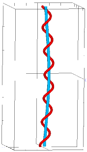
Figure 1: Single vortex in $\mathsf{S}^{2}\times\mathsf{T}^{1}$ or $\mathsf{T}^{3}$ domain. The vortex core $n_{3}=-1$ and one point from the latitude $n_{3}=0.1$ are plotted as narrow blue and red tubes, respectively. The wireframe indicates the boundary of the box.

Vortex bunches are constructed by putting several identical vortices into the computational box, as shown in Figure LABEL:fig:island_initial. For the multi-vortex configurations investigated here, we have used the same values $n=6$ and $m=1$ for each vortex. The value of $n$ may seem rather high, but we have learned in Hietarinta et al. (2004) that for low values the the vortex does not bend much and therefore would not properly interact with the neighboring vortices in the current situation.

In this work, we use the same programs as in Hietarinta and Salo (1999, 2000); Hietarinta et al. (2002, 2004) because the only difference in the computations are the boundary conditions. For numerical computations, this change of boundary conditions is rather minimal, since the MPI library directly supports both periodic and fixed of boundary conditions defined independently for each dimension.

IV Results

We now describe how an initial configuration of a bunch of Hopfion vortices built from Eq. (5) continuously deforms to a minimum energy configuration while conserving the homotopy invariants $s_{i}$, $t_{i}$. We will also describe, how, depending on the details of the initial configuration, the linking number or the Hopfion (the Hopf invariant) is sometimes conserved and sometimes not.

All the computations have used fully periodic boundary conditions, but in different computational lattices.

IV.1 $2\times 2$ vortices in a large box

Let us first consider an initial configuration consisting of $2\times 2$ vortices parallel to the $z$ axis, put into a very large box. It is expected that there would be negligible interaction across the edges of the box, i.e. the system would behave as it would in $\mathsf{S}^{2}\operatorname{\times}\mathsf{T}^{1}$. In the initial configuration, it was necessary to pack the vortices into a tight formation with enough twisting ($n=6$) to ensure that they interact, but not across the boundary. Technically, this was accomplished by building the initial configuration from $16$ narrow boxes: the four central ones contained a single vortex each, while the remaining $12$ pieces were filled with the vacuum, $\vec{n}=(0,0,1)$. In contrast to Hietarinta et al. (2004) we do not fix the field value at the $x,y$ boundary but only require periodicity, this allows us to see whether the behavior of the vortex bunch is the same in $\mathsf{S}^{2}\operatorname{\times}\mathsf{T}^{1}$ and $\mathsf{T}^{2}\operatorname{\times}\mathsf{T}^{1}$, where the $\mathsf{T}^{2}$ is the large box in the $xy$-plane. Indeed, the values on the $xy$-boundaries do not change much during the minimisation process.

The initial configuration is shown in Fig. LABEL:fig:island_initial. Since $\vec{n}_{\infty}=(0,0,1)$, as seen from Eq. (5), the vortex core is at $\vec{n}=(0,0,-1)$. It is easy to count the linking number of preimages, which equals to $24$ (recall that there is a $\frac{1}{2}$ factor involved – there are $48$ crossings) and also the homotopy invariants $t_{i}$: $t_{1}$ and $t_{2}$ are zero (no winding the in $x$- and $y$-directions) and $t_{3}=4$ (four cores pierce the $xy$-plane).

Energy minimisation is applied to the initial configuration using a gradient based algorithm Hietarinta and Salo (1999). Initially, the interaction between vortices is negligible, but after around $40000$ iterations, certain parts of different vortices are close enough to produce evolution which differs from that of a single vortex. At $50000$ iterations, these parts touch and the corresponding preimages reconnect, joining two vortices together. Fig. LABEL:fig:island_touch shows the situation before and LABEL:fig:island_reconnect2 just after the reconnection. The wireframe box showing the initial locations of the vortex cores is also displayed for reference. The reconnection process is allowed because mathematically, the red curve is a single, albeit multiply connected, preimage, and the elementary process is exactly the same as is described in Hietarinta et al. (2002) for a single vortex. Such deformation processes repeat several times in different parts of the lattice until after $300000$ iterations, the initially separate vortices have formed a tangled bunch where the cores (and preimages of a point where $n_{3}=0$) wind around each other (see Fig. LABEL:fig:island_bunch). Visual inspection of the intermediate configurations confirms that, as expected, there is no interaction across the $xy$-boundary. Note that there are six cores (and preimages) piercing the the box at the top and bottom edges, but the direction of one of them is opposite to the others, giving $t_{3}=4$ as required.

(a) fig:island_initial

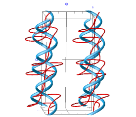
(b)

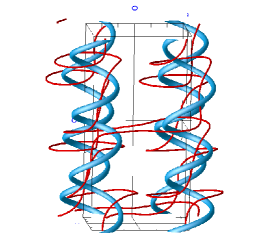
(c)

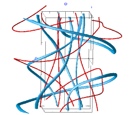
(d)

Figure 2: Relaxation of an initial configuration of four vortices in $\mathsf{S}^{2}\operatorname{\times}\mathsf{T}^{1}$ domain. The colours are as in Fig.  1, but the wireframe now shows the size of the lattice in $z$-direction and the exact locations of the vortex cores (the vertical wires). The computational box is larger and the thicknesses of the tubes are arbitrary.

The final, minimum energy configuration, has the same linking number of preimages and integers $t_{i}$ as the initial state. This is despite the fact that the linking number is no longer guaranteed to be conserved. Its conservation is solely due to the boundaries of the box being very far from the vortices. Indeed, in the next part, we will see that nonconservation is possible.

IV.2 Vortices in a small box

In this case the same initial configuration is put into a box half the previous size, with the expectation that there now would be interaction across the edges of the box. Technically, this was accomplished by taking the same four vortices as above but omitting the $12$ vacuum pieces. Again, the $x,y$-directions are periodic but now the vortices are equally spaced with no change in the spacing at the boundary of the computational box.

The beginning stages of the energy minimization process are identical to that of the large box, but when the vortices start to feel each other the configuration developes in a different manner. Instead of reconnecting to join two vortices together, the reconnected preimages tend to develop into straight filaments extending through the whole periodic lattice. Later, some of the filaments again reconnect and form loops, but since these loops have trivial linking with all other preimages, they can be deformed into nothing.

This is illustrated schematically in Fig. 3, where initially LABEL:sub@fig:schematic_filament_initial, processes familiar from Hietarinta et al. (2002, 2004) have already led to each of the four preimages to split into a relatively straight part parallel to $z$-axis and a loop around it. The preimage loops extend, eventually touching each other, and then reconnect along the dashed curves LABEL:sub@fig:schematic_filament_start_split. Upon further energy minimisation, the filaments will in turn reconnect along the dashed curves to form loops LABEL:sub@fig:schematic_filament_have_split. The resulting loops have trivial linking with other preimages and are threfore free to collapse and vanish LABEL:sub@fig:schematic_filament_ends. The vertical preimages stay relatively unchanged through this process. This is the general mechanism of Hopfion unwinding.

Indeed, the energy minimization process shows how this process of filament and loop formation, followed by the loops shrinking and vanishing, is repeated a number of times in different parts of the computational box so that the final linking number of preimages is zero. The only preimages left in the system are preimages piercing the $xy$-plane. At the same time, the energy approaches the energy of one or more straight unwound vortices.

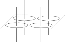
(a)

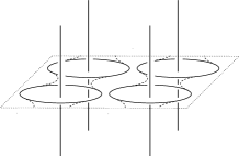
(b)

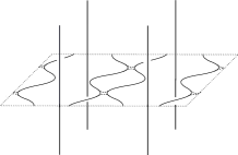
(c)

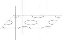
(d)

Figure 3: Schematic illustration of the formation of filaments and contractible loops. The solid and dashed lines represent the preimages and the dotted parallelopiped is the outer boundary of the periodically repeating region containing the four unit cells of the initial vortices.

In order to calculate the invariants $t_{i}$ during the minimisation process, it is necessary to keep track of the directions of the preimages, just as must be done for the computation of the linking number. Now, initially we have $t_{1}=t_{2}=0$ and $t_{3}=4$, so whenever a preimage reaches a boundary of the computational box and pierces it, there must always be a corresponding piercing of the same boundary but in the opposite direction, so that $t_{i}$ are unchanged. Indeed, this has been observed.

In order to further investigate the processes involved in the unwinding of the Hopfion, we simulated a system where the initial condition is a single vortex. Again, we use $m=1$ and $n=6$, but instead of packing several vortices together, we take just one vortex (5) and add no vacuum to the system. The boundary conditions are again fully periodic, but now the length of the period in $xy$-directions is half of that in IV.2. Any splitting and recombination of preimages is now expected to occur across the lattice boundary. This is indeed observed with no new processes present in the system.

V Conclusions

We have studied how the Faddeev-Skyrme model behaves when the domain of the model is taken to be $\mathsf{S}^{2}\operatorname{\times}\mathsf{T}^{1}$ and $\mathsf{T}^{3}$ instead of the usual $\mathsf{S}^{3}$. The new domains require a new homotopy classification which is due to Pontrjagin (1941); Auckly and Kapitanski (2005); Kapitanski (2005). For $\mathsf{S}^{2}\operatorname{\times}\mathsf{T}^{1}$ there is a primary homotopy invariant $s_{2}$ related to the $\mathsf{S}^{2}$ part of the field configuration and when $s_{2}\neq 0$, there is also a secondary invariant $s_{1}$ related to the $\mathsf{T}^{1}$ part. We discuss the invariant $s_{2}$ only and it is seen to be conserved in the energy minimisation process. For $\mathsf{T}^{3}$, there are three primary homotopy invariants, $t_{1}$, $t_{2}$, $t_{3}$ related to the winding numbers around the three tori $\mathsf{T}^{1}$ of the $\mathsf{T}^{3}$. There is a secondary invariant in this case also. When at least one $t_{i}\neq 0$, one defines $t=\gcd(t_{1},t_{2},t_{3})$ and the secondary invariant takes values in $Z_{2t}$. If all $t_{i}=0$, the secondary invariant becomes the Hopf invariant. We have discussed the primary invariants only.

We have constructed a set of initial configurations consisting of a number of twisted vortices where energy minimisation is known to lead to knotted Hopfions in the $\mathsf{S}^{2}\operatorname{\times}\mathsf{T}^{1}$ case Hietarinta et al. (2004). It is observed in this case, that in the continuous deformation driven by energy minimization the conservation of $s_{1}$ and $s_{2}$ does not allow for the unwinding of the knot and leads to an intertwined vortex bunch. In the $\mathsf{T}^{3}$ case neither the conservation of $t_{i}$ nor energy minimisation requires that the knotted structure remains intact and indeed the Hopfion unwinds. The conservation of the homotopy invariants is confirmed by a visual inspection in all cases.

The results have been compared with previously known deformation processes of preimage splitting and reconnecting and found to follow the same deformation “rules” as previously Hietarinta et al. (2002, 2004). No new deformation processes were observed.

The results presented here have possible experimental relevance to the observations of vortices in a rotating superfluid ³He in the $A$ phase Makhlin and Misirpashaev (1995); Ruutu et al. (1994). Another physically relevant situation where maps fron $\mathsf{T}^{3}\to\mathsf{S}^{2}$ arise are insulating magnetic materials in three dimensions, which can have topologically nontrivial properties Moore et al. (2008).