UG-09-05
ENSL-00374319

Twin Supergravities

Diederik Roest ¹ and Henning Samtleben ²

¹ Centre for Theoretical Physics,
University of Groningen,
Nijenborgh 4, 9747 AG Groningen, The Netherlands
d.roest@rug.nl

² Université de Lyon, Laboratoire de Physique,
Ecole Normale Supérieure de Lyon,
46, allée d’Italie, F-69364 Lyon Cedex 07, France
henning.samtleben@ens-lyon.fr

ABSTRACT

We study the phenomenon that pairs of supergravities can have identical bosonic field content but different fermionic extensions. Such twin theories are classified and shown to originate as truncations of a common theory with more supersymmetry. Moreover, we discuss the possible gaugings and scalar potentials of twin theories. This allows to pinpoint to which extent these structures are determined by the purely bosonic structure of the underlying Kac-Moody algebras and where supersymmetry comes to play its role. As an example, we analyze the gaugings of the six-dimensional ${\cal N}=(0,1)$ and ${\cal N}=(2,1)$ theories with identical bosonic sector and explicitly work out their scalar potentials. The discrepancy between the potentials finds a natural explanation within maximal supergravity, in which both theories may be embedded.

1 Introduction

Supersymmetry in general poses strong restrictions on the bosonic and fermionic field content of a theory and the possible interactions between them. A sufficient amount of local supersymmetry even completely fixes the interactions between the different multiplets: the structure of many extended supergravity theories is unique. The only possible deformations are gauge coupling constants and possibly mass parameters. Generically the form of such theories depends on the number of supercharges.

It may therefore come as a surprise that the bosonic sectors of certain specific supergravity theories with different numbers of supersymmetries are in fact identical. In other words, such bosonic sectors allow for different supersymmetric completions. The resulting theories will be referred to as twin supergravities and are the subject of this paper. As such theories have identical bosons but different fermions (and different supersymmetry), they provide an interesting playground to investigate the role of supersymmetry in various aspects. An example of this concerns the BPS sector of these theories. Black holes that are extremal solutions of both twin theories turn out to be BPS in the one theory and non-BPS in the other [1, 2]. That is, the role of BPS and non-BPS sectors are interchanged in the two theories.

In this paper we will study various aspects of twin supergravity theories. First of all, a general classification of twin theories is presented. Secondly, we will discuss how every pair of twin theories originates from a specific supergravity theory, their common parent theory. Finally, we will also address the possible gaugings and resulting scalar potentials of these theories. Turning on a gauging, i.e. promoting part of its global symmetry group to a local gauge symmetry, will introduce a number of additional terms in the bosonic sector of the theory. On the basis of covariance one can show that most of these terms coincide for the two theories. This is not the case for the scalar potential, however. Indeed, one of the main purposes of this paper is to see whether the effect of such gaugings is different in the scalar potentials; in other words, whether the scalar potentials of gauged twin theories ‘feel’ the different fermionic contents of the two theories. One can in fact argue rather convincingly for both possibilities, i.e. different or identical scalar potentials.

An argument supporting the first option is the different amount of supersymmetry of the two theories. In the presence of a gauging, the supersymmetry variations of the fermions acquire additional terms, the so-called fermion shifts that are linear in the gauge coupling constants. The resulting scalar potential takes the form of the difference between the squares of these fermion shifts in order to reconcile the non-abelian deformation with supersymmetry. As the fermionic field content of the two theories is radically different, it is hard to see how their scalar potentials could ever coincide. On the other hand, most gauged supergravities are obtained by Kaluza-Klein reductions on particular backgrounds where the scalar potential is generated from reduction of the bosonic part of the higher-dimensional theory on the non-trivial internal geometry. As these bosonic structures coincide for twin theories, gaugings obtained by Kaluza-Klein reduction will exhibit identical scalar potentials. This illustrates the special nature of twin theories, where arguments based on the bosonic part will lead to different expectations than those based on the fermionic part. In this paper we will analyze the structure of gaugings and resolve this paradox. This issue can have a bearing on the possible connection between supergravities and Kac-Moody algebras, as will be discussed in the conclusions, but also on the possible higher-dimensional origin of gaugings.

This paper is organised as follows. The possible twin theories in supergravity are classified in section 2. Subsequently, in section 3 we show how twin theories can be obtained as truncations of particular theories with more supersymmetry. After a discussion of the general pattern, we illustrate these structures with examples in six and four space-time dimensions. Section 4 addresses the possible gaugings of twin theories using the embedding tensor formalism. We show that these theories admit identical deformations which, however, induce genuinely different scalar potentials. Only for those particular gaugings that can be embedded as gaugings of the common parent theory, the scalar potentials turn out to coincide. We show that these gaugings can be naturally characterized in terms of the quadratic consistency constraints on the embedding tensor of the parent theory. Section 5 discusses the truncation to twin theories with less supersymmetry where similar structures appear. We conclude in section 6 with some discussion on the importance of these findings for the possible connection between supergravities and Kac-Moody algebras. Finally, appendix A contains some more technical details and explicit formulas of the six-dimensional example.

2 Classification of Twin Theories

In this section we will classify the different twin theories, i.e. pairs of supergravities that have the same bosonic field content and interactions amongst them but which can be supersymmetrically extended with fermions in different ways, leading to different amounts ${\cal N}_{\pm}$ of supersymmetry. We choose the notation such that ${\cal N}_{-}<{\cal N}_{+}$. To start with, we focus on the ungauged theories.

${\cal N}=$	${\cal M}_{\rm scalar}=$
$1$	$\rm Riemannian$
$2$	Kähler
$3$	$\rm Quaternionic$
$4$	${\rm Quaternionic}\otimes{\rm Quaternionic}$
$5$	${Sp(2,n)}$	$/$	${Sp(2)\otimes Sp(n)}$
$6$	${SU(4,n)}$	$/$	${SU(4)\otimes SU(n)\times U(1)}$
$8$	${SO(8,n)}$	$/$	$SO(8)\otimes SO(n)$
$9$	${F_{4(-20)}}$	$/$	${SO(9)}$
$10$	${E_{6(-14)}}$	$/$	${SO(10)\otimes SO(2)}$
$12$	${E_{7(-5)}}$	$/$	${SO(12)\otimes SO(3)}$
$16$	${E_{8(+8)}}$	$/$	${SO(16)}$

Table 1: The scalar manifolds ${\cal M}_{\rm scalar}$ of $D=3$ supergravity theories with ${\cal N}$ supercharges.

A useful starting point to identify such twin theories is the classification of $D=3$ supergravity theories [3, *deWit:2003ja]. The reason is that in three dimensions all bosonic fields can be dualized into scalars, such that the bosonic sectors of the various theories are entirely classified by the geometry of their scalar manifolds. This allows for a straightforward comparison. The different scalar manifolds are listen in table 1, where ${\cal N}$ refers to the number of supercharges (in terms of three-dimensional Majorana spinors; maximal supersymmetry thus corresponds to ${\cal N}=16$). The ${\cal N}>4$ theories have symmetric scalar manifolds. For $5\leq{\cal N}\leq 8$ there is the freedom of including a number $n$ of matter multiplets, while for $9\leq{\cal N}\leq 16$ the theories are unique. In contrast, for ${\cal N}\leq 4$ the scalar manifolds are subject to certain geometric conditions and are not necessarily symmetric.

The crucial point for the existence of twin theories is that the geometric conditions on the ${\cal N}_{-}\leq 4$ scalar manifolds also happen to be satisfied by some other theories with a larger ${\cal N}_{+}$. To start with, all supergravity theories with extended supersymmetry have scalar manifolds that are Riemannian and hence can also be interpreted as an ${\cal N}_{-}=1$ theory. Furthermore, the ${\cal N}_{-}=3$ theories have a single quaternionic manifold and hence can also be interpreted as ${\cal N}_{+}=4$ theories with a trivial second factor.

${\cal N}_{-}=$	${\cal N}_{+}=$	${\cal M}_{\rm scalar}=$				$D_{\rm max}=$
$2$	$4$	$SU(2,n)$	$/$	$SU(2)\times SU(n)\times U(1)$	(QK)	$4$
$2$	$6$	$SU(4,n)$	$/$	$SU(4)\times SU(n)\times U(1)$	(K)	$4$
$2$	$8$	$SO(8,2)$	$/$	$SO(8)\times SO(2)$	(K)	$4$
$2$	$10$	$E_{6(-14)}$	$/$	$SO(10)\times SO(2)$	(K)	$4$
$4$	$5$	$Sp(2,1)$	$/$	$Sp(2)\times Sp(1)$	(Q)	$3$
$4$	$6$	$SU(4,2)$	$/$	$SU(4)\times SU(2)\times U(1)$	(QK)	$4$
$4$	$8$	$SO(4,8)$	$/$	$SO(4)\times SO(8)$	(Q)	$6$
$4$	$12$	$E_{7(-5)}$	$/$	$SO(12)\times SU(2)$	(Q)	$6$

Table 2: The twin supergravity theories in three dimensions. ${\cal M}_{\rm scalar}$ denotes the Kähler, quaternionic or quaternionic-Kähler scalar manifold in $D=3$ and $D_{\rm max}$ is the highest dimensions to which these theories can be uplifted.

More interesting are those ${\cal N}_{+}>2$ theories which are described by Kähler (K) manifolds. These can also be interpreted as ${\cal N}_{-}=2$ supergravities. Similarly, there is a number of ${\cal N}_{+}>4$ theories whose bosonic sector is quaternionic (Q). These can therefore be interpreted as an ${\cal N}_{-}=4$ theory. An exhaustive list of these latter twin theories is given in table 2.

A number of comments is in order. First of all, the first example in table 2 with global symmetry group $SU(2,n)$ has either two or four supersymmetries. In this case the scalar manifold is both Kähler and quaternionic (QK). Moreover, the theory with $n=4$ has three possible supersymmetric completions with ${\cal N}=2,4$ or $6$ (in addition to the ${\cal N}=1$ and $3$ possibilities that follow from the previous discussion). Finally, the classification of twin theories in higher dimensions directly follows from that in three dimensions: all higher-dimensional twins are obtained by dimensional oxidation of their $D=3$ counterparts. For instance, the twin theories with highest supersymmetry, i.e. ${\cal N}_{+}=12$ in table 2, can be uplifted to six dimensions. The scalar manifolds of the higher-dimensional oxidations of this theory are listed in table 3.

In this paper we will mainly focus on the twin theories that have ${\cal N}_{-}=4$ in three dimensions, as the twin phenomenon is more striking in cases with higher supersymmetry. Moreover, the structure of the possible gaugings is simpler in these cases, and there is only a corresponding Kac-Moody algebra for theories with at least eight supercharges. In the next two sections we will show how these twin theories have an origin in parent theories with ${\cal N}={\cal N}_{+}+{\cal N}_{-}$ supersymmetries, and discuss their possible gaugings and scalar potentials. We will return to the twin theories with ${\cal N}_{-}=2$ in table 2 in section 5.

$D=$	${\cal N}_{-}=$	${\cal N}_{+}=$	${\cal M}_{\rm scalar}=$
$6$	$(0,1)$	$(2,1)$	$SO(5,1)\times SU(2)$	$/$	$SO(5)\times SU(2)$
$5$	$2$	$6$	$SU^{*}(6)$	$/$	$USp(6)$
$4$	$2$	$6$	$SO^{*}(12)$	$/$	$U(6)$
$3$	$4$	$12$	$E_{7(-5)}$	$/$	$SO(12)\times SU(2)$

Table 3: The twin theories with highest number of supersymmetry in the different dimensions $3\leq D\leq 6$.

3 Parent Theories and Truncations

In the previous section we discussed the pattern of twin supergravities. In particular, in table 2 we identified four different pairs of twin theories with ${\cal N}_{-}=4$ and ${\cal N}_{+}=5,6,8,$ and $12$, respectively. In this section we will show how these twin theories can be obtained by truncation from common parent theories with ${\cal N}={\cal N}_{+}+{\cal N}_{-}=9,10,12,$ and $16$, respectively. The analogous discussion for the four pairs of twins theories with ${\cal N}_{-}=2$ and ${\cal N}_{+}=4,6,8,10,$ respectively, is deferred to section 5.

3.1 General Structure

The starting point of this construction is a supergravity theory (to become the parent theory) with ${\cal N}={\cal N}_{+}+{\cal N}_{-}$ supersymmetries, which has a global symmetry group $\hat{G}$. Two different maximal subgroups of this group will be important in the construction. Firstly, there is the maximal compact subgroup $\hat{H}\subset\hat{G}$, which includes the R-symmetry group of the theory. Secondly, we require the existence of a non-compact maximal subgroup of the type $G\times SU(2)$, such that the groups decompose as

$$\hat{G}~{}\supset~{}G\times SU(2)\,,\qquad\qquad\hat{H}~{}\supset~{}H\times SU(2)\,,$$ (3.1)

where $H$ in turn is the maximal compact subgroup of $G$. The $SU(2)$ factors in (3.1) will be crucial in the truncation, as consistency of the truncation will be based on the representations under this group. Two different consistent truncations of the parent theory are possible. After decomposing its field content with respect to (3.1), we define the truncations

• to keep only those fields that satisfy

  $$(-1)^{F_{SU(2)}}=1\,,$$ (3.2)

  i.e. that transform in a bosonic representation of the $SU(2)$ factor in (3.1), or

• to keep only those fields that satisfy

  $$(-1)^{F_{SU(2)}}(-1)^{F_{\rm space-time}}=1\,,$$ (3.3)

  i.e. space-time bosons that transform in a bosonic representation of the $SU(2)$ factor in (3.1) and space-time fermions that transform in a fermionic representation of it.

These prescriptions define consistent truncations on group-theoretical grounds. For instance, the Lagrangian contains no terms linear in the fields that are truncated out, as it is a bosonic object with respect to both fermion numbers. Similar arguments hold for the supersymmetry variations (i.e. the variation of a field that is truncated out consistently vanishes). Moreover, it is obvious that the two truncations $\mathbb{T}_{\pm}$ give rise to the same bosonic sector but complementary fermionic field content.

Let us consider in detail these truncations for the three-dimensional theories collected in table 1. For the theories with ${\cal N}=16,12,10,$ and $9$, the relevant decompositions (3.1) of the symmetry groups $\hat{G}$ are given by

$${\cal N}=16 : E_{8(8)}~{}\supset~{}E_{7(-5)}\times SU(2)\;,$$

$${\cal N}=12 : E_{7(-5)}~{}\supset~{}SO(4,8)\times SU(2)\;,$$

$${\cal N}=10 : E_{6(-14)}~{}\supset~{}SU(4,2)\times SU(2)\;,$$

$${\cal N}=9 : F_{4(-20)}~{}\supset~{}Sp(2,1)\times SU(2)\;,$$ (3.4)

respectively. Decomposing their field content, and applying the truncation prescription of $\mathbb{T}_{\pm}$, defines the following reductions of the scalar manifolds

$$\frac{E_{8(8)}}{SO(16)} \quad\longrightarrow\quad\frac{E_{7(-5)}}{SO(12)\times SO(3)}~{}\times~{}\frac{SU(2)}{SU(2)}\,,$$

$$\frac{E_{7(-5)}}{SO(12)\times SO(3)} \quad\longrightarrow\quad\frac{SO(4,8)}{SO(4)\times SO(8)}~{}\times~{}\frac{SU(2)}{SU(2)}\,,$$

$$\frac{E_{6(-14)}}{SO(10)\times SO(2)} \quad\longrightarrow\quad\frac{SU(4,2)}{SO(6)\times SO(3)\times SO(2)}~{}\times~{}\frac{SU(2)}{SU(2)}\,,$$

$$\frac{F_{4(-20)}}{SO(9)} \quad\longrightarrow\quad\frac{Sp(2,1)}{SO(5)\times SO(3)}~{}\times~{}\frac{SU(2)}{SU(2)}\,,$$ (3.5)

where the scalars transforming in fermionic representations of $SU(2)$ are truncated out. We recognize as a result the scalar manifolds of the ${\cal N}_{-}=4$ twin theories of table 2. The truncations $\mathbb{T}_{\pm}$ thus define two inequivalent truncations of each of the theories of (3.4) which correspond precisely to the pairs of twins identified in the previous section.

To see this, let us consider the fermionic field content of the theories. In three dimensions, the R-symmetry group is given by the special orthogonal group acting on the $\cal N$ supersymmetries. It is contained in the maximal compact subgroup $\hat{H}$ of the original theory and decomposes under the above prescription as

$$SO({\cal N})\quad\supset\quad SO({\cal N}_{+})\times SU(2)\times{SU(2)}\,,$$ (3.6)

where the second $SU(2)$ factor corresponds to the one displayed in the decomposition of $\hat{H}$ in (3.1), (3.4). The gravitini always transform in the fundamental representation of $SO({\cal N})$ and therefore split up according to

$${\bf\cal N}\quad\longrightarrow\quad({\bf{\bf\cal N}_{+},1,1})\oplus\underline{({\bf 1,2,2})}\,,$$ (3.7)

where we have underlined the fermionic representations with respect to the relevant $SU(2)$. From this decomposition it follows that the truncation $\mathbb{T}_{+}$ preserves ${\cal N}_{+}$ gravitini and thus gives rise to an ${\cal N}_{+}$-extended supergravity. In contrast, the truncation $\mathbb{T}_{-}$ retains the other four gravitini and leads to an ${\cal N}_{-}=4$ theory. Comparing (3.5) to table 2 we have thus shown that (up to possible deformations and gaugings to be discussed in the next section) all pairs of twin theories with ${\cal N}_{-}=4$ can be obtained by consistent truncation of their respective common parent theory.

Note that we have exhibited explicit $SU(2)/SU(2)$ factors on the right hand side of (3.5). Being completely compact these describe no scalar degrees of freedom. In the ${\cal N}_{-}=4$ theory they have the following interpretation. As follows from table 1, three-dimensional ${\cal N}=4$ theories can carry additional hyper-multiplets, consisting of scalars that span a separate quaternionic manifold. The ‘empty’ factor above can be seen to signal the absence of such a manifold, and hence of hyperscalars. Due to this, the $SU(2)$ acts as a global symmetry in the fermionic sector only.

We further note that the decomposition of the group $\hat{G}$ into $G\times SU(2)$ has a simple interpretation in terms of the extended Dynkin diagram. Take the Dynkin diagram of $\hat{G}$ and add one node to obtain the diagram of the (untwisted) affine extension of $\hat{G}$. The semisimple maximal regular subgroups of $\hat{G}$ can be obtained by omitting a single node from this extended Dynkin diagram. The subgroups listed in (3.4) correspond to the elimination of the node to which the affine node is connected. For the first example in (3.4) this is illustrated in figure 1.

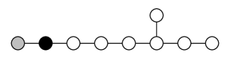
Figure 1: The extended Dynkin diagram of $E_{8(8)}$, where the grey node corresponds to the affine extension and the omission of the black node leads to the relevant semisimple maximal regular subgroup $E_{7(-5)}\times SU(2)$ of $E_{8(8)}$.

We have discussed the truncations in detail in three dimensions, but similar decompositions and truncations can be defined in the higher dimensions; in particular, all higher dimensional examples are obtained by uplift of table 2. For instance, the twin theories with highest amount of supersymmetry, i.e. ${\cal N}_{+}=12$, can be uplifted to six dimensions. The scalar manifolds of the higher-dimensional theories are listed in table 3. In the higher dimensions these twin theories can be obtained similarly by a truncation of maximal supergravity. In this case, the relevant decompositions of the scalar manifolds are

$$\frac{SO(5,5)}{SO(5)\times SO(5)} \quad\longrightarrow\quad\frac{SO(5,1)}{SO(5)}\times\frac{SU(2)}{SU(2)}\times\frac{SU(2)}{SU(2)}\,,$$

$$\frac{E_{6(6)}}{USp(8)} \quad\longrightarrow\quad\frac{SU^{*}(6)}{USp(6)}\times\frac{SU(2)}{SU(2)}\,,$$

$$\frac{E_{7(7)}}{SU(8)} \quad\longrightarrow\quad\frac{SO^{*}(12)}{U(6)}\times\frac{SU(2)}{SU(2)}\,,$$ (3.8)

in dimensions $D=6,5,4$, respectively.

A crucial ingredient for this higher-dimensional construction to work is that the additional $SU(2)$ factor can be interpreted as part of the R-symmetry group in all these dimensions $3\leq D\leq 6$ due to the obvious isomorphisms $SO(3)\sim SU(2)\sim USp(2)$. Furthermore, one can check that in all dimensions these truncations correspond to the maximal regular subgroup that is obtained from the extended Dynkin diagram of $\hat{G}$ as described above. Finally, the particular truncation of the maximal theory in four dimensions was discussed in detail in [7].

3.2 Example in Six Dimensions

It will be useful to illustrate these structures in a concrete example. We will consider the ${\cal N}_{+}=(2,1)$, ${\cal N}_{-}=(0,1)$ twin theories in six dimensions. These can both be obtained from the maximal six-dimensional supergravity with ${\cal N}=(2,2)$ supersymmetry. This parent theory has global symmetry group $\hat{G}=SO(5,5)$ and R-symmetry group $\hat{H}=SO(5)\times SO(5)$. Its bosonic field content is given by 25 scalars parametrizing the coset space $\hat{G}/\hat{H}$, 16 vector fields and 5 antisymmetric tensors. The latter combine together with their magnetic duals into the vector representation ${\bf 10}$ of $SO(5,5)$. Under the decomposition (3.1) with $G=SO(5,1)\times SU(2)$ we obtain the embeddings

$$SO(5,5) \supset SO(5,1)\times SU(2)\times{SU(2)}\,,$$

$$SO(5)\times SO(5) \supset SO(5)\times SU(2)\times{SU(2)}\,.$$ (3.9)

Note that in this case there are in fact two $SU(2)$ factors, of which only the second one will be relevant for the truncation. The bosonic field content of the maximal theory decomposes according to

$$\phi: \quad{\bf 45}\quad \rightarrow\quad ({\bf 1,1,3})\oplus({\bf 1,3,1})\oplus({\bf 15,1,1})\oplus\underline{({\bf 6,2,2})}\,,$$

$$A_{\mu}: \quad{\bf 16}_{c}\quad \rightarrow\quad ({\bf 4,2,1})\oplus\underline{({\bf 4^{\prime},1,2})}\,,$$

$$B_{\mu\nu}: \quad{\bf 10}\quad \rightarrow\quad ({\bf 6,1,1})\oplus\underline{({\bf 1,2,2})}\,,$$ (3.10)

under $SO(5,1)\times SU(2)\times SU(2)\subset SO(5,5)$. The truncations $\mathbb{T}_{\pm}$ eliminate the underlined representations which are fermionic representations under the second $SU(2)$. The scalars here have been given in the adjoint representations. However, as they describe the coset $SO(5,5)/(SO(5)\times SO(5))$, the compact components still need to be modded out. This eliminates the first two components on the right hand side of the first line, while the third component corresponds to the coset $SO(5,1)/SO(5)$ which carries the five physical degrees of freedom. The tensor fields split up in five self-dual and five anti-self-dual components, which together transform in the ${\bf 10}$ representation. After the truncation, five self-dual and one anti-self-dual tensor fields remain. The truncated theory thus does not straightforwardly admit an action (see however the construction of [8]), but can be constructed on the level of the equations of motion along the lines of [9, *Nishino:1986dc, *Nishino:1997ff, *Riccioni:2001bg].

The fermions of the parent theory transform in representations of $SO(5)\times SO(5)$, which under (3.9) decompose as

$$\psi_{\mu}: \quad({\bf 4,1})\oplus({\bf 1,4})\quad \rightarrow\quad ({\bf 4,1,1})\oplus({\bf 1,2,1})\oplus\underline{({\bf 1,1,2})}\,,$$

$$\chi: \quad({\bf 4,5})\oplus({\bf 5,4})\quad \rightarrow\quad ({\bf 4,1,1})\oplus\underline{({\bf 4,2,2})}\oplus\underline{({\bf 5,1,2})}\oplus({\bf 5,2,1})\,,$$ (3.11)

under $SO(5)\times SU(2)\times SU(2)\sim USp(4)\times USp(2)\times USp(2)$. In the fermionic sector, as expected, the truncations $\mathbb{T}_{\pm}$ give a different result. Under $\mathbb{T}_{+}$, the underlined components of (3.11) are eliminated. From the gravitini it is clear that this leads to the unique ${\cal N}_{+}=(2,1)$ supergravity, studied in [13]. The other truncation $\mathbb{T}_{-}$ keeps the complementary fermionic representations, i.e. it keeps only the underlined components of (3.11). This leads to an ${\cal N}_{-}=(0,1)$ supergravity coupling eight vector multiplets and five tensor multiplets to minimal supergravity. Like their bosonic truncation, none of these chiral theories admits an action but they can be constructed on the level of the equations of motion. The entire field content of the ${\cal N}_{+}=(2,1)$ comes in singlets under the second $SU(2)$ factor of (3.9), its symmetry group is thus given by $SO(5,1)\times SU(2)$. In contrast, in the ${\cal N}_{-}=(0,1)$ theory, the second $SU(2)$ factor has a non-trivial action on all fermionic fields.

3.3 Example in Four Dimensions

As a second example, let us consider the pair of twin theories in $D=4$ dimensions with ${\cal N}_{+}=6$, ${\cal N}_{-}=2$ supersymmetries. The ungauged theories are obtained by reduction of the previous example, their common parent theory is again given by maximal supergravity. Various aspects of this truncation were also discussed recently in [7].

Maximal supergravity in four dimensions has a global symmetry group $\hat{G}=E_{7(7)}$, whose maximal compact subgroup is $\hat{H}=SU(8)$. The scalars form the corresponding scalar coset, and can be seen to transform in the adjoint $\bf 133$ of $E_{7(7)}$. Not all of these correspond to physical degrees of freedom. Upon splitting up into $SU(8)$, one finds ${\bf 133}\rightarrow{\bf 63}\oplus{\bf 70}$. The former of these is the adjoint of $SU(8)$ and is projected out due to the coset structure, while the latter representation corresponds to the propagating scalar degrees of freedom. Similarly, the vectors transform in the fundamental $\bf 56$ of $E_{7(7)}$. Under an electric subgroup $SL(8)$ these split into ${\bf 28}\oplus{\bf 28}^{\prime}$, corresponding to the physical vector fields and their magnetic duals, respectively. The gravitini transform in the ${\bf 8}$ and the dilatini in the ${\bf 56}$ of $SU(8)$.

To define the truncations $\mathbb{T}_{\pm}$ to the twin theories we will employ the decomposition (3.1) with $G=SO^{*}(12)$, leading to

$$E_{7(7)}\quad\supset\quad SO^{*}(12)\times{SU(2)}\,,\qquad SU(8)\quad\supset\quad U(6)\times{SU(2)}\,.$$ (3.12)

Under the former decomposition, the $E_{7(7)}$-covariant bosons of maximal supergravity split up into

$$\phi: {\bf 133} \quad\rightarrow\quad({\bf 66},{\bf 1})\oplus({\bf 1},{\bf 3})\oplus\underline{({\bf 32}_{s},{\bf 2})}\,,$$

$$A_{\mu}: {\bf 56} \quad\rightarrow\quad({\bf 32}_{c},{\bf 1})\oplus\underline{({\bf 12},{\bf 2})}\,.$$ (3.13)

Similarly, for the fermionic degrees of freedom we find under the latter decomposition of (3.12),

$$\psi_{\mu}: {\bf 8} \quad\rightarrow\quad({\bf 6},{\bf 1})\oplus\underline{({\bf 1},{\bf 2})}\,,$$

$$\chi: {\bf 56} \quad\rightarrow\quad({\bf 20},{\bf 1})\oplus({\bf 6},{\bf 1})\oplus\underline{({\bf 15},{\bf 2})}\,,$$ (3.14)

of $U(6)\times SU(2)$. The truncations $\mathbb{T}_{\pm}$ remove the underlined representations of (3.13). I.e. the physical vectors of the twin theories together with their magnetic duals transform in the ${\bf 32}_{c}$ of $SO^{*}(12)$. The scalar fields span the truncated coset space

$$\frac{E_{7(7)}}{SU(8)} \quad\longrightarrow\quad\frac{SO^{*}(12)}{U(6)}\times\frac{SU(2)}{SU(2)}\,.$$ (3.15)

In the fermionic sector, the two truncations $\mathbb{T}_{\pm}$ pick out complementary sets from the parent theory. The $\mathbb{T}_{+}$ truncation retains six gravitini and 26 dilatini, leading to the ${\cal N}_{+}=6$ theory. In contrast, the $\mathbb{T}_{-}$ truncations leads to the ${\cal N}_{-}=2$ field content of two gravitini and 30 dilatini, required to fill 15 vector multiplets and the supergravity multiplet. Again, the ${\cal N}_{-}=2$ theory possesses an additional $SU(2)$ symmetry that acts exclusively in the fermionic sector. This symmetry is trivial in the ${\cal N}_{+}=6$ theory.

4 Gaugings and Scalar Potentials

In this section we study the deformations of pairs of twin theories, i.e. the possible gaugings of part of their common global symmetry group. While these are identical deformations in the original bosonic sector of the theory, they will induce different effects in the fermionic sectors of the twin theories. As a result, also the scalar potentials induced by the deformation in the bosonic sector will be found to be genuinely different.

We illustrate the general pattern by means of the two examples we have introduced in the previous section. In particular, we explain how the different potentials of the twin theories are obtained by truncation from their common parent theory.

4.1 Example in Six Dimensions

As a concrete example, let us study the gaugings for the pair of six-dimensional ${\cal N}_{+}=(2,1)$, ${\cal N}_{-}=(0,1)$ twin theories that we have introduced and discussed in section 3.2. Following the general scheme [14, *deWit:2004nw, *Samtleben:2005bp, 17, 18], these gaugings are encoded in a constant embedding tensor $\theta$ which transforms in the tensor product of the dual vector field representation with the adjoint representation of the global symmetry group

$$\theta \subset ({\bf 4}^{\prime},{\bf 2},{\bf 1})\otimes\Big{(}({\bf 15},{\bf 1},{\bf 1})\oplus({\bf 1},{\bf 3},{\bf 1})\Big{)}\;.$$ (4.1)

More explicitly, this tensor projects from the generators $t_{\alpha}$ of the global symmetry group onto the generators $X_{M}$ of the gauge algebra that appear in the minimal couplings to the vector fields

$$D_{\mu} = \partial_{\mu}-gA_{\mu}^{M}\,X_{M}\;,\qquad X_{M}~{}\equiv~{}\theta_{M}{}^{\alpha}\,t_{\alpha}\;.$$ (4.2)

A closer analysis along the lines of [19, *deWit:2008ta] shows that only particular sub-representations in this tensor product are allowed in order to define a consistent hierarchy of non-abelian tensor gauge transformations and thus a consistent gauging:

$$\theta : ({\bf 20},{\bf 2},{\bf 1})\oplus({\bf 4}^{\prime},{\bf 2},{\bf 1})\;.$$ (4.3)

The selection of these subrepresentations within (4.1) is based on purely bosonic arguments and thus independent of the particular fermionic sector of the theory. Nevertheless it turns out that precisely the deformations induced by parameters (4.3) allow for a supersymmetrization with either ${\cal N}_{+}=(2,1)$ or ${\cal N}_{-}=(0,1)$ supersymmetries. The deformation parameters give rise to fermionic mass terms and enter quadratically in the scalar potential. Schematically, in every gauged supergravity the fermionic mass terms are of the form

$${\cal L}_{\rm ferm} = \bar{\psi}A\psi+\bar{\psi}B\chi+\bar{\chi}C\chi\;,$$ (4.4)

where $\psi$ and $\chi$ collectively denote the gravitino and spin-1/2 fields, respectively, and we have suppressed all space-time and internal indices. The tensors $A$, $B$, and $C$ are obtained by dressing the constant tensors (4.3) with the scalar fields. The scalar potential in turn takes the schematic form

$${\cal L}_{\rm pot} = \frac{1}{2{\cal N}}\,\Big{(}{\rm tr}\,B^{2}-\frac{D-1}{2}\,{\rm tr}\,A^{2}\Big{)}\;,$$ (4.5)

where ${\cal N}$ is the number of supersymmetries and $D$ the space-time dimension. Even though the ${\cal N}_{+}=(2,1)$ and the ${\cal N}_{-}=(0,1)$ theory are described by the same set (4.3) of deformation parameters, their different fermionic field content implies a different structure of the respective mass tensors $A$, $B$ in (4.4), and thus a priori a different form of their scalar potentials (4.5). In the rest of this section we discuss the structure of these terms on the level of representations; we give the explicit expressions in appendix A.

The ${\cal N}_{-}=(0,1)$ theory admits an additional class of deformations in which (part of) the second $SU(2)$ factor is gauged by the vector fields. The corresponding couplings are described by an additional component of the embedding tensor

$$\lambda : ({\bf 4}^{\prime},{\bf 2},{\bf 3})\;.$$ (4.6)

As the second $SU(2)$ acts exclusively on the fermions, these parameters remain invisible in the bosonic sector except for their quadratic contribution to the scalar potential. They describe the six-dimensional analogue of the local version of the Fayet-Iliopoulos mechanism of four-dimensional ${\cal N}=1$ supergravity. Accordingly, we will refer to the parameters $\lambda$ as the Fayet-Iliopoulos parameters.

It is instructive to identify the origin of the various deformation parameters (4.3), (4.6) within the maximally supersymmetric parent theory in six dimensions. In this theory, the gaugings are described by an embedding tensor transforming in the ${\bf 144}_{c}$ of $SO(5,5)$ [18]. Under (3.9) this tensor decomposes according to

$$\theta:\quad{\bf 144}_{c} \rightarrow ({\bf 20},{\bf 2},{\bf 1})\oplus({\bf 4}^{\prime},{\bf 2},{\bf 1})\oplus({\bf 4}^{\prime},{\bf 2},{\bf 3})\oplus\underline{({\bf 20}^{\prime},{\bf 1},{\bf 2})}+$$ (4.7)

$$\oplus\underline{({\bf 4},{\bf 1},{\bf 2})}\oplus\underline{({\bf 4},{\bf 3},{\bf 2})}\;,$$

and both truncations $\mathbb{T}_{\pm}$ eliminate the underlined components. The remaining representations are precisely in correspondence with the direct analysis of the twin theories (4.3), (4.6). What is interesting and somewhat unexpected in (4.7) is the fact that the truncation from the maximal theory seems to allow for deformations of the Fayet-Iliopoulos type (4.6) even in the ${\cal N}_{+}=(2,1)$ theory where they have not shown up in the direct analysis (4.3). We will see in the following that these are forbidden by an additional quadratic constraint.

Let us further analyze the structure of deformations of the six-dimensional twin theories. As the fermions in both theories transform under the compact group $SO(5)\times SU(2)\times SU(2)$, the possible fermionic mass tensors (4.4) are obtained from branching the embedding tensor (4.3), (4.6) under this compact group, giving rise to

$$({\bf 20},{\bf 2},{\bf 1})\oplus({\bf 4}^{\prime},{\bf 2},{\bf 1})\oplus({\bf 4}^{\prime},{\bf 2},{\bf 3}) \longrightarrow ({\bf 16,2,1})\oplus 2\cdot({\bf 4,2,1})\oplus({\bf 4,2,3})\;.$$ (4.8)

Comparison to the fermionic field content (3.11) allows to identify the various fermionic mass tensors (4.4) in the two theories:

(4.14)

(4.19)

As a result of (4.8), only two of the various $({\bf 4,2,1})$ blocks are linearly independent, and all $({\bf 16,2,1})$ coincide. The scalar potentials of the two theories thus take the schematic expressions

$$V_{(2,1)} = ({\bf 16,2,1})^{2}+({\bf 4,2,1})^{2}+({\bf 4,2,1})^{2}-({\bf 4,2,1})^{2}\;,$$ (4.20)

$$V_{(0,1)} = ({\bf 4,2,1})^{2}+({\bf 4,2,3})^{2}\;,$$ (4.21)

according to (4.5), the squares denoting singlets under the compact $SO(5)\times SU(2)\times SU(2)$ (cf. (A.12), (A.13) for the explicit expressions). A priori, the potentials induced in the twin theories are thus genuinely different and they furthermore explicitly differ from direct truncation of the potential of the maximal theory $V_{(2,2)}$. In particular, $V_{(0,1)}$ is manifestly positive definite in contrast to the indefinite potential of the ${\cal N}_{+}=(2,1)$ theory. However, as the potentials (4.20), (4.21) are obtained from complementary fermionic mass terms (4.14), (4.19) according to the general relation (4.5), it follows that they are related by the general identity

$$4\,V_{(2,2)} = 3\,V_{(2,1)}+V_{(0,1)}\;,$$ (4.22)

where the ${\cal N}=(2,2)$ scalar potential is understood to be truncated to the scalars of the twin theories. Indeed, this relation can be verified for the explicit expressions (A.9), (A.12), and (A.13).

One of our original questions was the possible discrepancy of the scalar potentials in generic twin theories: do the deformations that act identically in the bosonic sector really give rise to different bosonic scalar potentials, despite the fact that both potentials (4.20), (4.21) are obtained by truncating the same ${\cal N}=(2,2)$ potential of the parent theory to an identical bosonic field content? In order to answer this question we need to further analyze the possible consistency constraints on the deformation parameters. A generic gauging is defined by parameters transforming in the representations (4.3), (4.6) subject to additional quadratic constraints that ensure closure of the gauge algebra. Some (bosonic) algebra shows that for the six-dimensional twin theories, these constraints which are quadratic in the parameters (4.3), (4.6) transform according to

$${\cal Q}^{(\theta\theta)}_{\rm constraint} : 2\cdot({\bf 6},{\bf 1},{\bf 1})\oplus({\bf 6},{\bf 3},{\bf 1})\oplus({\bf 10},{\bf 3},{\bf 1})\oplus({\bf 64},{\bf 1},{\bf 1})\;,$$

$${\cal Q}^{(\lambda,\theta)}_{\rm constraint} : ({\bf 6},{\bf 1},{\bf 3})\oplus({\bf 6},{\bf 3},{\bf 3})\oplus({\bf 10}^{\prime},{\bf 1},{\bf 3})\;,$$ (4.23)

under $SO(5,1)\times SU(2)\times SU(2)$. Here, ${\cal Q}^{(\theta\theta)}_{\rm constraint}$ denotes the constraints bilinear in $\theta$ from (4.3) which are identical in the two twin theories, while ${\cal Q}^{(\lambda,\theta)}_{\rm constraint}$ collects the quadratic constraints of the type $\theta\lambda+\lambda\lambda$ that also contain the parameters (4.6) and are only non-trivial in the ${\cal N}_{-}=(0,1)$ theory. All these constraints imply various quadratic identities among the fermionic mass tensors (4.8) (in particular the so-called supersymmetric Ward identities). Some of these may thus imply non-trivial identities among the different forms (4.20), (4.21) of the scalar potential. However, an explicit breaking of (4.23) under the compact $SO(5)\times SU(2)\times SU(2)$ shows that the only constraints which are singlets under the compact group descend from the $({\bf 6},{\bf 1},{\bf 1})$ and thus do not contain the Fayet-Iliopoulos parameters $\lambda\sim({\bf 4}^{\prime},{\bf 2},{\bf 3})$. As the latter do appear in the ${\cal N}_{-}=(0,1)$ scalar potential but are absent for ${\cal N}_{+}=(2,1)$, there is no way to relate the potentials (4.20) and (4.21) by means of the quadratic constraints and we conclude that the scalar potentials in the ${\cal N}_{+}=(2,1)$ and the ${\cal N}_{-}=(0,1)$ twin theories are in general genuinely different.

In order to understand how nevertheless both potentials, (4.20) and (4.21), descend from the same ${\cal N}=(2,2)$ potential upon identical truncation we need to consider the quadratic consistency constraints analogous to (4.23) in the parent theory. These are quadratic constraints on the embedding tensor in the ${\bf 144}_{c}$ of $SO(5,5)$ which transform as ${\bf 10}\oplus{\bf 126}_{c}\oplus{\bf 320}$ under this group [18]. Breaking these representations down to $SO(5,1)\times SU(2)\times SU(2)$ and comparing to (4.23) shows that there is precisely one additional quadratic constraint

$${\cal Q}^{(\rm max)}_{\rm constraint} : ({\bf 6},{\bf 1},{\bf 1})\;,$$ (4.24)

that survives the truncations $\mathbb{T}_{\pm}$. It gives rise to another quadratic identity among the fermionic mass tensors which explicitly involves the Fayet-Iliopoulos parameters $\lambda^{2}$. As a result, the discrepancy between the two scalar potentials

$$V_{(2,1)}-V_{(0,1)}\;,$$ (4.25)

is a linear combination of the three quadratic consistency constraints contained in (4.23) and (4.24). Only those deformations of the twin theories whose parameters in addition to (4.23) satisfy the constraints (4.24) can be embedded as deformations of the maximally supersymmetric parent theory. For these deformations, the scalar potentials (4.20) and (4.21) coincide despite their seemingly different form. Generic deformations of the ${\cal N}_{+}=(2,1)$ and the ${\cal N}_{-}=(0,1)$ theory on the other hand will only satisfy (4.23) and induce genuinely different scalar potentials.

As we show in appendix A, the singlet part within the extra constraint (4.24) takes the (schematic) form (cf. equation (A.21))

$${\cal Q}^{(\rm max)}_{\rm constraint} = ({\bf 4,2,1})^{2}+({\bf 4,2,3})^{2}\;,$$ (4.26)

and in particular admits only real solutions if the Fayet-Iliopoulos parameters $\lambda$ vanish. The additional constraint therefore excludes these additional deformations of the ${\cal N}_{-}=(0,1)$ theory.

The explicit form of the parameters and constraints discussed in this section are given in appendix A. In particular, the explicit form of the potentials (4.20), (4.21) is given in (A.12) and (A.13), in simplified form in (A.22). The additional quadratic constraint (4.24) from the parent theory by virtue of which the two potentials can be mapped into each other is explicitly given in (A.21).

4.2 Example in Four Dimensions

We return to our second example: the truncation of $D=4$ maximal supergravity to the ${\cal N}_{-}=2$ or ${\cal N}_{+}=6$ twins, described in section 3.3. The pattern of their possible gaugings is very analogous to the previous example and we keep the discussion short. The embedding tensor which encodes the possible gaugings of the maximal theory transforms in the ${\bf 912}$ representation of $E_{7(7)}$ [17]. Under (3.12) it decomposes according to

$$\theta:\quad{\bf 912} \rightarrow ({\bf 352}_{s},{\bf 1})\oplus({\bf 32}_{c},{\bf 3})\oplus\underline{({\bf 220},{\bf 2})}\oplus\underline{({\bf 12},{\bf 2})}\;.$$ (4.27)

of $SO^{*}(12)\times SU(2)$. In both truncations the underlined doublet components are projected out, and we are left with a singlet and a triplet component which we denote as

$$\theta: \;\;({\bf 352}_{s},{\bf 1})\,,\qquad\lambda:\;\;({\bf 32}_{c},{\bf 3})\,.$$ (4.28)

As in the $D=6$ example, these correspond to the deformation parameters present in both twin theories and the Fayet-Iliopoulos parameters of the ${\cal N}_{-}=2$ theory, respectively. The former correspond to a gauging of the $SO^{*}(12)$ global symmetry group while the triplet $\lambda$ corresponds to a gauging of the $SU(2)$ R-symmetry that only affects the ${\cal N}_{-}=2$ fermions.

The quadratic constraints to be imposed on these parameters for consistency of the gauging of the twin theories transform in the representations

$${\cal Q}^{(\theta\theta)}_{\rm constraint} : \quad({\bf 66},{\bf 1})\oplus({\bf 462}_{s},{\bf 1})\oplus({\bf 2079},{\bf 1})\;,$$ (4.29)

$${\cal Q}^{(\lambda,\theta)}_{\rm constraint} : \quad({\bf 1},{\bf 3})\oplus({\bf 66},{\bf 3})\oplus({\bf 495},{\bf 3})\;,$$ (4.30)

analogous to (4.23). Only the second set of constraints involves the Fayet-Iliopoulos parameters.

On the other hand, gaugings of the maximal theory satisfy quadratic constraints in the ${\bf 133}\oplus{\bf 8645}$ of $E_{7(7)}$. Upon truncation according to $\mathbb{T}_{\pm}$ this gives rise to all of (4.30) plus an additional constraint transforming as

$${\cal Q}^{(\rm max)}_{\rm constraint} : ({\bf 66},{\bf 1})\;.$$ (4.31)

I.e.  those gaugings of the twin theories that descend by truncation from the maximal supersymmetric parent theory need to satisfy the additional quadratic constraint (4.31). It is crucial to note that the $({\bf 66},{\bf 1})$ of (4.31) is different from the the corresponding representation in (4.29), it notably contains a contribution $\Gamma^{MN}_{\alpha\beta}\lambda^{\alpha i}\lambda^{\beta i}$ bilinear in the Fayet-Iliopoulos parameters.

The scalar potentials induced by these deformations are obtained from (4.5) upon dressing (4.28) with the scalar fields and breaking the representations down to the compact $U(6)\subset SO^{*}(12)$. This yields the schematic form

$$V_{6} = ({\bf 35,1})^{2}+({\bf 15,1})^{2}+({\bf 105,1})^{2}-({\bf 21,1})^{2}\;,$$ (4.32)

$$V_{2} = ({\bf 15,1})^{2}+({\bf 15,3})^{2}-({\bf 1,3})^{2}\;,$$ (4.33)

see [7] for the explicit expressions. In particular, the $SU(2)$ triplets $({\bf 1,3})$, $({\bf 15,3})$ descend from the Fayet-Iliopoulos parameters $\lambda$. As the only constraint that is bilinear in $\lambda$ and contains a singlet under the compact group $U(6)\times SU(2)$ is the additional constraint (4.31), it follows again that the two potentials (4.32), (4.33) coincide only for those gaugings of the twin theories that descend from a gauging of the maximal theory. In this case the gauge parameters are subject to the additional quadratic constraint (4.31) that goes beyond the quadratic constraints of either of the two twin theories. It would be interesting to study if, in contrast to the six-dimensional case, (4.31) admits solutions with real non-vanishing Fayet-Iliopoulos parameters $\lambda$.

5 Truncation to Twins with Less Supersymmetry

The discussion of the previous two sections has been concerned with twin theories that have ${\cal N}_{-}=4$ supersymmetries in three dimensions. We will now turn to the twin theories that have ${\cal N}_{-}=2$ in three dimensions. As we will see, the situation is similar but also differs in a number of respects from the discussion in sections 3 and 4. We will focus on a specific example, which will highlight all the features of this case.

Our main example will be the uplift of the case with the highest amount of supersymmetry to four dimensions, i.e. the fourth row of table 2. In four dimensions, this pair of theories has ${\cal N}_{-}=1$ and ${\cal N}_{+}=5$ supersymmetry, respectively. Its parent theory therefore has ${\cal N}=6$ and has already been encountered before: it is the four-dimensional example that arises from the $\mathbb{T}_{+}$ truncation of maximal supergravity. Its global symmetry group is $\hat{G}=SO^{*}(12)$ and the maximal compact subgroups is $\hat{H}=U(6)$. The vectors and scalars are in the ${\bf 32}_{c}$ and ${\bf 66}$ of $SO^{*}(12)$, respectively. As before, not all of these correspond to propagating degrees of freedom. The ${\bf 32}_{c}$ combines the 16 physical vectors with their magnetic duals while the physical scalars under $U(6)$ transform according to ${\bf 15}_{+2}\oplus\overline{\bf 15}_{-2}$, where we have included the $U(1)\subset U(6)$ weights. Furthermore the gravitini are in the ${\bf 6}_{+1}$ and the dilatini are in the ${\bf 6}_{-5}\oplus{\bf 20}_{+3}$ of $U(6)$.

To define the truncations in this case, one again considers particular decompositions. The relevant maximal subgroups of $\hat{G}$ and $\hat{H}$ are given by

$$SO^{*}(12)\quad\supset\quad SU(5,1)\times U(1)\,,\qquad U(6)\quad\supset\quad U(5)\times U(1)\,.$$ (5.1)

Under the above, the $SO^{*}(12)$-representations of vectors and scalars split up in

$$A_{\mu}: \quad{\bf 32}_{c}\quad\rightarrow\quad{\bf 20}_{0}\oplus{\bf 6}_{-1}\oplus\overline{\bf 6}_{1}\,,$$

$$\phi: \quad{\bf 66}\quad\rightarrow\quad{\bf 1}_{0}\oplus{\bf 35}_{0}\oplus{\bf 15}_{1}\oplus\overline{\bf 15}_{-1} \quad\,.$$ (5.2)

Similarly, in terms of $U(6)$ and the corresponding decomposition, the fermions split up according to

$$\psi_{\mu}: \quad{\bf 6}_{+1}\quad \rightarrow \quad{\bf 5}_{(1,0)}\oplus{\bf 1}_{(-2,1)}\,,$$

$$\chi: \quad{\bf 6}_{-5}\oplus{\bf 20}_{+3}\quad \rightarrow \quad{\bf 5}_{(-2,-1)}\oplus{\bf 1}_{(-5,0)}\oplus{\bf 10}_{(0,-1)}\oplus\overline{\bf 10}_{(3,0)}\,.$$ (5.3)

Some care needs to be taken in identifying which of the two $U(1)$’s in the decomposition of $\hat{H}$ corresponds to the one in the decomposition of $\hat{G}$ (the other one comes appears in the decomposition of $G$). In the representations above this one corresponds to the latter weight.

For the truncation we define the following conditions with respect to the latter $U(1)$’s in $\hat{G}$ and $\hat{H}$:

• to keep only those fields that have even $U(1)$-weight in (5.1), or

• to keep space-time bosons that have even and space-time fermions have odd $U(1)$-weight in (5.1).

From the decompositions above one can easily infer which field content these truncations induce. They agree in the bosonic field content and pick out complementary sets of fermionic fields. From the gravitini it follows that the $\mathbb{T}_{+}$ truncation leads to the ${\cal N}_{+}=5$ theory, while the $\mathbb{T}_{-}$ truncation gives rise to ${\cal N}_{-}=1$. In the bosonic sector, the ten physical scalars parametrize the coset space $SU(5,1)/U(5)$.

Again it is interesting to consider the effect of the truncation on the embedding tensor and thus on the possible gaugings. As discussed before, the embedding tensor of the ${\cal N}=6$ parent theory transforms in the ${\bf 352}_{s}$ of $SO^{*}(12)$. Under the decomposition above this leads to a number of representations of $SU(5,1)\times U(1)$ with even and odd $U(1)$ charges. Keeping only the former yields

$$\theta: \quad{\bf 70}_{0}\oplus\overline{\bf 70}_{0}\,,\qquad\lambda:\quad{\bf 20}_{0}\,,\qquad\xi:\quad{\bf 6}_{2}\oplus\overline{\bf 6}_{-2}\,.$$ (5.4)

The $\theta$ components form the usual embedding tensor of the ${\cal N}_{+}=5$ theory. The $\lambda$ components can be seen as the additional Fayet-Iliopoulos parameters for the ${\cal N}_{-}=1$ theory which describe a gauging of the $U(1)$ R-symmetry group. In this sense they are similar to the additional components we found in the truncation in section 3. However, the charged components $\xi$ are a new feature of this truncation. To understand the meaning of these additional components we recall that four-dimensional ${\cal N}=1$ theories admit additional supersymmetric deformations that are not related to any gauging but described by a holomorphic superpotential $W$. In this case, the mass tensors $A$ and $B$ of (4.4) are proportional to $W$ and $D_{i}W$, respectively, where $D_{i}$ denotes the Kähler covariant derivative with respect to the five complex coordinates of the scalar target space $SU(5,1)/SU(5)$. Thus $W$ and $D_{i}W$ together precisely fill up a complex ${\bf 6}$ of $SU(5,1)$ corresponding to $\xi$. More precisely, we expect the corresponding gaugings of the parent theory to induce, upon the truncation $\mathbb{T}_{-}$, an ${\cal N}_{-}=1$ theory with holomorphic superpotential $W=\xi^{i}{\cal V}_{i}{}^{6}(\phi)$, where ${\cal V}_{i}{}^{6}(\phi)$ denotes the last column of the $SU(5,1)$ coset representative. It would be interesting to study these theories in more detail, presumably some quadratic constraints will again put strong restrictions on the possible choices of $\lambda$ and $\xi$.

For the other twins the situation is completely analogous to the example discussed above. In all cases the parent theory has ${\cal N}_{+}+{\cal N}_{-}$ supersymmetry and its global symmetry group $\hat{G}$ has a non-semisimple maximal subgroup of the form

$$\hat{G}\quad\supset\quad G\times U(1)\,,\qquad\qquad\hat{H}\quad\supset\quad H\times U(1)\,,$$ (5.5)

where we also have indicated the decomposition of the R-symmetry groups. For instance, the relevant decompositions of $\hat{G}$ and $\hat{H}$ in three dimensions are

$${\cal N}=12: \quad\frac{E_{7(-5)}}{SO(12)\times SO(3)} \quad\rightarrow\quad\frac{E_{6(-14)}}{SO(10)\times SO(2)}\times\frac{U(1)}{U(1)}\,,$$

$${\cal N}=10: \quad\frac{E_{6(-14)}}{SO(10)\times SO(2)} \quad\rightarrow\quad\frac{SO(2,8)}{SO(2)\times SO(8)}\times\frac{U(1)}{U(1)}\,,$$ (5.6)

$${\cal N}=8: \quad\frac{SO(8,2n)}{SO(8)\times SO(2n)} \quad\rightarrow\quad\frac{SU(4,n)}{SO(6)\times SU(n)\times SO(2)}\times\frac{U(1)}{U(1)}\,,$$

$${\cal N}=6: \quad\frac{SU(4,n)}{SO(6)\times SU(n)\times U(1)} \quad\rightarrow\quad\frac{SU(2,n)}{SO(3)\times SU(n)\times U(1)}\times\frac{SU(2)}{SU(2)}\times\frac{U(1)}{U(1)}\,.$$

Note that in the last line we find both an empty $SU(2)$ and a $U(1)$ factor, corresponding to the fact that this theory can be interpreted with ${\cal N}_{+}=4$ or ${\cal N}_{-}=2$, respectively.

In all cases we have checked the truncation of the embedding tensor yields analogous results to the example discussed above. In particular, the parent embedding tensor always splits up in the three types of (5.4): the embedding tensor of the ${\cal N}_{+}$ theory, the Fayet-Iliopoulos terms $\lambda$ of the ${\cal N}_{-}$ theory plus the additional charged components labelled by $\xi$ that we suspect to be related to deformations described by a holomorphic superpotential. The latter generically transform in the fundamental of $G$ and its dual representation.

Again the subgroups of $\hat{G}$ defined in (5.5) correspond to maximal regular subgroups, which are non-semisimple in this case. These can be obtained from the extended Dynkin diagrams by the deletion of two nodes, after which one has to add an extra $U(1)$ factor. The example with the highest amount of supersymmetry in three dimensions, corresponding to the first line in (5.6), is illustrated in figure 2.

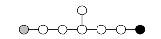
Figure 2: The extended Dynkin diagram of $E_{7(-5)}$, where the grey node corresponds to the affine extension and the omission of the black and the grey node leads to the relevant non-semisimple maximal regular subgroup $E_{6(-14)}\times U(1)$ of $E_{7(-5)}$.

6 Discussion

We have elucidated a number of aspects of twin supergravities — theories with identical bosonic sector but different supersymmetric completion — in particular concerning their gaugings and scalar potentials. We have given a classification of these theories, and shown that in general they descend from truncation of a common parent theory.

Two twin theories allow for the same gaugings parametrised by an embedding tensor, while the ${\cal N}_{-}$-extended theory has the additional possibility to include Fayet-Iliopoulos parameters corresponding to the gauging of symmetries that act exclusively in the fermionic sector. The scalar potentials induced by the gauging in the two theories are genuinely different. They only coincide if the embedding tensor and Fayet-Iliopoulos parameters satisfy an additional quadratic relation that is not required for consistency of the twin theories. The gaugings that satisfy this additional constraint are precisely the ones that can be obtained by truncation from a gauging of the parent theory. Returning to the discussion in the introduction, this shows in particular that gaugings obtained by dimensional reduction (which by construction exhibit the same scalar potential) do satisfy this extra constraint and can be embedded into the parent theory. Gaugings of the twin theories that do not satisfy the additional constraint on the other hand, albeit perfectly viable as supersymmetric gaugings of the twin theories, cannot have a higher-dimensional origin.

Although we have only explicitly demonstrated the relation between the two scalar potentials for our two main examples in six and in four dimensions, we have checked that the same structure in terms of representations of quadratic constraints appears in all other twin cases as well. Hence we expect our conclusions to hold for these cases as well. In the six-dimensional example that we discussed in detail, we found that the additional quadratic constraint implies the Fayet-Iliopoulos parameters to vanish. It is not clear whether this result also holds for the other cases.

In addition to the previous results on twin theories that have ${\cal N}_{-}=4$ in three dimensions, we have also discussed their ${\cal N}_{-}=2$ counterparts. For these theories, an additional component $\xi$ appears in the truncation of the embedding tensor of the parent theory, that is presumably related to deformations described by a particular holomorphic superpotential. As for the Fayet-Iliopoulos parameters it could be that this component in several cases is eliminated due to the quadratic constraints. We leave this for further study.

As alluded to in the introduction, our results on the gaugings and scalar potentials of twin theories may also be relevant for the connection between supergravities and Kac-Moody algebras. Over the last years, the study of supergravity theories has brought up a number of indications that the structure of these theories is to a large extent determined by the underlying higher-rank Kac-Moody algebras [21, *Damour:2002cu]. In particular, many properties that were originally derived from supersymmetry, such as the field content and the possible deformations (mass parameters and gauge coupling constants) of these theories, were later shown to follow from the purely bosonic structure of their global symmetry algebras.

In the case of maximal supergravity [23, *Bergshoeff:2007qi, 25], the decomposition of the adjoint representation of the very extended algebra $E_{11}$ under suitable subgroups reproduces the field content in $D$ dimensions. Moreover, the non-propagating $(D-1)$-forms correspond to the possible deformation parameters of the theories, which were found earlier from compatibility with supersymmetry [14, *deWit:2004nw, *Samtleben:2005bp, 17, 18]. Finally, the non-propagating $D$-forms correspond to the quadratic constraints on these parameters. Likewise, this information turns out to be encoded in the consistency of the non-abelian gauge algebra of the higher-rank $p$-forms in a given dimension [19, *deWit:2008ta, 26, *deWit:2008gc, *Bergshoeff:2009ph, *deWit:2009zv]. A similar picture holds for theories with a lower number of supercharges. Many of these can be associated with a different Kac-Moody algebra, from which the same information can be derived. This was done for the half-maximal supergravities, corresponding to the Kac-Moody extension of $SO(8,8+n)$, in [25]. Similarly, the Kac-Moody algebras for the subset of theories with eight supercharges that have symmetric scalar manifolds were discussed in [30, *Riccioni:2007hm, *Riccioni:2008jz, 33]. A similar analysis can be done for the ‘exceptional’ theories with intermediate amounts of supersymmetry. For theories with less than eight supercharges no corresponding Kac-Moody algebra is known.

This algebraic correspondence raises the question if the underlying very extended Kac-Moody algebras can encode the information about the full theories, including their dynamics and supersymmetric completions. For instance, to date it is not known if and how the form of the scalar potential is encoded in the very extended Kac-Moody algebras (see [34], however). The twin supergravities furnish an interesting test ground for this issue, and the analysis in this paper could help to resolve this point. For instance, the discrepancy between the scalar potentials that we have exhibited could find its origin in the different Kac-Moody algebras associated to the two twin theories: for the ${\cal N}_{+}$-extended theory the associated algebra is the usual Kac-Moody extension of a simple algebra, while for its ${\cal N}_{-}=4$ twin one needs to consider (a quotient of) the Kac-Moody extension of a semisimple algebra [33]. Along a related line of thought, an explicit analysis of the $E_{10}$ $\sigma$-model shows that this yields a positive definite scalar potential, while this is not the case for maximal supergravity in three dimensions [35]. This seems reminiscent of the different scalar potentials (4.20), (4.21) in our six-dimensional example, and may hint at a structure different than maximal supergravity.

Acknowledgements: We are grateful to O. Hohm and M. Trigiante for helpful discussions. The work of D.R. is supported by a VIDI grant from the Netherlands Organisation for Scientific Research (NWO). The work of H.S. is supported in part by the Agence Nationale de la Recherche (ANR).

Appendix

Appendix A Explicit Potentials of the $D=6$ Twin Theories

In this appendix we analyze in detail the example of the six-dimensional ${\cal N}_{+}=(2,1)$, ${\cal N}_{-}=(0,1)$ twin theories embedded into the maximal ${\cal N}=(2,2)$ theory. For the latter theory, we use results and notation from [18]. Its global symmetry group is given by $SO(5,5)$ and the R-symmetry group by the compact $SO(5)\times SO(5)$. Fermionic mass tensors in the maximal theory are described in terms of the embedding tensor, dressed with the scalar fields (4.8). This yields two sets of matrices $T_{\alpha\dot{\alpha}}^{a}$, $T_{\alpha\dot{\alpha}}^{\dot{a}}$ related by the linear constraint

$$\gamma^{a}T^{a}=T^{\dot{a}}\gamma^{\dot{a}}\equiv T\;,$$ (A.1)

with $SO(5)$ gamma matrices $\gamma^{a}$, $\gamma^{\dot{a}}$. Here we use indices $a=1,\dots,5$ and $\alpha=1,\dots,4$ for the vector and the spinor representation, respectively, of the left $SO(5)$ factor of the R-symmetry group, dotted indices refer to the analogous representations of the second $SO(5)$ factor. In matrix notation we suppress the explicit spinor indices.

Explicitly, the relevant fermionic mass terms are given by (see [18] for details)

$${\cal L}_{\rm ferm} = {\textstyle\frac{1}{2}}{\bar{\psi}}_{+\mu}\gamma^{\mu\nu}\,(T)\,\psi_{-\nu}+{\bar{\psi}}_{\mu}\gamma^{\mu}\left(T^{a}-{\textstyle\frac{1}{4}}\gamma^{a}T\right)\chi^{a}+{\bar{\chi}}^{\dot{a}}\left(T^{\dot{a}}+{\textstyle\frac{1}{4}}T\gamma^{\dot{a}}\right)\gamma^{\mu}\psi_{\mu}$$ (A.2)

$$+\dots\;,$$

where dots refer to the $(\chi\chi)$ mass terms that are not relevant for the scalar potential.

In accordance with (4.5), the scalar potential of the maximal theory is given by

$$V_{(2,2)} = \tfrac{1}{8}\,\Big{(}{\rm tr}\left(T^{a}-{\textstyle\frac{1}{4}}\gamma^{a}T\right)^{2}+{\rm tr}\left(T^{\dot{a}}+{\textstyle\frac{1}{4}}T\gamma^{\dot{a}}\right)^{2}-{\textstyle\frac{5}{8}}\,{\rm tr}\,T^{2}\Big{)}$$ (A.3)

$$= \tfrac{1}{8}\,\Big{(}{\rm tr}\left(T^{a}\right)^{2}+{\rm tr}\left(T^{\dot{a}}\right)^{2}-{\rm tr}\,T^{2}\Big{)}\;.$$

Under truncation to the twin theories, and in agreement with (4.8), only the following components of the $T$ tensor survive:

$$T^{a} \rightarrow ({\bf 16,2,1})\oplus({\bf 4,2,1})\;,$$

$$T^{\dot{a}} \rightarrow ({\bf 4,2,1})\oplus({\bf 4,2,1})\oplus({\bf 4,2,3})\;,$$ (A.4)

where only two of the three $({\bf 4,2,1})$ components are linearly independent. More explicitly: breaking the second $SO(5)$ factor of the R-symmetry group according to $SO(5)\rightarrow SU(2)\times SU(2)$ corresponds to a split of indices

$$\dot{\alpha}\rightarrow\{i,\bar{\jmath}\}\;,\qquad\dot{a}\rightarrow\{0,(i,\bar{\jmath})\}\;,$$ (A.5)

with $i,\bar{\jmath}\in\{1,2\}$, corresponding to the branchings ${\bf 4}\rightarrow({\bf\frac{1}{2},0})\oplus({\bf 0,\frac{1}{2}})$ and ${\bf 5}\rightarrow({\bf 0,0})\oplus({\bf\frac{1}{2},\frac{1}{2}})$, respectively. E.g. the tensor $T$ from (A.1) breaks according to

$$T_{\alpha\dot{\alpha}} \rightarrow (T_{\alpha i},T_{\alpha\bar{\imath}})~{}=~{}\left(T^{0}_{\alpha i}-\sqrt{2}\epsilon_{ij}T^{(j,\bar{\jmath})}_{\,\alpha\,\,\bar{\jmath}},-T^{0}_{\alpha\bar{\imath}}-\sqrt{2}\epsilon_{\bar{\imath}\bar{\jmath}}T^{(j,\bar{\jmath})}_{\,\alpha\,\,j}\right)\;.$$ (A.6)

Upon truncation to the twin theories, the second component in truncated out, such that the only non-vanishing component of $T$ is

$$T_{\alpha i} = T^{0}_{\alpha i}-T^{\prime}_{\alpha i}\;,\qquad{\rm with}\;\;T^{\prime}_{\alpha i}\equiv\sqrt{2}\,\epsilon_{ij}T^{(j,\bar{\jmath})}_{\,\alpha\,\,\bar{\jmath}}\;.$$ (A.7)

We note that in terms of these components

$${\rm tr}\,T^{2} = {\rm tr}\left(T^{0}\right)^{2}+{\rm tr}\left(T^{\prime}\right)^{2}-2{\rm tr}\left(T^{0}T^{\prime}{}^{\rm T}\right)\;,$$

$${\rm tr}\left(T^{\dot{a}}\right)^{2} = {\rm tr}\left(T^{0}\right)^{2}+{\rm tr}\left(T^{(i,\bar{\imath})}\right)^{2}\;,$$ (A.8)

such that in particular the scalar potential (A.3) takes the form

$$V_{(2,2)} = \tfrac{1}{8}\,\Big{(}{\rm tr}\left(T^{a}\right)^{2}+{\rm tr}\left(T^{(i,\bar{\imath})}\right)^{2}-{\rm tr}\left(T^{\prime}\right)^{2}+2\,{\rm tr}\left(T^{0}T^{\prime}{}^{\rm T}\right)\Big{)}\;.$$ (A.9)

So far, we have just rewritten the maximal gauged ${{\cal N}=(2,2)}$ theory in terms of the blocks that appear after truncating to the lower ${\cal N}$ theories. In particular, truncation of the potential to the scalars of (3.10) gives rise to the expression (A.9).

Let us now study separately the gaugings of the two twin theories and their scalar potentials as derived from their respective supersymmetries. To this end, we first consider their fermionic mass terms that are obtained by truncation of (A.2) to the complementary fermionic fields (3.11) of the two theories. Explicitly, this truncation gives rise to

$${\cal N}_{+}=(2,1) : \;\;\psi_{({\bf 4,1,1})}:\;\psi^{\alpha}\,,\quad\psi_{({\bf 1,2,1})}:\;\psi^{i}\,,\quad\chi_{({\bf 4,1,1})}:\;\chi^{0\alpha}\,,\quad\chi_{({\bf 5,2,1})}:\;\chi^{ai}\;,$$

$${\cal N}_{-}=(0,1) : \;\;\psi_{({\bf 1,1,2})}:\;\psi^{\bar{\imath}}\,,\quad\chi_{({\bf 4,2,2})}:\;\chi^{(j,\bar{\jmath})\alpha}\,,\quad\chi_{({\bf 5,1,2})}:\;\chi^{a\bar{\imath}}\;.$$ (A.10)

Accordingly, the fermionic mass terms of the two theories are obtained from (A.2) and yield

$${\cal L}^{(2,1)}_{\rm ferm} = {\textstyle\frac{1}{2}}{\bar{\psi}}^{\alpha}_{\mu}\gamma^{\mu\nu}\,(T_{\alpha i})\,\psi^{i}_{\nu}+{\bar{\psi}}^{\alpha}_{\mu}\gamma^{\mu}\left(T^{a}-{\textstyle\frac{1}{4}}\gamma^{a}T\right)_{\alpha i}\chi^{ai}+{\bar{\chi}}^{0\alpha}\left(T^{0}+{\textstyle\frac{1}{4}}T\gamma^{0}\right)_{\alpha i}\gamma^{\mu}\psi^{i}_{\mu}$$

$$+\dots\;,$$

$${\cal L}^{(0,1)}_{\rm ferm} = {\bar{\chi}}^{(j,\bar{\jmath})\alpha}\left(T^{(j,\bar{\jmath})}+{\textstyle\frac{1}{4}}T\gamma^{(j,\bar{\jmath})}\right)_{\alpha i}\gamma^{\mu}\psi^{i}_{\mu}~{}+\dots\;,$$ (A.11)

respectively. In accordance with the general form of the scalar potential (4.5), ${\cal N}_{+}=(2,1)$ and ${\cal N}_{-}=(0,1)$ supersymmetry, respectively, thus implies that the corresponding scalar potentials are given by

$$V_{(2,1)} = \tfrac{1}{6}\,\Big{(}{\rm tr}\left(T^{a}-{\textstyle\frac{1}{4}}\gamma^{a}T\right)^{2}+{\rm tr}\left(T^{0}+{\textstyle\frac{1}{4}}T\gamma^{0}\right)^{2}-{\textstyle\frac{5}{8}}\,{\rm tr}\,T^{2}\Big{)}$$ (A.12)

$$= \tfrac{1}{6}\,\Big{(}{\rm tr}\left(T^{a}\right)^{2}-{\textstyle\frac{1}{4}}{\rm tr}\left(T^{0}\right)^{2}-{\textstyle\frac{3}{4}}{\rm tr}\left(T^{\prime}\right)^{2}+2\,{\rm tr}\left(T^{0}T^{\prime}{}^{\rm T}\right)\Big{)}\;,$$

and

$$V_{(0,1)} = \tfrac{1}{2}\,\Big{(}{\rm tr}\left(T^{(j,\bar{\jmath})}+{\textstyle\frac{1}{4}}T\gamma^{(j,\bar{\jmath})}\right)^{2}\Big{)}$$ (A.13)

$$= \tfrac{1}{2}\,\Big{(}{\rm tr}\left(T^{(i,\bar{\imath})}\right)^{2}+{\textstyle\frac{1}{4}}{\rm tr}\left(T^{0}\right)^{2}-{\textstyle\frac{1}{4}}\,{\rm tr}\left(T^{\prime}\right)^{2}\Big{)}\;,$$

$$= \tfrac{1}{2}\,\Big{(}{\rm tr}\left(\lambda^{(i,\bar{\imath})}\right)^{2}+{\textstyle\frac{1}{4}}{\rm tr}\left(T^{0}\right)^{2}\Big{)}\;,$$

respectively. In the last line, we have split

$$T^{(i,\bar{\imath})}_{m\,\bar{\jmath}}=\lambda^{(i,\bar{\imath})}_{\alpha\,\bar{\jmath}}-\frac{\sqrt{2}}{4}\delta^{\bar{\imath}}_{\bar{\jmath}}\,\epsilon^{ij}\,T^{\prime}_{\alpha j}\,,$$ (A.14)

into its trace $T^{\prime}$ from (A.7) and a traceless part $\lambda$ which corresponds to the $({\bf 4,2,3})$ of (4.6) and describes the dressed Fayet-Iliopoulos parameters of the ${\cal N}_{-}=(0,1)$ theory. A priori, the potentials induced by the different amounts of supersymmetry in the twin theories are thus genuinely different and also explicitly differ from direct truncation of the potential of the maximal theory (A.9). They are however related by the general identity (4.22) which indeed can be explicitly verified for (A.9), (A.12), and (A.13).

In order to understand the possible identification of the various potentials, we need to consider in more detail the quadratic constraints on the embedding tensor alluded to in the main text. Any quadratic constraint that gives rise to a singlet under the compact $SO(5)\times SU(2)\times SU(2)$ gives rise to an identity that may allow to cast the potentials in formally different though equivalent form. As we have derived from general arguments above, there are three such constraints in the maximal theory of which two are also present in the twin theories. Let us first consider the maximal theory. It contains a non-trivial quadratic constraint which is a singlet under the compact $SO(5)\times SO(5)$ and reads [18]

$${\rm tr}\left(T^{a}\right)^{2} = {\rm tr}\left(T^{\dot{a}}\right)^{2}\;.$$ (A.15)

In terms of the components (A.7) this implies

$${\rm tr}\left(T^{a}\right)^{2} = {\rm tr}\left(T^{0}\right)^{2}+{\rm tr}\left(T^{(i,\bar{\imath})}\right)^{2}\;.$$ (A.16)

Next, there are two quadratic constraints that are vectors under the second $SO(5)$ factor and follow from the second equation of (3.24) in [18]. These read

$${\rm tr}\,T^{a}\gamma^{\dot{b}}\tilde{T}^{a}={\rm tr}\,T^{\dot{a}}\gamma^{\dot{b}}\tilde{T}^{\dot{a}}=-{\rm tr}\,T\tilde{T}^{\dot{b}}\;,$$ (A.17)

and for $\dot{b}=0$ give rise to two singlet constraints which in terms of the components (A.7) take the form

$${\rm tr}\left(T^{a}\right)^{2} = {\rm tr}\left(T^{0}\right)^{2}-{\rm tr}\left(T^{(i,\bar{\imath})}\right)^{2}\;,$$ (A.18)

$${\rm tr}\left(T^{(i,\bar{\imath})}\right)^{2} = {\rm tr}\left(T^{0}T^{\prime}{}^{\rm T}\right)\;.$$ (A.19)

Recalling from the general discussion in the main text that the quadratic singlet constraints of the twin theories do not contain the Fayet-Iliopoulos terms, we derive from (A.16)–(A.19) that (using the split (A.14))

$${\cal Q}^{\theta\theta}_{\rm constraint} \supset \quad{\rm tr}\left(T^{a}\right)^{2}-{\rm tr}\left(T^{0}\right)^{2}~{}=~{}0\;,\quad{\rm tr}\left(T^{0}T^{\prime}{}^{\rm T}\right)~{}=~{}0\;,$$ (A.20)

$${\cal Q}^{\rm(max)}_{\rm constraint} \supset \quad 4\,{\rm tr}\left(\lambda^{(i,\bar{\imath})}\right)^{2}+{\rm tr}\left(T^{\prime}\right)^{2}~{}=~{}0\;.$$ (A.21)

Within the twin theories (i.e. making use of ${\cal Q}^{\theta\theta}_{\rm constraint}$), we can thus simplify the scalar potentials (A.12), (A.13) to

$$V_{(2,1)} = \tfrac{1}{8}\,\Big{(}{\rm tr}\left(T^{0}\right)^{2}-{\rm tr}\left(T^{\prime}\right)^{2}\Big{)}\;,$$

$$V_{(0,1)} = \tfrac{1}{8}\,\Big{(}4\,{\rm tr}\left(\lambda^{(i,\bar{\imath})}\right)^{2}+{\rm tr}\left(T^{0}\right)^{2}\Big{)}\;.$$ (A.22)

This explicitly shows that the twin theories which admit identical deformations described by an embedding tensor satisfying the quadratic constraints (4.23) acquire genuinely different scalar potentials under these deformations. Only upon taking into account also the extra quadratic constraint (4.24), alias (A.21), that descends from the maximal theory, the two potentials (A.22) coincide. In this case they both agree with the direct truncation of the potential of the maximal theory (A.9). In other words, only for those gaugings of the twin theories that can be embedded into a gauging of the common parent theory, the two scalar potentials coincide. Note also that due to the positive definite form of the extra constraint (A.21), real solutions of this constraint are only possible for vanishing Fayet-Iliopoulos parameter.

References

- [1] S. Ferrara, E. G. Gimon and R. Kallosh, Magic supergravities, and black hole composites, Phys. Rev. D74 (2006) 125018 [hep-th/0606211].
- [2] S. Ferrara and M. Günaydin, Orbits and attractors for Maxwell-Einstein supergravity theories in five dimensions, Nucl. Phys. B759 (2006) 1–19 [hep-th/0606108].
- [3] B. de Wit, A. K. Tollstén and H. Nicolai, Locally supersymmetric nonlinear sigma models, Nucl. Phys. B392 (1993) 3–38 [hep-th/9208074].
- [4] B. de Wit, I. Herger and H. Samtleben, Gauged locally supersymmetric nonlinear sigma models, Nucl. Phys. B671 (2003) 175–216 [hep-th/0307006].
- [5] H. Nishino and S. Rajpoot, Supersymmetric sigma-model coupled to supergravity in three-dimensions, Phys. Lett. B535 (2002) 337–348 [hep-th/0203102].
- [6] S. Ferrara and A. Marrani, Symmetric Spaces in Supergravity, 0808.3567.
- [7] L. Andrianopoli, R. D’Auria, S. Ferrara, P. A. Grassi and M. Trigiante, Exceptional and AdS4 supergravity, and zero-center modules, 0810.1214.
- [8] P. Pasti, D. P. Sorokin and M. Tonin, On Lorentz invariant actions for chiral p-forms, Phys. Rev. D 55 (1997) 6292 [hep-th/9611100].
- [9] L. J. Romans, Selfduality for interacting fields: covariant field equations for six-dimensional chiral supergravities, Nucl. Phys. B276 (1986) 71.
- [10] H. Nishino and E. Sezgin, The complete supergravity with matter and Yang-Mills couplings, Nucl. Phys. B278 (1986) 353–379.
- [11] H. Nishino and E. Sezgin, New couplings of six-dimensional supergravity, Nucl. Phys. B505 (1997) 497–516 [hep-th/9703075].
- [12] F. Riccioni, All couplings of minimal six-dimensional supergravity, Nucl. Phys. B605 (2001) 245–265 [hep-th/0101074].
- [13] R. D’Auria, S. Ferrara and C. Kounnas, chiral supergravity in six dimensions and solvable Lie algebras, Phys. Lett. B420 (1998) 289–299 [hep-th/9711048].
- [14] H. Nicolai and H. Samtleben, Maximal gauged supergravity in three dimensions, Phys. Rev. Lett. 86 (2001) 1686–1689 [hep-th/0010076].
- [15] B. de Wit, H. Samtleben and M. Trigiante, The maximal supergravities, Nucl. Phys. B716 (2005) 215–247 [hep-th/0412173].
- [16] H. Samtleben and M. Weidner, The maximal supergravities, Nucl. Phys. B 725 (2005) 383 [hep-th/0506237].
- [17] B. de Wit, H. Samtleben and M. Trigiante, The maximal supergravities, JHEP 06 (2007) 049 [arXiv:0705.2101 [hep-th]].
- [18] E. Bergshoeff, H. Samtleben and E. Sezgin, The gaugings of maximal supergravity, JHEP 03 (2008) 068 [arXiv:0712.4277 [hep-th]].
- [19] B. de Wit and H. Samtleben, Gauged maximal supergravities and hierarchies of nonabelian vector-tensor systems, Fortschr. Phys. 53 (2005) 442–449 [hep-th/0501243].
- [20] B. de Wit, H. Nicolai and H. Samtleben, Gauged supergravities, tensor hierarchies, and M-theory, JHEP 02 (2008) 044 [arXiv:0801.1294 [hep-th]].
- [21] P. C. West, and M theory, Class. Quant. Grav. 18 (2001) 4443–4460 [hep-th/0104081].
- [22] T. Damour, M. Henneaux and H. Nicolai, and a ’small tension expansion’ of M theory, Phys. Rev. Lett. 89 (2002) 221601 [hep-th/0207267].
- [23] F. Riccioni and P. West, The origin of all maximal supergravities, JHEP 07 (2007) 063 [arXiv:0705.0752 [hep-th]].
- [24] E. A. Bergshoeff, I. De Baetselier and T. A. Nutma, and the embedding tensor, JHEP 09 (2007) 047 [arXiv:0705.1304 [hep-th]].
- [25] E. A. Bergshoeff, J. Gomis, T. A. Nutma and D. Roest, Kac-Moody spectrum of (half-)maximal supergravities, JHEP 02 (2008) 069 [arXiv:0711.2035 [hep-th]].
- [26] E. A. Bergshoeff, O. Hohm and T. A. Nutma, A note on and three-dimensional gauged supergravity, JHEP 05 (2008) 081 [0803.2989].
- [27] B. de Wit and H. Samtleben, The end of the -form hierarchy, JHEP 08 (2008) 015 [0805.4767].
- [28] E. A. Bergshoeff, J. Hartong, O. Hohm, M. Hübscher and T. Ortin, Gauge theories, duality relations and the tensor hierarchy, 0901.2054.
- [29] B. de Wit and M. van Zalk, Supergravity and M-theory, Gen. Rel. Grav. (2009) [0901.4519].
- [30] J. Gomis and D. Roest, Non-propagating degrees of freedom in supergravity and very extended G2, JHEP 11 (2007) 038 [0706.0667].
- [31] F. Riccioni, D. Steele and P. C. West, Duality symmetries and theories, Class. Quant. Grav. 25 (2008) 045012 [0706.3659].
- [32] F. Riccioni, A. Van Proeyen and P. C. West, Real forms of very extended Kac-Moody algebras and theories with eight supersymmetries, JHEP 05 (2008) 079 [0801.2763].
- [33] A. Kleinschmidt and D. Roest, Extended symmetries in supergravity: the semi-simple case, JHEP 07 (2008) 035 [0805.2573].
- [34] F. Riccioni and P. West, -extended spacetime and gauged supergravities, JHEP 02 (2008) 039 [arXiv:0712.1795 [hep-th]].
- [35] E. A. Bergshoeff et al., and gauged maximal supergravity, JHEP 01 (2009) 020 [0810.5767].