Coronal Loop Models and Those Annoying Observations!

Abstract

It was once thought that all coronal loops are in static equilibrium, but observational and modeling developments over the past decade have shown that this is clearly not the case. It is now established that warm ($\sim 1$ MK) loops observed in the EUV are explainable as bundles of unresolved strands that are heated impulsively by storms of nanoflares. A raging debate concerning the multi-thermal versus isothermal nature of the loops can be reconciled in terms of the duration of the storm. We show that short and long storms produce narrow and broad thermal distributions, respectively. We also examine the possibility that warm loops can be explained with thermal nonequilibrium, a process by which steady heating produces dynamic behavior whenever the heating is highly concentrated near the loop footpoints. We conclude that this is not a viable explanation for monolithic loops under the conditions we have considered, but that it may have application to multi-stranded loops. Serious questions remain, however.

NASA Goddard Space Flight Center, Code 671, Greenbelt, MD 20771, USA

1. Introduction

The unusual title of this paper is meant to indicate the emotional aspects of being a coronal loops modeler. Whenever we start to feel confident that the problem is solved, new observations come along and force us to modify our thinking. It can be frustrating, but it is also very rewarding when we gain improved physical understanding of this fascinating phenomenon. The coronal loops problem is an outstanding example of how the greatest progress is made when observation and theory work together, one feeding off of the other.

The loops problem can be thought of as a puzzle, with the pieces of the puzzle being observational constraints. The goal is to fit the pieces together into a physically consistent picture (there may be more than one solution). Five key pieces are: (1) density, (2) lifetime, (3) thermal distribution, (4) flows, and (5) intensity profile. For the density, we are particularly interested in how the observed density compares with the density that is expected for static equilibrium. Thermal distribution refers to whether and how the temperature varies over the loop cross section, i.e., across the loop axis, and intensity profile refers to the variation of brightness along the loop axis.

For many years, our picture of coronal loops was relatively simple and the puzzle seemed easy to solve. The observational constraints came primarily from soft X-ray (SXR) observations of hot ($>2$ MK) loops. These loops were found to be long-lived (e.g., Porter & Klimchuk 1995) and to satisfy static equilibrium scaling laws (e.g., Rosner, Tucker, & Vaiana 1978; Kano & Tsuneta 1996). The most straightforward explanation was that these loops are heated in a steady fashion.

The picture became much more confused with new observations of warm ($\sim 1$ MK) loops made in the EUV by SOHO/EIT and TRACE. These warm loops can appear to occupy the same volume as hot loops—though not necessarily at the same time—but their properties are fundamentally different. Besides the obvious temperature difference, EUV loops are over dense relative to static equilibrium, they have super-hydrostatic scale heights, and they have exceptionally flat temperature profiles when measured with the filter ratio technique (e.g., Aschwanden et al. 1999; Lenz et al. 1999; Aschwanden, Schrijver, & Alexander 2001; Winebarger, Warren, & Mariska 2003). These loops are clearly not in static equilibrium.

This paper describes the logical progression that has been followed by the loops community in attempting to explain the observations, especially those of the more challenging EUV loops. We represent this progression with the flowchart in Figure 1, which is in many ways a recent history of how the discipline has evolved.

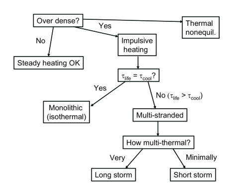
Figure 1.: Flow chart showing the logical progression used to infer the physical nature and heating of a coronal loop. Some boxes indicate observational questions and others indicate conclusions that are drawn from the answers.

2. Density

Suppose we wish to investigate an observed loop. We can start by asking the question “Is the loop over dense relative to static equilibrium?” Given the observed temperature and length, static equilibrium theory predicts a unique density. We want to know whether the observed density is larger than this value? If it is not, and if the loop does not evolve rapidly, then steady heating is a possible, though not unique, explanation. This was essentially where things stood through the Yohkoh mission in the 1990’s.

As we have already indicated, however, most EUV loops are indeed over dense. This is indicated in Figure 2 (reproduced from Klimchuk 2006), which reveals the physics of what is going on. The figure shows the ratio of the radiative to conductive cooling times plotted against temperature for a large sample of loops. The warm loops were observed by TRACE, and the hot loops were observed by Yohkoh/SXT. The ratio of the cooling times is determined from the measured temperature, density, and length according to $\tau_{rad}/\tau_{cond}=T^{4}/(n^{2}L^{2})$, although the power of temperature depends weakly on the radiative loss function and is slightly different in different temperature regimes.

Figure 2.: Ratio of radiative to conductive cooling times versus temperature for many observed loops. Solid line is the cooling track of an impulsively heated loop strand simulation. From Klimchuk (2006).

Coronal energy losses from radiation and thermal conduction are comparable for loops that are in static equilibrium (Vesecky, Antiochos, & Underwood 1979), and such loops would fall along a horizontal line near 0 in the plot. Loops that lie above the line are under dense, and loops that lie below the line are over dense. The observed loops follow a clear trend ranging from hot and under dense in the upper-right to warm and over dense in the lower-left. Note, however, that the densities used for the cooling time ratios were measured using emission measures and loop diameters and assuming a filling factor of unity, $n=[EM/(df)]^{1/2}$, so they are lower limits. Smaller filling factors would shift the points downward in the plot. Thus, the hot loops could be in static equilibrium, and the warm loops could be even more over dense than indicated.

It is abundantly clear that static equilibrium cannot explain warm loops. An explanation relying on steady end-to-end flows is also not viable (Patsourakos, Klimchuk, & MacNeice 2004). Thermal nonequilibrium is a possibility that we return to later. The most promising explanation for the observed over densities of warm loops is implusive heating. This can also explain the under densities of hot loops, if they are real. The solid curve that fits the points so well in Figure 2 is the evolutionary track from a 1D hydrodynamic simulation of a loop that has been heated impulsively by a nanoflare. Cooling begins at the upper-right end of the track and progresses downward and to the left. The early stages are dominated by thermal conduction and are characterized by under densities, while the late stages are dominated by radiation and are characterized by over densities. The ability of nanoflare models to reproduce the observed densities of loops is well established (Klimchuk 2002; Warren, Winebarger, & Hamilton 2002; Winebarger, Warren, & Mariska 2003; Cargill & Klimchuk 2004; Klimchuk 2006).

3. Lifetime

If a loop is heated impulsively, then we might expect it to exist for approximately a cooling time (combining the effects of conduction and radiation), as determined from the observed temperature, density, and length. This is the next question in the flowchart. If the lifetime and cooling time are similar, we can conclude that the loop is a monolithic structure that heats and cools as a homogeneous unit, with uniform temperature over the cross section. Observations show that this is not case, however. The vast majority of loops live longer than a cooling time and sometimes much longer (e.g., Winebarger, Warren, & Seaton 2003; López Fuentes, Klimchuk, & Mandrini 2007). If these loops contain cooling plasma, then they cannot be monolithic. Rather, they must be bundles of thin, unresolved strands that are heated impulsively at different times. Although each strand cools rapidly, the composite bundle appears to evolve slowly (e.g., Winebarger, Warren, & Mariska 2003). Multi-stranded bundles of this type can explain a number of observed properties of warm loops: over density, long lifetime, super-hydrostatic scale height, and flat temperature profile. They can also explain the observed under density of hot loops. Realizing this was a time of rejoicing in the modeling community! But….

4. Thermal Distribution

An important prediction of the multi-strand model is that loops should have multi-thermal cross-sections. Since the unresolved strands are heated at different times, they will be in different stages of cooling and out of phase with each other. A critical question became “Are loops multi-thermal?” An intense debate ensued and continues to this day. Some have answered with a resounding yes (the “Schmelz camp,” e.g., Schmelz & Martens 2006) and others have answered with a resounding no (the “Aschwanden camp,” e.g., Aschwanden & Nightingale 2005). As we now demonstrate, however, it is not especially useful to phrase the multi-thermal question in a way that requires a binary response.

Imagine that a loop bundle is heated by a “storm” of nanoflares that occur randomly over a finite window in time. It is easy to see that the range of strand temperatures that are present at any given moment depends on the duration of the storm. For a very short storm, all of strands will be heated at about the same time and will cool together. The instantaneous thermal distribution of the loop will be narrow. In contrast, a storm that lasts longer than a cooling time will produce a much wider thermal distribution. Some strands will have just been heated and will be very hot; others will have cooled to intermediate temperatures; and still others will have had time to cool to much lower temperatures. The flowchart in Figure 1 therefore asks the more meaningful question “How multi-thermal is the loop?” A broad thermal distribution implies a long-duration nanoflare storm, and a narrow distribution implies a short-duration storm. It now appears that the multi-thermal and isothermal camps may both be correct.

The duration of the nanoflare storm also determines the lifetime of the loop bundle, so the thermal width and lifetime will be closely related. Figure 3 shows results for simulated nanoflare storms lasting 500, 2500, and 5000 s, top to bottom. The left column has light curves (intensity versus time) as would be observed in the 195 channel of TRACE, with sensitivity peaking near 1 MK. The right column has emission measure distributions, EM($T$) = $T\times\!$DEM($T$) cm^-5, at the time of peak 195 intensity. Only the coronal part of the loop is included; the transition region footpoints are neglected. All three of the storms are comprised of identical nanoflares that have triangular heating profiles lasting 500 s. They were simulated with our “0D” hydro code EBTEL and are the same as example 4 in Klimchuk, Patsourakos, & Cargill (2008). In actuality, Figure 3 was produced with only one simulation. The light curves and EM distributions were constructed using sliding time windows that correspond to the storm durations.

Figure 3.: Simulated 195 light curves (left) and emission measure distributions (right) for nanoflare storms lasting 500, 2500, and 5000 s, top to bottom. The instantaneous EM distributions are from the times of peak 195 intensity (t = 3958, 4705, 5445 s for the three storms).

As expected, both the lifetime and thermal width increase as the storms get longer. The full widths at half maximum (FWHM) of the light curves are 1098, 2579, and 5008 sec for the 500, 2500, and 5000 s storms, respectively. The FWHM of the EM distributions are 0.13, 0.23, and 0.36 in $\log T$. The full widths at the 1% levels are 0.24, 0.62, and 1.14 in $\log T$.

It may seem surprising at first that the EM distributions do not all reach the same maximum temperature, since the nanoflares are the same in all three storms. This is not because individual strands are reheated multiple times in the longer storms; all strands are heated only once. Rather, it is because the distributions are from the time of peak 195 intensity. In the short duration storm, all of the strands have cooled appreciably by the time the peak intensity is reached. Had we chosen to plot the distribution at an earlier time, it would still been narrow, but it would be shifted to higher temperature.

Warren et al. (2008) have made Gaussian fits to EM distributions observed by Hinode/EIS. They find a typical central temperature of 1.4 MK and a typical Gaussian half width of 0.3 MK. This corresponds to a FWHM in $\log T$ of roughly 0.24, which by Figure 3 implies a 195 lifetime of roughly 2500 s. Although Warren et al. did not measure the lifetimes of their loops, this value is consistent with the small number of 195 lifetimes that have been reported for other cases (Winebarger & Warren 2005; Ugarte-Urra, Winebarger, & Warren 2006). To our knowledge, there does not exist a single published example where both the thermal width and lifetime have been measured for the same loop. Making such measurements should be a high priority. It is a crucial consistency check of the nanoflare concept. Density measurements should be made at the same time.

5. Very Hot and Very Faint Plasma

The nanoflare model makes two observational predictions in addition to the ones we have already discussed. First, it predicts that small amounts of very hot ($>5$ MK) plasma should be present. Figure 4 shows two examples of long (infinite) duration storms, one comprised of relatively weak nanoflares and the other comprised of nanoflares that are ten times stronger. The solid curve in each case is the EM distribution for the whole loop, while the dashed and dot-dashed curves are the contributions from the coronal section and footpoints, respectively. We see that the EM of the hottest plasma is 1.5-2 orders of magnitude smaller than that of the most prevalent plasma. The reason is two-fold. First, the initial cooling after the nanoflare has occurred is very rapid, so the hottest plasma persists for a relatively brief period. Second, the densities are low during this early phase, because chromospheric evaporation has only just begun to fill the loop strand with plasma.

Figure 4.: Emission measure distributions for long (infinite) duration nanoflare storms comprised of weak (left) and strong (right) nanoflares: coronal section (dashed), transition region footpoints (dot-dashed), and whole loop (solid).

As a consequence of the small emission measures, the intensities of hot spectral lines and channels are predicted to be very faint. The intensities may be reduced still further by ionization nonequilibrium effects (Bradshaw & Cargill 2006; Reale & Orlando 2008). Low levels of super-hot emission have nonetheless been detected recently by the CORONAS, RHESSI, and Hinode missions (Zhitnik et al. 2006; McTiernan 2009; Patsourakos & Klimchuk 2009; Ko et al. 2009). In particular, EM distributions inferred from multi-filter XRT observations of two active regions suggest that the distributions may have two distinct components (Schmelz et al. 2009; Reale et al. 2009). The implications are considerable, since this would rule out a simple power-law energy distribution for the responsible nanoflares. Detailed modeling is now underway.

6. Flows

High-speed upflows that reach or exceed 100 km s^-1 are predicted during the early evaporation phase of a nanoflare event. Depending on the geometry of the observations, these can produce highly blue-shifted emission. The emission will be very faint, however, for the reasons given above. A composite spectral line profile from a bundle of unresolved strands will be dominated by the weakly red-shifted emission produced during the much longer radiative cooling phase, when the plasma slowly drains and condenses back onto the chromosphere. Signatures of evaporation take the form of blue wing enhancements on this main component (Patsourakos & Klimchuk 2006). They can be very subtle, and they only appear in lines that are well tuned to the temperature of the evaporating plasma. Significantly hotter and cooler lines are not expected to show evidence of evaporation.

We have performed sit-and-stare observations with Hinode/EIS and find blue wing asymmetries in Fe XVII ($T\approx 5$ MK) similar to those predicted by our nanoflare models (Patsourakos & Klimchuk 2006). The measurements are very challenging, however, due to the faint nature of the line. Hara et al. (2008) also report blue-wing asymmetries that are suggestive of nanoflares.

7. Thermal Nonequilibrium

We have worked our way down the flowchart of Figure 1 and concluded that the observed properties of many loops can be explained by storms of nanoflares occurring within bundles of unresolved strands. There remains the possibility, indicated in the upper right, that many loops can also be explained by thermal nonequilibrium. We consider this possibility now.

Thermal nonequilibrium is a fascinating phenomenon in which dynamic behavior is produced by perfectly steady heating (Antiochos & Klimchuk 1991; Karpen et al. 2001; Mueller, Peter, & Hansteen 2004; Karpen, Antiochos, & Klimchuk 2006). No equilibrium exists if the steady heating is sufficiently highly concentrated near the loop footpoints. Instead, the loop goes through periodic convulsions as it searches for a nonexistent equilibrium. Cold, dense condensations form, slide down the loop leg, and later reform in a cycle that repeats with periods of several tens of minutes to several hours.

We have recently explored whether thermal nonequilibrium can explain the observed properties of EUV loops (Klimchuk & Karpen 2009). We first considered a monolithic loop, which we simulated with our 1D hydro code ARGOS (Antiochos et al. 1999). The code uses adaptive mesh refinement, which is critical for resolving the thin transition regions that exist on either side of the dynamic condensations. We imposed a steady heating that decreases exponentially with distance from both footpoints. The heating scale length of 5 Mm is one-fifteenth of loop halflength. We introduced a small asymmetry by making the amplitude of the heating on the right side only 75% that on the left.

Figure 5 shows the evolution of temperature, density, and intensity as would be observed in the 171 channel of TRACE. These are averages over the upper 80% of the loop. The behavior is typical of the several cycles that we simulated. The loop is visible in 171 for only about 1000 s. This is a factor of 2-4 shorter than observed lifetimes (Winebarger & Warren 2005; Ugarte-Urra, Winebarger, & Warren 2006). A more serious problem is the distribution of emission along the loop (the intensity profile), which disagrees dramatically with observations. Figure 6 shows 171 intensity and temperature as a function of position along the loop at $t=5000$ s. The emission is strongly concentrated in transition region layers at the loop footpoints ($s=45$ and $203$ Mm) and to either side of a cold condensation at $s=163$ Mm. In stark contrast, most observed 171 loops have a fairly uniform brightness along their length.

Figure 5.: Evolution of temperature (dashed), density (dotted), and 171 intensity (solid) for a monolithic loop undergoing thermal nonequilibrium. All quantities are normalized. The steady heating is 75% as strong in the right leg as in the left.

Figure 6.: Temperature (dashed, MK) and 171 intensity (solid, arbitrary units) as a function of position along the loop at $t=5000$ s in the simulation of Figure 5.

The maximum temperature in the loop is 4.4 MK and occurs before the condensation forms. We performed another simulation with a reduced heating rate that has a maximum temperature of only 1.8 MK. Neither the light curve nor the intensity profile are consistent with observations. We conclude that EUV loops are not monolithic structures undergoing thermal nonequilibrium, at least not under conditions that lead to cold condensations. We note, however, that Mok et al. (2008) report a different type of nonequilibrium behavior. One prominent loop in their 3D simulation of an active region exhibits a cooling and heating cycle, but the temperature never drops to the point where a condensation forms. The reasons for the differing behavior are yet to be understood. Whether the loop has properties matching observed loops (density, lifetime, thermal width) is unknown.

The simulation of Figures 5 and 6 may nonetheless have some relevance to the Sun. The condensation falls onto the right footpoint at $t=5600$ s. Falling condensations have been seen in the C IV channel of TRACE (Schrijver 2001). They are relatively rare, however, and occur in only a small fraction of loops.

We next considered the possibility of a multi-stranded loop bundle in which the individual strands undergo thermal nonequilibrium in an out-of-phase fashion. To approximate such a loop, we performed two additional simulations, similar to the first but with heating imbalances of 50% and 90% instead of 75%. We then averaged all three simulations in time and added them together along with their mirror images to form a composite loop. The resulting 171 intensity profile is shown in Figure 7. It is reasonably uniform except for the very intense spikes at the footpoints (note the logarithmic scale). A more realistic loop bundle with a wider variety of heating imbalances would be even more uniform. We tentatively conclude that the intensity profile is consistent with observations, although we are concerned because bright 171 moss emission is generally observed at the footpoints of SXR loops rather than the footpoints of EUV loops.

Figure 7.: Logarithm of 171 intensity as a function of position along a composite loop bundle comprised of individual strands undergoing thermal nonequilibrium. See text for details.

Figure 8.: Temperature as a function of position along the composite loop bundle of Figure 7. Solid is the actual mean temperature, while dashed and dotted are the temperatures inferred from TRACE and Yohkoh/SXT filter ratios, respectively.

Figure 8 shows three temperature profiles for the composite loop: the average of the actual temperatures in the individual strands (solid), the temperature that would be inferred from TRACE 171/195 intensity ratios (dashed), and the temperature that would be inferred from Yohkoh/SXT Al12/AlMg intensity ratios (dotted). They are different because Yohkoh/SXT is more sensitive to the hotter plasma and TRACE is more sensitive to the warmer plasma. Notice that the profiles is very flat. This is a well-know property of EUV loops. We have also inferred densities from the simulated TRACE observations using exactly the same procedure that was used for the real loops in Figure 2. The model loop is over dense by a factor of 23, consistent with observed values. We have repeated this excise using reduced heating in the strands and find that the over density is a factor of 10 in this case.

Although there is some reason for encouragement, it is not obvious that bundles of unresolved strands undergoing thermal nonequilibrium can explain all the salient properties of observed EUV loops. Reproducing the lifetimes is especially challenging. The condensations in the different strands must be sufficiently out of phase to give a uniform intensity profile, but they cannot be so out of phase as to produce a composite loop lifetime longer than 1 hour. Even if the phasing is correct for one condensation cycle, it is likely to be incorrect for subsequent cycles because the interval between condensations depends on both the amplitude of the heating and its left-right imbalance. The imbalance determines the location where the condensation forms, and it must be appreciably different among the strands in order to get a uniform intensity profile. Note that the results shown in Figures 7 and 8 make use of temporal averages over complete cycles, and therefore the lifetime of the equivalent loop bundle is effectively infinite.

8. Conclusions

We have described how a combination of observational and modeling work has led to the conclusion that warm ($\sim 1$ MK) EUV loops can be explained as bundles of unresolved strands that are heated by storms of nanoflares. Static equilibrium is out of the question. The observed lifetimes and thermal distributions of the plasma indicate that the storms last for typically 2-4$\times 10^{3}$ s. Additional support for this picture is provided by the shapes of hot spectral line profiles and by the observation that line intensities peak at slightly later times for lines of progressively cooler temperature (Ugarte-Urra, Warren, & Brooks 2009). Also, there is now good evidence for very hot and very faint plasma, as predicted by the nanoflare models.

It is not clear whether most hot ($>2$ MK) SXR loops are also heated by nanoflares. If they are, the storms must be long duration in order to explain the observed lifetimes. The loops would then be expected to have co-spatial EUV counterparts, and it is not obvious that they do. One possibility is that the frequency of nanoflares is much higher in long-lived SXR loops, so that the plasma in a strand never cools to EUV temperatures before being reheated. It is worth noting that virtually all of the proposed coronal heating mechanisms predict impulsive energy release on individual magnetic field lines (Klimchuk 2006).

We considered the possibility that EUV loops can be explained by thermal nonequilibrium. We concluded that this is not a viable mechanism for monolithic loops under the conditions we have considered—although the results of Mok et al. (2008) are very intriguing—but that it may have application in multi-stranded bundles. Serious questions remain that require further investigation.

We close by pointing out that distinct loops are only one component of the corona and that the diffuse component contributes at least as much emission. It is not generally appreciated that the intensity of EUV and SXR loops is typically much less than that of the background (of order 10-40%). The diffuse component may also be made up of individual strands, but we must explain why the strands have a higher concentration in loops.

Acknowledgments.

I am very pleased to acknowledge useful discussions with many people, but I especially wish to thank Spiros Patsourakos, Harry Warren, and Judy Karpen, my collaborator on the thermal nonequilibrium study that is being published here for the first time. I benefited greatly from participation in the Coronal Loops Workshop Series and the International Space Science Institute team led by Susanna Parenti. Financial support came primarily from the NASA Living With a Star program.

References

- Antiochos & Klimchuk (1991) Antiochos, S. K., & Klimchuk, J. A. 1991, ApJ, 378, 372
- Antiochos et al. (1999) Antiochos, S. K., MacNeice, P. J., Spicer, D. S.,& Klimchuk, J. A. 1999, ApJ, 512, 985
- Aschwanden & Nightingale (2005) Aschwanden, M. J., & Nightingale, R. W. 2005, ApJ, 633, 499
- Aschwanden, Schrijver, & Alexander (2001) Aschwanden, M. J., Schrijver, C. J., & Alexander, D. 2001, ApJ, 550, 1036
- Aschwanden et al. (1999) Aschwanden, M. J., Newmark, J. S., Delaboudiniere, J. P., Neupert, W. M., Klimchuk, J. A., Gary, G. A., Portier-Fornazzi, F., & Zucker, A. 1999, ApJ, 515, 842
- Bradshaw & Cargill (2006) Bradshaw, S. J. & Cargill, P. J. 2006, A&A, 458, 987
- Cargill & Klimchuk (2004) Cargill, P. J. & Klimchuk, J. A. 2004, ApJ, 605, 911
- Hara et al. (2008) Hara, H. et al. 2008, ApJ(Lett), 678, L67
- Kano & Tsuneta (1996) Kano, R., & Tsuneta, S. 1996, PASJ, 48, 535
- Karpen et al. (2001) Karpen, J. T., Antiochos, S. K., Hohensee, M., Klimchuk, J. A., & MacNeice, P. J. 2001, ApJ(Lett), 553, L85
- Karpen, Antiochos, & Klimchuk (2006) Karpen, J. T., Antiochos, S. K., & Klimchuk, J. A. 2006, ApJ, 637, 531
- Klimchuk (2002) Klimchuk, J. A. 2002, in ITP Conf. on Solar Magnetism and Related Astrophysics, U. California Santa Barbara, ed. G. Fisher and D. Longcope (http://online.kitp.ucsb.edu/online/solar_c02/klimchuk/).
- Klimchuk (2006) Klimchuk, J. A. 2006, Solar Phys., 234, 41
- Klimchuk & Karpen (2009) Klimchuk, J. A., & Karpen, J. T. 2009, in preparation
- Klimchuk, Patsourakos, & Cargill (2008) Klimchuk, J. A., Patsourakos, S., & Cargill, P. J. 2008, ApJ, 682, 1351
- Ko et al. (2009) Ko, Y.-K. et al. 2009, ApJ, submitted
- Lenz et al. (1999) Lenz, D. D., DeLuca, E. E., Golub, L., Rosner, R., & Bookbinder, J. A. 1999, ApJ, 517, L15
- López Fuentes, Klimchuk, & Mandrini (2007) López Fuentes, M. C., Klimchuk, J. A., & Mandrini, C. H. 2007, ApJ, 657, 1127
- McTiernan (2009) McTiernan, J. M. 2009, ApJ, submitted
- Mok et al. (2008) Mok, Y., Mikić, Z., Lionello, R., & Linker, J. A. 2008, ApJ(Lett), 679, L161
- Mueller, Peter, & Hansteen (2004) Mueller, D. A. N., Peter, H., & Hansteen, V. H. 2004, A&A, 424, 289
- Patsourakos, Klimchuk, & MacNeice (2004) Patsourakos, S., Klimchuk, J. A., & MacNeice, P. J. 2004, ApJ, 603, 322
- Patsourakos & Klimchuk (2006) Patsourakos, S., & Klimchuk, J. A. 2006, ApJ, 647, 1452
- Patsourakos & Klimchuk (2009) Patsourakos, S., & Klimchuk, J. A. 2009, ApJ, in press
- Porter & Klimchuk (1995) Porter, L. J., & Klimchuk, J. A. 1995, ApJ, 454, 499
- Reale & Orlando (2008) Reale, F. & Orlando, S. 2008, ApJ, 284, 715
- Reale et al. (2009) Reale, F., Testa, P., Klimchuk, J. A., & Parenti, S. 2009, ApJ, submitted
- Rosner, Tucker, & Vaiana (1978) Rosner, R., Tucker, W. H., & Vaiana, G. S. 1978, ApJ, 220, 643
- Schmelz & Martens (2006) Schmelz, J. T., & Martens, P. C. H. 2006, ApJ(Lett), 636, L49
- Schmelz et al. (2009) Schmelz, J. T. et al. 2009, ApJ(Lett), in press
- Schrijver (2001) Schriver, C. J. 2001, Solar Phys., 198, 325
- Ugarte-Urra, Warren, & Brooks (2009) Ugarte-Urra, I., Warren, H. P., & Brooks, D. H. 2009, ApJ, in press
- Ugarte-Urra, Winebarger, & Warren (2006) Ugarte-Urra, I., Winebarger, A. R., & Warren, H. P. 2006, ApJ, 643, 1245
- Vesecky, Antiochos, & Underwood (1979) Vesecky, J. F., Antiochos, S. K., & Underwood, J. H. 1979, ApJ, 233, 987
- Warren et al. (2008) Warren, H. P., Ugarte-Urra, I., Doschek, G. A., Brooks, D. H., & Williams, D. R. 2008, ApJ(Lett), 686, L131
- Warren, Winebarger, & Hamilton (2002) Warren, H. P., Winebarger, A. R., & Hamilton, P. S. 2002, ApJ (Lett), 579, L41
- Warren, Winebarger, & Mariska (2003) Warren, H. P., Winebarger, A. R., & Mariska, J. T. 2003, ApJ, 593, 1174
- Winebarger & Warren (2005) Winebarger, A. R., & Warren, H. P. 2005, ApJ, 626, 543
- Winebarger, Warren, & Mariska (2003) Winebarger, A. R., Warren, H. P., & Mariska, J. T. 2003, ApJ, 587, 439
- Winebarger, Warren, & Seaton (2003) Winebarger, A. R., Warren, H. P., & Seaton, D. B. 2003, ApJ, 593, 1164
- Zhitnik et al. (2006) Zhitnik, I. A. et al. 2006, Solar System Research, 40, 272