Correlated Gaussian Hyperspherical Method for Few-Body Systems

Abstract

We develop an innovative numerical technique to describe few-body systems. Correlated Gaussian basis functions are used to expand the channel functions in the hyperspherical representation. The method is proven to be robust and efficient compared to other numerical techniques. The method is applied to few-body systems with short range interactions, including several examples for three- and four-body systems. Specifically, for the two-component, four-fermion system, we extract the coefficients that characterize its behavior at unitarity.

I Introduction

Ultracold gases in traps or optical lattices have opened new possibilities in the study of strongly correlated quantum systems. From the rich few-body physics of the Efimov effect braaten2006ufb ; efim70 ; esry1999rta ; kraemer2006eeq to the fascinating many-body physics of the BCS-BEC crossover eagl69 ; legg80 ; nozieres1985bca ; greiner2003emb ; jochim2003bec ; zwierlein2003obe ; bour04 ; regal2004orc ; zwierlein2004cpf ; zwierlein2005vas , experimentalists are now able to realize a wide variety of physical systems of great interest for the atomic, nuclear, and condensed matter communities. In particular, the pureness and controllability of cold atoms in optical lattices jaksch1998cba ; paredes2004fa ; kinoshita2004ood make them perfect candidates for the experimental implementation of condensed matter models [see Ref. bloch2008mbp and references therein]. In all these systems, the rich physics that governs a few interacting atoms is crucial for understanding recent experiments.

For that reason, extensive efforts have concentrated on the development of an accurate description of few-body systems. Encouraging advances have been achieved in the last decade in the understanding ultracold three-body problem braaten2006ufb ; esry1999rta ; PhysRevLett.93.143201 ; PhysRevA.67.010703 . These studies have demonstrated the importance of three-body recombination and relaxation processes and have determined the effective interaction in atom-dimer collisions. Some of these techniques were subsequently extended to four-body systems  petrov2004wbd ; deltuva2007fbc ; stech07 ; dincao08 ; wang2008etf , in a few applications. However, the physics of the four-body problem that are far richer and more complicated. Also, it is a very challenging numerical problem and for that reason it has remained largely unsolved except in very limited regimes. Here, we present a novel numerical method to handle few-body systems that can be used to efficiently describe four-body systems, through a combination of different techniques.

Even though several techniques have been developed in recent decades to provide solutions for few-body systems  faddeev1960mat ; suzuki1998sva ; malfliet1969sfe ; yaku67 ; mace68 , not many of them have been applied to numerically solve the Schrödinger equation for systems with more than three particles. Among these methods, the correlated Gaussian (CG) technique singer1960uge ; boys1960ifv ; kukulin1977svm ; varga1996svm ; varga1995psf ; varga1997sfb ; varga1994mmd in particular has proven to be capable of describing a trapped few-body system with short-range interactions. Because of the simplicity of the matrix element calculation, the CG method provides an accurate description of the ground and excited states up to $N=6$ particles varga1995psf ; varga1997sfb ; blumePRL07 . However, the CG method as previously implemented can only describe bound states. For this reason, previous studies have focused on trapped systems where all the eigenstates are discrete vonstech07 ; vonstech08a ; stech07 ; blumePRL07 . In fact, the CG method requires a nontrivial extension in order to describe the continuum and the rich behavior of atomic collisions, such as dissociation, rearrangement, and recombination processes.

The hyperspherical representation, in fact, provides an appropriate framework that can treat the continuum Delves59 ; Delves60 ; mace68 ; Lin95 ; Shitikova77 ; Chapuisat92 . In the adiabatic hyperspherical representation, the Hamiltonian is diagonalized as a function of the hyperradius $R$, reducing the Schrödinger equation to a set of coupled equations in a single variable, with a series of different effective potentials and couplings. The asymptotic behavior of the channel potentials describes different dissociation or fragmentation pathways and provides a suitable framework for analyzing collision physics. These solutions can be readily combined with scattering methods such as the R-matrix approach aymar1996mrs ; zatsarinny2004bsb ; sunderland2002prm to provide an accurate description of the collisional dynamics. However, the standard hyperspherical methods expand the hyperangular channel functions in a B-spline or finite element basis set pack1987qrs ; zhou1993hac ; esry1996ahs ; suno2002tbr , and the calculations become very computationally demanding for $N>3$ systems.

It is therefore natural to combine the scalability of the CG method with the advantages of the hyperspherical representation. In this article, we present an innovative way to achieve this combination, in what we term the correlated Gaussian hyperspherical method (CGHS). This method uses CG basis functions to expand the channel functions in the hyperspherical representation. We show that also in this case, the matrix element evaluation is greatly simplified thanks to the simple form of the CG basis functions. Furthermore, thanks to the explicit correlation incorporated in these basis functions, only a relatively small basis set is needed to achieve convergence of the lowest channel functions even in the strongly interacting regime.

To illustrate the power of the CGHS method, we carry out calculations for $N=3,4$-particle systems in the strongly interacting regime. First, we analyze systems of three-bosons or three fermions at unitarity, and show that the method recovers results that agree with semi-analytical predictions. Then, we consider the two-component four-fermion system, in the large and positive scattering length regime, and reproduce the lowest potential curves from Ref. dincao08 . The CGHS provides a larger number of channels which would allow the calculation of scattering events not considered in Ref. dincao08 . Finally, we focus on the universal behavior of four-fermions at unitarity. In this regime, the energies of the trapped system are trivially determined by the hyperspherical potential curves wern06 ; blumePRL07 . Therefore, we can compare our calculations with predictions for the trapped system stech07 ; chan07 ; vonstechtbp ; alhassid08 ; StetcuCM07 . Our results improve and extend these previous predictions, and characterize the 20 lowest potential curves for even parity and vanishing orbital angular momentum.

This article continues as follows. First, we review both the CG and hyperspherical methods in Sec. II. In Sec. III, we introduce the main idea of the CGHS method, leaving some details of the implementation for the Appendix A. Sec. IV presents our results for three-body systems and for the four-fermion system. Finally, Sec. V presents our conclusions.

II Theoretical background

This section discusses the general problem to be solved and reviews the correlated Gaussian method. Subsec. II.2 presents the general formalism of the hyperspherical representation and describes how to numerically solve the Schrödinger equation in this representation using a correlated Gaussian basis set expansion.

The methods described in this article solve the time-independent Schrödinger equation for a Hamiltonian of the form

$$H=\sum_{i}\left(\frac{-\hbar^{2}}{2m_{i}}\nabla_{i}^{2}+V_{ext}(\mathbf{r}_{i})\right)+\sum_{i,j}V_{0}(r_{ij}).$$ (1)

where $V_{ext}$ is an external trapping potential and $V_{0}$ is the interaction potential. The form of the Hamiltonian can be varied depending on the particular problem we are considering. In the CG method one will usually consider a spherically-symmetric harmonic trapping potential $V_{ext}(\mathbf{r})=\frac{1}{2}m_{i}\omega^{2}\mathbf{r}_{i}^{2}$ but in hyperspherical calculations we usually consider a free system ($V_{ext}(\mathbf{r})=0$). We can always include the harmonic trapping potential in the final step of the hyperspherical calculation, since it is a purely hyperradial potential. Depending on the particular problem considered, the interacting particles will change. For example, all particles interact with each other in identical boson systems but only opposite-spin fermions interact in two-component Fermi systems (except in a few problems involving $p$-wave Fano-Feshbach resonances). Also, in many cases, the center-of-mass motion decouples from the more interesting internal degrees of freedom, and it is preferable to use a set of Jacobi coordinates rather than the usual single-particle coordinates. All such options can be treated using the method presented below.

II.1 Correlated Gaussian Method

Different types of Gaussian basis functions have long been used in many different areas of physics. In particular, the usage of Gaussian basis functions is one of the key elements of the success of ab initio calculations in quantum chemistry. The idea of using an explicitly correlated Gaussian to solve quantum chemistry problems was introduced in 1960 by Boys boys1960ifv and Singer singer1960uge . The combination of a Gaussian basis and the stochastical variational method (SVM) was first introduced by Kukulin and Krasnopol’sky kukulin1977svm in nuclear physics and was extensively used by Suzuki and Varga varga1996svm ; varga1995psf ; varga1997sfb ; varga1994mmd . These methods were also used to treat ultracold many-body Bose systems by Sorensen, Fedorov and Jensen sorensen2005cgm . A detailed discussion of both the SVM and CG methods can be found in a thesis of Sorensen sorensen2005cmb and, in particular, in the book by Suzuki and Varga suzuki1998sva . In the following, we highlight the main ideas of the CG method.

Consider a set of coordinate vectors that describe the system $\{\mathbf{x}_{1},...,\mathbf{x}_{N}\}$. In this method, the eigenstates are expanded in a set of basis functions,

$$\Psi(\mathbf{x}_{1},\cdots,\mathbf{x}_{N})=\sum_{A}C_{A}\,\Phi_{A}(\mathbf{x}_{1},\cdots,\mathbf{x}_{N}).$$ (2)

Here $A$ specifies a matrix with a particular set of parameters that characterize the basis function. It is convenient to introduce the following ket notation, $\Phi_{A}(\mathbf{x}_{1},\cdots,\mathbf{x}_{N})=\mathinner{\langle{\mathbf{x}_{1},\cdots,\mathbf{x}_{N}|A}\rangle}$. Solution of the time-independent Schrödinger equation in this basis set reduces the problem to one of diagonalizing the Hamiltonian matrix:

$$\mathcal{H}\vec{C}_{i}=E_{i}\mathcal{O}\vec{C}_{i}$$ (3)

Here, $E_{i}$ are the energies of the eigenstates, $\vec{C}_{i}$ is a vector formed with the coefficients $C_{A}$ and $\mathcal{H}$ and $\mathcal{O}$ are matrices whose elements are $\mathcal{H}_{BA}=\mathinner{\langle{B|\mathcal{H}|A}\rangle}$ and $\mathcal{O}_{BA}=\mathinner{\langle{B|A}\rangle}$. For a 3D system, the evaluation of these matrix elements involves $3N$-dimensional integrations which are in general very expensive to compute. Therefore, the effectiveness of the basis set expansion method relies mainly on the appropriate selection of the basis functions. As we will see, the CG basis functions permit fast evaluation of overlap and Hamiltonian matrix elements, and they are flexible enough to correctly describe physical states.

To reduce the dimensionality of the problem we can take advantage of its symmetry properties. Since the interactions considered are spherically symmetric, the total angular momentum, $L$, is a good quantum number. For simplicity, we will restrict ourselves to $L=0$ solutions. This restriction allows us to reduce the Hilbert space by introducing restrictions on the basis functions. In particular, if the basis functions only depend on the interparticle distances, then Eq. (2) can only describe states with zero angular momentum and positive parity ($L^{P}=0^{+}$). Furthermore, we can recognize that the center-of-mass motion decouples from the system. In such cases, the CG basis functions take the form

$$\Phi_{A}(\mathbf{x}_{1},\cdots,\mathbf{x}_{N})=\psi_{0}(\mathbf{R}_{CM})\mathcal{S}\left\{\exp\left(-\sum_{j>i=1}^{N}\alpha_{ij}r_{ij}^{2}/2\right)\right\},$$ (4)

where $\mathcal{S}$ is a symmetrization operator and $r_{ij}$ is the interparticle distance between particles $i$ and $j$. Here, $\psi_{0}$ is the ground state of the center-of-mass motion. For trapped systems, $\psi_{0}$ takes the form, $\psi_{0}(\mathbf{R}_{CM})=e^{-R_{CM}^{2}/2(a_{ho}^{M})^{2}}$. Because of its simple Gaussian form, $\psi_{0}$ can be absorbed in the exponential factor. Thus, in a more general way, the basis function can be written in terms of a matrix $A$ that characterizes them,

$$\Phi_{A}(\mathbf{x}_{1},\mathbf{x}_{2},...,\mathbf{x}_{N})=\mathcal{S}\left\{\exp(-\frac{1}{2}\mathbf{x}^{T}.A.\mathbf{x})\right\}\\ =\mathcal{S}\left\{\exp(-\frac{1}{2}\sum_{j,i=1}^{N}A_{ij}\mathbf{x}_{i}.\mathbf{x}_{j})\right\},$$ (5)

where $\mathbf{x}=\{\mathbf{x}_{1},\mathbf{x}_{2},...,\mathbf{x}_{N}\}$, and $A$ is a symmetric matrix. The matrix elements $A_{ij}=A_{ji}$ can be expressed in terms of the $\alpha_{ij}$. Because of the simplicity of the basis functions, Eq. (4), the matrix elements of the Hamiltonian can be calculated analytically.

The analytical evaluation of the matrix elements is enabled by selecting the set of coordinates that simplifies the evaluations. For basis functions of the form of Eq. (5), the matrix elements are characterized by a matrix $M$ in the exponential. Then the matrix element integrand greatly simplifies if we rewrite it in terms of the coordinate vectors that diagonalize that matrix $M$. This change of coordinates permits, in many cases, the analytical evaluation of the matrix elements. The explicit evaluation of several matrix elements can be found in Refs. sorensen2005cmb ; suzuki1998sva .

Two properties of the CG method deserve mention at this point. First, the CG method does not rely on any approximation other than basis set truncation, and the solutions can be systematically improved. The accuracy of the results are only limited by numerical issues related to linear dependence of the basis set. Secondly, the basis functions $\Phi_{A}$ are square-integrable only if the matrix $A$ is positive definite. This ensures that the wave function decays in all degrees of freedom. We can further restrict the basis functions by introducing real widths $d_{ij}$ such that $\alpha_{ij}=1/d_{ij}^{2}$. With this transformation, we ensure that $A$ is positive definite. Furthermore, each such width is proportional to the mean interparticle distances covered by that basis function. Thus, it is relatively easy to select the widths after considering the physical length scales relevant to the problem. Even though we have restricted the Hilbert space with this transformation, we have numerical evidence that the results converge to the exact eigenvalues.

The linear dependence in the basis set causes problems in the numerical diagonalization of the Hamiltonian matrix, Eq. (3). To minimize these linear dependence problems we restrict the basis function so that the overlap between any two normalized basis functions is below some cutoff value. The other method we use to eliminate linear dependence applies a linear transformation to produce a smaller orthonormal basis set.

Finally, we stress the importance of making an appropriate selection of the interaction potential. For the problems considered in this article, the interactions are expected to be characterized only by the scattering length, i.e., to be independent of the shape of the potential. For that reason, we can select a model potential that permits rapid evaluation of the matrix elements. We have found that a model potential with a Gaussian form,

$$V_{0}(r)=-V_{0}\exp\left(-\frac{r^{2}}{2r_{0}^{2}}\right),$$ (6)

is particularly suitable for this basis set expansion since it can be absorbed in the exponential form of the wave functions for matrix element evaluation. If the range $r_{0}$ is much smaller than the scattering length, then the interactions are effectively characterized only by the scattering length. The scattering length is tuned by changing the strength of the interaction potential, $V_{0}$, while the range, $r_{0}$, of the interaction potential remains unchanged. This is particularly convenient in this method since it implies that we only need to evaluate the matrix elements once and we can use them to solve the Schrödinger equation at any given potential strength (or scattering length). Of course, this procedure will give accurate results only if the basis set is sufficiently flexible and complete to describe the different configurations that appear at different scattering lengths.

In general, this method includes five basic steps: generation of the basis set, evaluation of the matrix elements, elimination of linear dependence, evaluation of the eigenvalue spectrum, followed by a study of stability and convergence. The stochastic variational method (SVM) Refs. sorensen2005cmb ; suzuki1998sva combines the first three of these steps in an optimization procedure where the basis functions are selected randomly.

II.2 Hyperspherical representation

The main objective of the hyperspherical method is to solve the time-independent Schrödinger equation in a convenient and efficient way that also provides insight into the relevant reaction pathways by which various collision processes can occur. the first step involves calculation of eigenvalues and eigenfunctions of the fixed-hyperradius Hamiltonian, which defines the adiabatic hyperspherical representation. These eigenvalues and eigenfunctions are then used to construct a set of one-dimensional coupled equations in the hyperradius $R$. The hyperradius is a collective coordinate related to the total moment of inertia of the systemShitikova77 ; fano1981 . In a system described by $N$ coordinate vectors $\mathbf{r}_{1},\ldots,\mathbf{r}_{N}$, the hyperradius $R$ is defined by

$$\mu R^{2}=\sum_{i=1}^{N}m_{i}\mathbf{r}_{i}^{2}.$$ (7)

Here, $\mu$ is an arbitrary mass factor called the hyperradial reduced mass fnote1 and $m_{i}$ are the masses corresponding to the particle $i$. The remaining coordinates are described by a set of hyperangles, collectively denoted $\Omega$.

The total number of spatial dimensions of this $N$-particle system is $d=3\,N$. The total wave function $\psi$ is rescaled by $R$, $\Psi=R^{(d-1)/2}\psi$, so that the hyperradial equation resembles a coupled one-dimensional Schrodinger equation. In the adiabatic representation, the wave function $\Psi_{E}(R,\Omega)$ is expanded in terms of a complete orthonormal set of angular wave functions $\Phi_{\nu}$ and radial wave functions $F_{\nu E}$, such that

$$\Psi_{E}(R,\Omega)=\sum_{\nu}F_{\nu E}(R)\Phi_{\nu}(R;\Omega).$$ (8)

The adiabatic eigenfunctions, or channel functions $\Phi_{\nu}$, depend parametrically on $R$ and are eigenfunctions of a $3\,N-1$ partial differential equation (which reduces to $3N-4$ dimensions if the center-of-mass motion is removed explicitly):

$$\left(\frac{\hbar^{2}\Lambda^{2}}{2\mu R^{2}}+\frac{(d-1)(d-3)\hbar^{2}}{8\mu R^{2}}+V(R,\Omega)\right)\Phi_{\nu}(R;\Omega)\\ =U_{\nu}(R)\Phi_{\nu}(R;\Omega).$$ (9)

Here, $\Lambda$ is the grand angular momentum operator, which is related to the kinetic term by

$$-\sum_{i}\frac{\hbar^{2}\nabla_{i}^{2}}{2m_{i}}=-\frac{\hbar^{2}}{2\mu}\frac{1}{R^{d-1}}\frac{\partial}{\partial R}R^{d-1}\frac{\partial}{\partial R}+\frac{\Lambda^{2}\hbar^{2}}{2\mu R^{2}}.$$ (10)

The $U_{\nu}(R)$ obtained in Eq. (9) are effective hyperradial potential curves that appear in a set of coupled one-dimensional differential equations:

$$\left[-\frac{\hbar^{2}}{2\mu}\frac{d^{2}}{dR^{2}}+U_{\nu}(R)\right]F_{\nu E}(R)\\ -\frac{\hbar^{2}}{2\mu}\sum_{\nu^{\prime}}\left[2P_{\nu\nu^{\prime}}(R)\frac{d}{dR}+Q_{\nu\nu^{\prime}}(R)\right]F_{\nu^{\prime}E}(R)=EF_{\nu E}(R).$$ (11)

These differential equations [Eq. (11)] are coupled through the $P_{\nu\nu^{\prime}}(R)$ and $Q_{\nu\nu^{\prime}}(R)$ couplings defined as

$$P_{\nu\nu^{\prime}}(R)=\mathinner{\langle{\Phi_{\nu}(R;\Omega)|\frac{\partial}{\partial R}|\Phi_{\nu^{\prime}}(R;\Omega)}\rangle}\Big{|}_{R},$$ (12)

$$Q_{\nu\nu^{\prime}}(R)=\mathinner{\langle{\Phi_{\nu}(R;\Omega)|\frac{\partial^{2}}{\partial R^{2}}|\Phi_{\nu^{\prime}}(R;\Omega)}\rangle}\Big{|}_{R}.$$ (13)

Since the basis set expansion of the wave function, Eq. (8), is complete in the $3\,N$-dimensional space, Eqs. (9) and (11) reproduce exactly the original $d$-dimensional Schrödinger equation. As in most numerical methods, the solutions are approximated by truncating the Hilbert space. In this case, the Hilbert space is truncated by considering a finite number of channels in Eq. (11). This approximation is easily tested by analyzing convergence with respect to the number of channels included in the calculation.

The utility of the hyperspherical representation relies on the assumption that the wavefunction variation with the hyperradius $R$ is smooth. In such cases, only a few channels are relevant, and the couplings are small and vary smoothly with $R$. Furthermore, a fairly good approximation to the solutions can be achieved by truncating the expansion in Eq. (8) to a single term:

$$\Psi_{E}(R,\Omega)=F_{\nu E}(R)\Phi_{\nu}(R;\Omega).$$ (14)

This adiabatic hyperspherical approximation leads to an effective one-dimensional Schrödinger equation,

$$\left[-\frac{\hbar^{2}}{2\mu}\frac{d^{2}}{dR^{2}}+W_{\nu}(R)\right]F_{\nu E}(R)=EF_{\nu E}(R),$$ (15)

where the effective potential is

$$W_{\nu}(R)=U_{\nu}(R)-\frac{\hbar^{2}}{2\mu}Q_{\nu\nu}(R).$$ (16)

Here, the first term is the hyperradial potential curve, and the second term is “adiabatic correction”, i.e. the repulsive kinetic contribution of the hyperradial dependence of the channel function. If the potential curves are well-separated and have no strong avoided crossings in the relevant range of energy and radius, then the adiabatic approximation can be quite accurate for the lower states in any given potential curve. This approximation comes from a truncation of the Hilbert space and, for that reason, obeys the variational principle. Any discrete energy eigenvalue obtained with this method is an upper bound of the exact energy level, in the sense of the Hylleraas-Undheim theorem. An approximate description of the spectrum can be achieved by combining the energies obtained from the adiabatic approximation applied to each channel separately. For example, bound states of excited potential curves which are above the lowest fragmentation threshold would represent quasi-bound states. This approach is equivalent to neglecting all off-diagonal couplings in Eq. (11) and produces an approximate spectrum which is not variational. Another useful approximation is obtained by neglecting the second term in Eq. (16), i.e., replacing $W_{0}(R)$ by $U_{0}(R)$ in Eq. (15). This is usually called the hyperspherical Born-Oppenheimer approximation. As in the standard Born-Oppenheimer approximation for a diatomic molecule, the approximate energy obtained in this manner represents a lower bound to the exact ground state energy Coelho91 .

Next, we show how Eq. (9) is solved, and how the $P_{\nu\nu^{\prime}}$ and $Q_{\nu\nu^{\prime}}$ are evaluated.

II.3 Expansion of the channel function in a basis set

In the hyperspherical method (see Sec. II.2), channel functions are eigenfunctions of the adiabatic Hamiltonian $\mathcal{H}_{A}(R;\Omega)$,

$$\mathcal{H}_{A}(R;\Omega)\Phi_{\nu}(R;\Omega)=U_{\nu}(R)\Phi_{\nu}(R;\Omega).$$ (17)

The eigenvalues of this equation are the hyperspherical potential curves $U_{\nu}(R)$, which serve as readily visualizable reaction pathways. The adiabatic Hamiltonian has the form:

$$\mathcal{H}_{A}(R;\Omega)=\frac{\hbar^{2}\Lambda^{2}}{2\mu R^{2}}+\frac{(d-1)(d-3)\hbar^{2}}{8\mu R^{2}}+V(R,\Omega).$$ (18)

Here, $d=3N_{J}$ where $N_{J}$ is the number of Jacobi coordinate vectors.

A standard way to solve Eq. (17) is to expand the channel functions in a basis,

$$\mathinner{|{\Phi_{\mu}(R;\Omega)}\rangle}=\sum_{i}\mathinner{|{B_{i}(R;\Omega)}\rangle}c_{i\mu}(R).$$ (19)

Here $\mu$ labels the channel function. The $\mathinner{|{B_{i}(R;\Omega)}\rangle}$ are the basis functions. With this expansion, Eq. (17) reduces to the eigenvalue equation

$$\mathcal{H}_{A}(R)\vec{c}_{\mu}=U_{\mu}(R)\mathcal{O}(R)\vec{c}_{\mu}.$$ (20)

The $\mu$-th column vector $\vec{c}_{\mu}=\{c_{i\mu}\},i=1,...D$, where $D$ is the dimension of the basis set. $\mathcal{H}_{A}$ and $\mathcal{O}$ are the Hamiltonian and overlap matrices whose matrix elements are given by

$$\mathcal{H}_{A}(R)_{ij}=\mathinner{\langle{B_{i}|\mathcal{H}_{A}(R;\Omega)|B_{j}}\rangle}\Big{|}_{R},$$ (21)

$$\mathcal{O}(R)_{ij}=\mathinner{\langle{B_{i}|B_{j}}\rangle}\Big{|}_{R}.$$ (22)

Once the hyperradial potential curves are calculated, we still need to evaluate the $P$ and $Q$ non-adiabatic couplings between the channel functions (Eq. (12) in Sec. II.2). To evaluate the $Q$ coupling, we use the identity

$$Q_{\nu\mu}(R)=-\tilde{Q}_{\nu\mu}(R)+\frac{\partial P_{\nu\mu}(R)}{\partial R},$$ (23)

where

$$\tilde{Q}_{\nu\mu}=\mathinner{\langle{\frac{\partial}{\partial R}\Phi_{\nu}(R)|\frac{\partial}{\partial R}\Phi_{\mu}(R)}\rangle}.$$ (24)

Thus, we can obtain all the couplings from the evaluation of $P$ and $\tilde{Q}$. In the basis set expansion, $P$ and $\tilde{Q}$ can be calculated using matrix multiplication. With the expansion in Eq. (19),

$$\mathinner{|{\dot{\Phi}_{\mu}(R)}\rangle}=\sum_{i}\mathinner{|{B_{i}}\rangle}\dot{c}_{i\mu}+\mathinner{|{\dot{B}_{i}}\rangle}c_{i\mu}.$$ (25)

Here and in the following, we have omitted the radial and angular dependence of functions, and we have introduced the notation $\dot{F}$ for the derivative of $F$ with respect to $R$. The $P$ coupling takes the form

$$P_{\nu\mu}=\sum_{ij}c_{\nu j}^{T}\mathinner{\langle{B_{j}|B_{i}}\rangle}\dot{c}_{i\mu}+c_{\nu j}^{T}\mathinner{\langle{B_{j}|\dot{B}_{i}}\rangle}c_{i\mu}=\vec{c}_{\nu}^{T}\mathcal{O}\dot{\vec{c}}_{\mu}+\vec{c}_{\nu}^{T}\mathcal{P}\vec{c}_{\mu}.$$ (26)

where $\mathcal{P}(R)$ is defined later in Eq. (29). The same procedure can be done for the $\tilde{Q}$ matrix elements with

$$\tilde{Q}_{\nu\mu}=\sum_{ij}\dot{c}_{\nu j}^{T}\mathinner{\langle{B_{j}|B_{i}}\rangle}\dot{c}_{i\mu}+\dot{c}_{\nu j}^{T}\mathinner{\langle{B_{j}|\dot{B}_{i}}\rangle}c_{i\mu}\\ +c_{\nu j}^{T}\mathinner{\langle{\dot{B}_{j}|B_{i}}\rangle}\dot{c}_{i\mu}+c_{\nu j}^{T}\mathinner{\langle{\dot{B}_{j}|\dot{B}_{i}}\rangle}c_{i\mu}$$ (27)

and can also be written in terms of matrix multiplications:

$$\tilde{Q}_{\nu\mu}=\dot{\vec{c}}_{\nu}^{T}\mathcal{O}(R)\dot{\vec{c}}_{\mu}+\dot{\vec{c}}_{\nu}^{T}\mathcal{P}(R)\vec{c}_{\mu}+\vec{c}_{\nu}^{T}\mathcal{P}^{T}(R)\dot{\vec{c}}_{\mu}+\vec{c}_{\nu}^{T}\tilde{\mathcal{Q}}(R)\vec{c}_{\mu}.$$ (28)

In Eqs. (26, 28) we have used the overlap matrix $\mathcal{O}$ and defined the matrices $\mathcal{P}$ and $\tilde{\mathcal{Q}}$ whose matrix elements are

$$\mathcal{P}(R)_{ij}=\mathinner{\langle{B_{i}(R)|\dot{B}_{j}}\rangle}\,\,\mbox{and}\,\,\,\tilde{\mathcal{Q}}(R)_{ij}=\mathinner{\langle{\dot{B}_{i}|\dot{B}_{j}}\rangle}.$$ (29)

The derivatives of the $\dot{c}_{i\mu}(R)$ coefficients that form the $\dot{\vec{c}}_{\mu}$ are calculated numerically using the three point rule.

III Correlated Gaussian Hyperspherical method

As we have seen in the previous section, the implementation of hyperspherical calculations requires the evaluation of the Hamiltonian matrix elements at fixed $R$ (Eqs. 21 and 22). This is one of most time consuming part of the calculation which for an $N=4$ system requires a 5 dimensional integration. Thus, we need to find an efficient way to evaluate Hamiltonian matrix elements at fixed $R$. As a prelude, we first review how multidimensional matrix elements evaluations reduce to analytical forms in the standard CG method. This will be the key to evaluating matrix elements in the hyperspherical variant of this method.

In the CG method, we select, for each matrix element evaluation, a set of coordinate vectors that simplifies the integration, i.e., the set of coordinate vectors that diagonalize the basis matrix $M$ which characterizes the matrix element. The flexibility to choose the best set of coordinate vectors for each matrix element evaluation is crucial for the economy of the CG method.

This selection of the optimal set of coordinate vectors is formally applied by an orthogonal transformation from an initial set of vectors $\mathbf{x}=\{\mathbf{x}_{1},...,\mathbf{x}_{N}\}$ to a final set of vectors $\mathbf{y}=\{\mathbf{y}_{1},...,\mathbf{y}_{N}\}$: $T\mathbf{x}=\mathbf{y}$, where $T$ is the orthogonal transformation matrix. The hyperspherical method is particularly suitable for such orthogonal transformations because the hyperradius $R$ is an invariant under them. Consider the hyperradius defined in terms of a set of mass-scaled Jacobi vectors Delves59 ; Delves60 ; suno2002tbr ; mehta2007haf , $\mathbf{x}=\{\mathbf{x}_{1},...,\mathbf{x}_{N}\}$,

$$\mu R^{2}=\mu\sum_{i}\mathbf{x_{i}}^{2},$$ (30)

If we applied an orthogonal transformation to a new set of vectors $\mathbf{y}$, then

$$\mu R^{2}=\mu\sum_{i}\mathbf{x_{i}}^{2}=\mu\mathbf{y}T^{T}T\mathbf{y}=\mu\sum_{i}\mathbf{y_{i}}^{2}$$ (31)

where we have used the fact that $T^{T}T=I$, and $I$ is the identity. Therefore, in the hyperspherical framework we can also select the most convenient set of coordinate vectors for each matrix element evaluation. This will be the key to reducing the dimensionality of the matrix element integration. This transformation amounts to selecting, for each matrix element evaluation, the set of hyperangles ($\Omega$) that simplifies the matrix-element evaluation.

As an example of how the dimensionality of matrix-element integration is thereby reduced, consider an $L=0$ three-dimensional $N$-particle system with the center of mass removed. It can be shown that this technique reduces a $(3N-7)$ numerical integration fnote2 to a sum over the symmetrization permutation of ($N-3$) numerical integrations. This result implies that for $N=3$ the matrix element evaluation can be done analytically (see Appendix A.1) and that for $N=4$, it requires a sum of one-dimensional numerical integrations vonstechThesis .

Once the basic idea of the appropriate change of variables for each matrix element calculation is understood, the actual calculation of the matrix elements using correlated Gaussian basis function is straightforward. Appendix A.1 shows, as an example, how the matrix elements can be calculated analytically for a three particle system (the calculation of the matrix elements for $N=4$ are not presented here but can be found in Ref. vonstechThesis ). Finally, Appendix A.2 discuss in general how this method is implemented.

IV Results

In this section, we present CGHS results for $N=3,4$. First, we analyze two different $N=3$ systems and compare them with analytical predictions. Then, we present four-fermion potential curves and compare them with recent predictions dincao08 . Finally, we characterize the four-fermion $L=0$ potential curves at unitarity and extract the $s_{\nu}$ coefficient that characterize the universal regime.

To test the CGHS method, we calculate the hyperspherical potential curves at unitarity for three interacting bosons. For zero-range interactions, the potential curves at unitarity are inversely proportional to the hyperradius. For example, the lowest potential curve for three identical bosons is given by

$$U_{0}(R)=-\frac{s_{0}^{2}+1/4}{2\mu R^{2}}$$ (32)

The coefficient $s_{0}\approx 1.0062$ can be obtained analytically in the theory of Efimov states efim70 ; macek86 ; braaten2006ufb . A simple and fast numerical CGHS calculation with only 30 basis functions extended up to $R=100r_{0}$ shows, at large $R$, the expected $1/R^{2}$ behavior. Extrapolation of our potential curves to $R\rightarrow\infty$ gives $s_{0}\approx 1.0059$.

Similarly, we analyze the system of two indistinguishable fermions resonantly interacting with a third particle of equal mass. For such system, the zero-range model predicts a lowest potential of the form,

$$U_{0}(R)=\frac{p_{0}^{2}-1/4}{2\mu R^{2}}$$ (33)

The value of $p_{0}\approx 2.166222$ can also be predicted analytically. Using a slightly larger basis set of 90 basis function we extend the CGHS calculations up to $R=4000r_{0}$. Extrapolating our potential curves to $R\rightarrow\infty$ we obtain $p_{0}\approx 2.166218$.

These two examples show that the CGHS method is flexible enough to describe a strongly interacting system with relatively small basis sets and analytical matrix element evaluations. The main limitation of these calculations come from linear dependence issues. At the $N=3$ level, this method cannot probably compete with more sophisticated calculations which permit calculations up to $R=10^{6}r_{0}$ esry1999rta ; suno2002tbr . However, it has been a challenge to extend hyperspherical methods beyond $N=3$. One successful method uses Monte Carlo techniques to describe the lowest channel function and extends it application to large ($N\lesssim 10$) systems blume2000mch . However, this method can only calculate the lowest potential curve and leads to an approximate solution. In contrast, the CGHS method can be readily extended to $N=4$ particles (and possibly beyond) and allows to obtain a full solution which represents the current state of the art of hyperspherical methods.

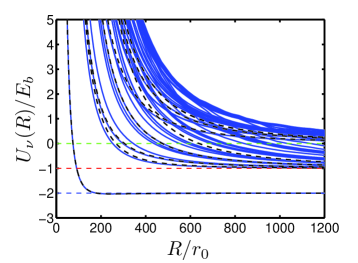
Figure 1: (Color online) Adiabatic hyperspherical potential curves $U_{\nu}(R)$ (solid lines) for two spin-up and two spin-down fermions with an atom-atom scattering length $a_{s}=100r_{0}$. The dashed line at $E=2E_{b}$ (blue online) is the dimer-dimer threshold, the dashed line at $E=E_{b}$ (red online) is the dimer–two-atom threshold, and the dashed line at $E=0$ (green online) is the four-atom threshold. Dashed curves are predictions from Ref. dincao08 .

The development of four-body hyperspherical methods allows, for one thing, an analysis of the full energy dependence of the dimer-dimer scattering length. Figure 1 presents the four-fermion potential curves obtained with the correlated Gaussian hyperspherical method(CGHS). There are three relevant energy thresholds mark with dashed lines in Fig. 1:dimer-dimer threshold at $2E_{b}$, dimer–two-atom threshold at $E_{b}$ and four-atom threshold at 0 energy. The lowest curve represents the dimer-dimer channel and potential curves going asymptotically to $E_{b}$ and 0 represent dimer–two-atom and four-atom channels, respectively. Standard multichannel scattering techniques, like the R-matrix method, can be applied to solve the hyperspherical coupled differential equations. This analysis was performed in a recent study by D’Incao et. al. dincao08 , which obtained the energy dependence of the dimer-dimer scattering length for equal mass systems. Black dashed curves in Figure 1 represent the potential curves of Ref. dincao08 . As we can see, the CGHS method presented here predicts very similar potential curves. The dimer-dimer potential curves obtained with the different methods are almost indistinguishable. For dimer–two-atom potential curves, the CGHS predicts lower potential curves suggesting that the CGHS calculation is slightly better. At large $R$, the asymptotic behavior of both methods agree. This is very encouraging since in the method of D’Incao et. al., the asymptotic behavior of the channel functions is correct by construction, whereas in the CGHS it constitutes an important, nontrivial test. Preliminary calculations with the CGHS potential curves predict a similar energy dependence of the dimer-dimer scattering length. Therefore, the CGHS opens the possibility for accurately analyzing four-body scattering events, as has been carried out for four-interacting bosons in Refs. vonstecher2008fbl ; dincaoDimDim09 .

The calculations of the potential curves at unitarity allows us to extract the four-fermion universal coefficients. As in the $N=3$ system, the potential curves can be written as tan05 ; wern06 ,

$$U_{\nu}(R)=\frac{p_{\nu}^{2}-1/4}{2\mu R^{2}}.$$ (34)

This functional form of the potential curves was verified indirectly in Ref. blumePRL07 by analyzing the spectrum of the four-fermion system under spherical harmonic confinement. It can be shown that all the couplings vanish when the potential curves are proportional to $1/R^{2}$. Therefore the system is described by a set of uncoupled one-dimensional Schrödinger equations that can be solved analytically once the trapping potential is included. These procedure leads to simple expressions for the trapped energies wern06

$$E_{\nu n}=(p_{\nu}+2n+5/2)\hbar\omega.$$ (35)

where $\omega$ is the trapping frequency and we have included the zero point energy of the center-of-mass motion. In Ref. blumePRL07 , the $2\hbar\omega$ spacing was verified and the lowest $p_{\nu}$ coefficients were identified. Equations (34) and (35) are also valid in the non-interacting limit. For $L=0$ and positive parity solutions, the $p_{\nu}^{NI}$ values and their degeneracies $\lambda_{\nu}$ have relatively simple closed forms: $p_{\nu}^{NI}=11/2+2\nu$ and $\lambda_{\nu}=\nu^{4}/96+7\nu^{3}/48+17\nu^{2}/24+133\nu/96+57/64+(-1)^{\nu}\nu/32+7/64(-1)^{\nu}$. Their lowest values can be found in Table 1.

Table 1: Non interacting coefficients $p^{NI}_{\nu}$ of the four-fermion potential curves and their degeneracies $\lambda_{\nu}$.

$\nu$	$p^{NI}_{\nu}$	$\lambda_{\nu}$	$\nu$	$p^{NI}_{\nu}$	$\lambda_{\nu}$
0	11/2	1	5	31/2	50
1	15/2	3	6	35/2	80
2	19/2	8	7	39/2	120
3	23/2	16	8	43/2	175
4	27/2	30	9	47/2	245

The development of the CGHS method allows us to carry out a hyperspherical calculation for the four-fermion problem and to directly verify the form of the hyperspherical potentials. Also, it allows us to analyze deviations from the zero-range solutions due to finite-range effects.

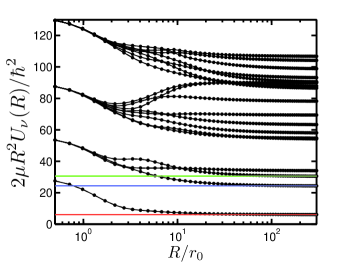
Figure 2: (Color online) Hyperspherical potential curves at unitarity ($a\rightarrow\infty$) for the 4-fermion system multiplied by $2\mu R^{2}/\hbar^{2}$. The solid lines represent the predictions from analyzing the spectrum obtained with the CG method. The symbols correspond to direct evaluation of the potential curves with the CGHS method.

The $20$ lowest four-body potential curves $2\mu R^{2}U_{\nu}(R)/\hbar^{2}$ for the equal-mass system are presented in Figure 2. We can identify three regimes in these potential curves. The region $R\lesssim r_{0}$ is controlled by the kinetic energy. The kinetic energy effects are more important than the interaction energy and the potential curves are well approximated by the non-interacting potential curves. In other words, $2\mu R^{2}U_{\nu}(R)/\hbar^{2}\approx(p^{NI}_{\nu})^{2}-1/4$ and the eigenchannels are well approximated by the hyperspherical harmonics (see Sec. II.2). For that reason, there is a large degeneracy in the $R\lesssim r_{0}$ region which corresponds to the degeneracy of the $\Lambda^{2}$ operator. Furthermore, the potential curves are, to a good approximation, proportional to $1/R^{2}$. The second region is $r_{0}\lesssim R\lesssim 20r_{0}$. In this region both the kinetic and the interaction terms are important and finite range effects are important. In the third region, $R\gtrsim 20r_{0}$, the potential curves recover their universal behavior. The potential curves are, again, approximately proportional to $1/R^{2}$. As $R/r_{0}$ increases, finite-range effects tend to zero and we obtain the zero-range potential curves at unitarity. Therefore, in this region, the eigenvalues of $2\mu R^{2}U_{\nu}(R)/\hbar^{2}$ are approximately $(p^{2}_{\nu}-1/4)$. Thus, we can compare these results with the ones deduced from trapped calculations for $r_{0}/a_{ho}=0.01$ presented in Ref. blumePRL07 . The solid lines correspond to $(p^{2}_{0}-1/4)$, $(p^{2}_{1}-1/4)$ and $(p_{2}^{2}-1/4)$ respectively fnote3 . There is good agreement between the predictions from the trapped system obtained with CG and the direct computation of the potential curves through CGHS.

Table 2: Coefficients $p_{\nu}$ of the four-fermion potential curves.

$\nu$	$p_{\nu}$	$\nu$	$p_{\nu}$	$\nu$	$p_{\nu}$
0	2.509	7	7.959	14	9.502
1	4.944	8	8.341	15	9.648
2	5.529	9	8.848	16	9.938
3	5.846	10	9.292	17	10.205
4	7.363	11	9.366	18	10.339
5	7.402	12	9.5	19	10.482
6	7.621	13	9.501

To quantify this last statement, we analyze the value of $p_{0}$. Several groups stech07 ; chan07 ; vonstechtbp ; alhassid08 ; StetcuCM07 have tried to benchmark the four-body value of $E_{00}$, which is simply related to $p_{0}$. The calculations from Ref. alhassid08 use zero-range interactions explicitly and they report a value of $E_{00}\approx(5.045\pm 0.003)\hbar\omega$. To extract the $p_{0}$ value in the zero-range limit, we carry out two different calculations. First, we study the $E_{00}$ energy obtained with the standard CG method as a function of the range of the two-body interaction and then we extrapolate to zero-range limit. This method was previously applied for the three-body system and the numerical results agreed with the analytical predictions up to 7 digits vonstech08a . The same procedure applied to the four-body system, leads to $p_{0}\approx 2.5096$. The second calculation analyzes the long-range behavior of the potential curves. To eliminate finite-range effects, we extrapolate the potential curve $U_{0}(R)$ to $R/r_{0}\rightarrow\infty$. In this limit, $U_{0}(R)$ is characterized by a value $p_{0}\approx 2.5092$. These two different methods provide a value of $p_{0}$ which agrees in four digits. These values are slightly lower than $p_{0}\approx 2.545\pm 0.003$ predicted in Ref. alhassid08 . This suggests that the uncertainty in Ref. alhassid08 was apparently underestimated.

The calculations of the lowest 20 universal coefficients $p_{\nu}$ is reported in Table 2. It is interesting to note that some of the $p_{\nu}$ coefficients are very similar to the noninteracting coefficients. For example, the $p_{\nu}$ coefficient for $\nu$=12, 13, 14 coincide with noninteracting $p^{NI}_{\nu}$ coefficient. Two of these potential curves are also described by $p_{\nu}=9.5$ in the small $R$ region and deviate from these value in the region $R\sim r_{0}$. These channels have nodes in every spin-up–spin-down interparticle distance, therefore at large distances they recover the noninteracting behavior. The third potential curve smoothly decrease from $p^{NI}_{\nu}=11.5$ at small $R$ to $p_{\nu}=9.5$ at large $R$.

Finally, note that the CGHS method has been successfully applied to the four-boson system vonstecher2008fbl . In that study, the four-boson spectrum is calculated from the CGHS potential curves. Also, that study considers scattering events such as four-body recombination, which was calculated and predicted to be important for the understanding of a recent experiment on Efimov physics in an ultracold Bose gas kraemer2006eeq .

V Conclusions

We have presented an innovative numerical method suitable for the analysis of four-body processes. We have shown several examples for three- and four-particle systems recovering known results. Furthermore, we have obtained the lowest 20 $p_{\nu}$ coefficients for the two-component four-fermion system that characterize both free and trapped systems. These coefficients also characterize the spectrum of four trapped fermions at unitarity. Our results considerably extend previous calculations and provide more accurate energies.

The CGHS method has been used to analyze the four-boson system in Refs. vonstecher2008fbl ; dincaoDimDim09 ; mehtaNbody09 , predicting new phenomena observed experimentally grim4b09 . It has also built a theoretical foundation for the analysis of four-body collisional processes in other systems such as two-component Bose systems papp:040402 ; myatt1997pto ; thalhammer:210402 ; weber2008aud , Bose-Fermi mixtures modugno2002cdf ; inouye2004ohf ; olsen2008cam , and three-component Fermi gasesottenstein:203202 ; huckans2008eri ; blume2008sim . Even though this method was initially implemented to treat ultracold systems using model potentials, it can be in principle extended to other four-body problems.

The authors would like to thank S. T. Rittenhouse, N. P. Mehta and J. P. D’Incao for useful discussions and for providing their four-fermion numerical data (dashed curves included in Fig. 1). This work was supported in part by NSF.

Appendix A Application of Correlated Gaussians to the hyperspherical framework

This appendix illustrates how correlated Gaussian basis functions can be used in the general hyperspherical framework presented in Subsec. II.3. First, we consider the three-particle case and calculate the matrix elements (Eqs. 21, 22 and 29). Then, we discuss how to generate and optimize the basis set.

A.1 Unsymmetrized matrix element evaluation for three particles

In this subsection, we present as an example the evaluation of the matrix elements (Eqs. 21, 22, 29) of three particle system. Consider a system in which the center-of-mass motion decouples. Then, the $L^{P}=0^{+}$ solutions of the body-fixed system can be expanded in terms of the interparticle distances. For the three-body system the correlated basis functions take the form

$$\Psi_{A}(r_{12},r_{13},r_{23})=\exp\left[-\left(\frac{r_{12}^{2}}{2d_{12}^{2}}+\frac{r_{13}^{2}}{2d_{13}^{2}}+\frac{r_{23}^{2}}{2d_{23}^{2}}\right)\right].$$ (36)

For equal mass systems, we can write Eq.(36) in terms of the following Jacobi coordinates:

$$\mathbf{x_{1}}=\frac{1}{\sqrt{2}}(\mathbf{r}_{1}-\mathbf{r}_{2}),$$ (37)

$$\mathbf{x_{2}}=\sqrt{\frac{2}{3}}\left(\mathbf{r}_{3}-\frac{\mathbf{r}_{1}+\mathbf{r}_{2}}{2}\right).$$ (38)

The basis functions [Eq. (36)] can be written as

$$\Psi_{A}(r_{12},r_{13},r_{23})=\mathinner{\langle{\mathbf{x_{1}},\mathbf{x_{2}}|A}\rangle}=\exp(-\frac{\mathbf{x}^{T}.A.\mathbf{x}}{2})\\ =\exp(-\frac{\mathbf{x_{1}}.\mathbf{x_{1}}a_{11}+2\mathbf{x_{1}}.\mathbf{x_{2}}a_{12}+\mathbf{x_{2}}.\mathbf{x_{2}}a_{22}}{2})$$ (39)

where $\mathbf{x}\equiv\{\mathbf{x}_{1},\mathbf{x}_{2}\}$ and $A$ is a 2 by 2 symmetric matrix whose elements are $a_{11}=2/d_{12}^{2}+1/2(1/d_{13}^{2}+1/d_{23}^{2})$ , $a_{12}=a_{21}=\sqrt{3}/2(1/d_{23}^{2}-1/d_{13}^{2})$, and $a_{22}=3/2(1/d_{13}^{2}+1/d_{23}^{2})$. In Eq. (39), we can clearly see that the state $\mathinner{\langle{\mathbf{x_{1}},\mathbf{x_{2}}|A}\rangle}$ depends only on the distances $x_{1}$, and $x_{2}$ plus the angle $\theta_{12}$ between them, $\cos\theta_{12}=\mathbf{x_{1}}.\mathbf{x_{2}}/x_{1}x_{2}$.

We want to obtain the matrix elements corresponding to these basis functions at fixed hyperradius $R$. We define the hyperradius to be $R^{2}=\mathbf{x}_{1}^{2}+\mathbf{x}_{2}^{2}$. The integrand of the overlap matrix element between $\mathinner{|{A}\rangle}$ and $\mathinner{|{B}\rangle}$, noted as $B.A$, is

$$B.A=\exp(-\frac{\mathbf{x}^{T}.(A+B).\mathbf{x}}{2}).$$ (40)

We change to the Jacobi basis set that diagonalizes $A+B$ and we call $\beta_{1}$ and $\beta_{2}$ the eigenvalues and $\mathbf{y}\equiv\{\mathbf{y}_{1},\mathbf{y}_{2}\}$ the orthonormal eigenvectors. In this new coordinate basis, Eq. (40) has a simple form,

$$B.A=\exp(-\frac{\beta_{1}y_{1}^{2}+\beta_{2}y_{2}^{2}}{2}).$$ (41)

We integrate over the angles of the vectors $\mathbf{y}_{1}$ and $\mathbf{y}_{2}$ and we fix the hyperradius, so $y_{1}=R\cos\theta$ and $y_{2}=R\sin\theta$. In this set of coordinates, the matrix element at fixed $R$ is

$$\mathinner{\langle{B|A}\rangle}\Big{|}_{R}=(4\pi)^{2}\int_{0}^{\pi/2}e^{-R^{2}(\beta_{1}\cos^{2}\theta+\beta_{2}\sin^{2}\theta)/2}\cos^{2}\theta\sin^{2}\theta d\theta$$ (42)

This integration has a closed-form result,

$$\mathinner{\langle{B|A}\rangle}\Big{|}_{R}=2\pi^{3}\frac{\exp(-\frac{\beta_{1}+\beta_{2}}{4}R^{2})}{\xi}I_{1}\left(\xi\right).$$ (43)

Here we have introduced the definition $\xi=R^{2}(\beta_{1}-\beta_{2})/4$.

To simplify the interaction matrix element evaluation, we can adopt a Gaussian model potential as was utilized in the CG method. In this case, the interaction term can be evaluated in the same way we have calculated the overlap term since the interaction is also a Gaussian. Each pairwise interaction can be easily written as $V_{ij}=V_{0}\exp(-\frac{r_{ij}^{2}}{2r_{0}^{2}})=V_{0}\exp(-\mathbf{x}^{T}.M^{(ij)}.\mathbf{x}/(2r_{0}^{2}))$. Therefore, to calculate the interaction matrix element, we need to evaluate

$$\mathinner{\langle{B|V_{ij}|A}\rangle}=V_{0}\int d\Omega\exp(-\frac{\mathbf{x}^{T}.(A+B+M^{(ij)}/r_{0}^{2}).\mathbf{x}}{2}).$$ (44)

This integration can be done following the same steps of the overlap matrix element. Equation (43) can be used directly if we multiply it by $V_{0}$, and $\beta_{1}$ and $\beta_{2}$ are replaced by the eigenvalues of $A+B+M^{(ij)}/r_{0}^{2}$. Note that for each pairwise interaction (and for each pair of basis functions in the matrix element), the matrix $M^{(ij)}$ changes and requires a new evaluation of the eigenvalues.

The third term we need to evaluate is the hyperangular kinetic term at fixed $R$. This kinetic term is proportional to the grand angular momentum operator $\Lambda$ defined for the $N=3$ case as

$$\frac{\Lambda^{2}\hbar^{2}}{2\mu R^{2}}=-\sum_{i}\frac{\hbar^{2}\nabla_{i}^{2}}{2\mu}+\frac{\hbar^{2}}{2\mu}\frac{1}{R^{5}}\frac{\partial}{\partial R}R^{5}\frac{\partial}{\partial R}.$$ (45)

The expression can be formally written as

$$\mathcal{T}_{\Omega}=\mathcal{T}_{T}-\mathcal{T}_{R},$$ (46)

where

$$\mathcal{T}_{\Omega}=\frac{\Lambda^{2}\hbar^{2}}{2\mu R^{2}},\;\;\;\;\mathcal{T}_{T}=-\sum_{i}\frac{\hbar^{2}\nabla_{i}^{2}}{2\mu},$$ (47)

and

$$\mathcal{T}_{R}=-\frac{\hbar^{2}}{2\mu}\frac{1}{R^{5}}\frac{\partial}{\partial R}R^{5}\frac{\partial}{\partial R}.$$ (48)

In typical calculations, $\mathcal{T}_{\Omega}$ is evaluated by directly applying the corresponding derivatives in the hyperangles $\Omega$. However, in this case, it is convenient to evaluate $\mathcal{T}_{T}$ and $\mathcal{T}_{R}$ separately, and make use of (46).

The integrand of the total kinetic term $\mathcal{T}_{T}$ takes the form

$$B|\mathcal{T}_{T}|A=\exp(-\frac{\mathbf{x}^{T}.B.\mathbf{x}}{2})\left(-\sum_{i}^{2}\frac{\hbar^{2}}{2\mu}\nabla^{2}_{i}\right)\exp(-\frac{\mathbf{x}^{T}.A.\mathbf{x}}{2}).$$ (49)

First, we diagonalize $A$ and use the eigenvectors and eigenvalues of $A$, obtaining,

$$B|\mathcal{T}_{T}|A=-\frac{\hbar^{2}}{2\mu}\left(-\mbox{Tr}[A]+\mathbf{x}^{T}.A^{2}.\mathbf{x}\right)\exp(-\frac{\mathbf{x}^{T}.(A+B).\mathbf{x}}{2}).$$ (50)

Here Tr is the trace function. We can use $\mbox{Tr}[A]=(\alpha_{1}+\alpha_{2})$, where $\alpha_{1}$ and $\alpha_{2}$ are the eigenvalues of $A$. Now we diagonalize $A+B$. We call $T$ the matrix with the orthonormal eigenstates in columns and $\beta_{1}$ and $\beta_{2}$ are the eigenvalues of $A+B$. We make a change of coordinates to the basis set that diagonalizes $A+B$. We obtain

$$B|\mathcal{T}_{T}|A=-\frac{\hbar^{2}}{2\mu}\left(-3(\alpha_{1}+\alpha_{2})+\mathbf{y}.G.\mathbf{y}\right)\exp(-\frac{\beta_{1}y_{1}^{2}+\beta_{2}y_{2}^{2}}{2}),$$ (51)

where $G=T^{T}.A^{2}.T$, and $\mathbf{y}_{1}$ and $\mathbf{y}_{2}$ are the vectors in the new eigen basis. The integration over the angles of these vectors is trivial. After this integration, we fix the hyperradius and integrate over the hyperangle $\theta$ defined by $y_{1}=R\cos\theta$ and $y_{2}=R\sin\theta$,

$$\mathinner{\langle{B|\mathcal{T}_{T}|A}\rangle}\Big{|}_{R}=-\frac{(4\pi)^{2}\hbar^{2}}{2\mu}\int_{0}^{\pi/2}\Big{[}-3(\alpha_{1}+\alpha_{2})\\ +g_{11}R^{2}\cos^{2}\theta+g_{22}R^{2}\sin^{2}\theta\Big{]}\\ \exp(-\frac{\beta_{1}R^{2}\cos^{2}\theta+\beta_{2}R^{2}\sin^{2}\theta}{2})\cos^{2}\theta\sin^{2}\theta d\theta.$$ (52)

This integration can be done analytically and the results expressed in terms of the Bessel functions $I_{1}$ and $I_{0}$:

$$\mathinner{\langle{B|\mathcal{T}_{T}|A}\rangle}\Big{|}_{R}=-\frac{\hbar^{2}e^{-\frac{(\beta_{1}+\beta_{2})R^{2}}{2}}\pi^{3}R^{2}}{16\xi\mu}\\ \left\{-8(g_{11}-g_{22})I_{0}\left[\xi\right]+\frac{2}{\xi}\Big{\{}8(g_{11}-g_{22})\right.\\ \left.+(\beta_{1}-\beta_{2})\left(-6(\alpha_{1}+\alpha_{2})+(g_{11}+g_{22})R^{2}\right)\Big{\}}I_{1}\left[\xi\right]\right\}.$$ (53)

Now we will evaluate $\mathcal{T}_{R}$, the hyperradial kinetic term. It is written as

$$\mathcal{T}_{R}=-\frac{\hbar^{2}}{2\mu}\left(\frac{1}{R^{5/2}}\frac{\partial^{2}}{\partial R^{2}}R^{5/2}-\frac{15}{4R^{2}}\right).$$ (54)

Therefore, the integrand takes the form

$$B|\mathcal{T}_{R}|A=-\frac{\hbar^{2}}{2\mu}\exp(-\frac{\mathbf{x}^{T}.B.\mathbf{x}}{2})\\ \left(\frac{1}{R^{5/2}}\frac{\partial^{2}}{\partial R^{2}}R^{5/2}-\frac{15}{4R^{2}}\right)\exp\left(-\frac{\mathbf{x}^{T}.A.\mathbf{x}}{2}\right),$$ (55)

We use the property $\mathbf{x}^{T}.A.\mathbf{x}=R^{2}F_{A}(\Omega)$ to evaluate the derivatives with respect to $R$. This allows a simple calculation of the derivatives in Eq. (55), yielding

$$B|\mathcal{T}_{R}|A=\frac{\hbar^{2}}{2\mu R^{2}}\left[6\mathbf{x}^{T}.A.\mathbf{x}-(\mathbf{x}^{T}.A.\mathbf{x})^{2}\right]e^{-\mathbf{x}^{T}.(A+B).\mathbf{x}/2}.$$ (56)

Next we diagonalize $A+B$, and set $D=T^{T}.A.T$, giving

$$B|\mathcal{T}_{R}|A=\frac{\hbar^{2}}{2\mu R^{2}}\left[6\mathbf{y}.D.\mathbf{y}-(\mathbf{y}.D.\mathbf{y})^{2}\right]\exp\left(-\frac{\beta_{1}y_{1}^{2}+\beta_{2}y_{2}^{2}}{2}\right)$$ (57)

The terms $\mathbf{y}.D.\mathbf{y}$ and $(\mathbf{y}.D.\mathbf{y})^{2}$ depend on the polar angles of the vectors. The integration over the polar angles ($\Omega_{1}=\{\phi_{1},\theta_{1}\}$ and $\Omega_{2}=\{\phi_{2},\theta_{2}\}$) of these terms is

$$\int\left[6\mathbf{y}.D.\mathbf{y}-(\mathbf{y}.D.\mathbf{y})^{2}\right]d\Omega_{1}d\Omega_{2}=(4\pi)^{2}\Big{\{}6d_{11}y_{1}^{2}+6d_{22}y_{2}^{2}\\ -\big{[}d_{11}^{2}y_{1}^{4}+(2d_{11}d_{22}+4d_{12}^{2}/3)y_{1}^{2}y_{2}^{2}+d_{22}^{2}y_{2}^{4}\big{]}\Big{\}}.$$ (58)

Now we carry out the integration over the hyperangle $\theta$, using $y_{1}=R\cos\theta$ and $y_{2}=R\sin\theta$, which gives

$$\mathinner{\langle{B|\mathcal{T}_{R}|A}\rangle}\Big{|}_{R}=\frac{(4\pi)^{2}\hbar^{2}}{2\mu R^{2}}\int_{0}^{\pi/2}\Big{\{}6d_{11}R^{2}\cos^{2}\theta\\ +6d_{22}R^{2}\sin^{2}\theta-d_{11}^{2}R^{4}\cos^{4}\theta\\ -(2d_{11}d_{22}+4d_{12}^{2}/3)R^{4}\cos^{2}\theta\sin^{2}\theta-d_{22}^{2}R^{4}\sin^{4}\theta\Big{\}}\\ \exp\left(-\frac{\beta_{1}R^{2}\cos^{2}\theta+\beta_{2}R^{2}\sin^{2}\theta}{2}\right)\cos^{2}\theta\sin^{2}\theta d\theta.$$ (59)

This integration has the analytical form

$$\mathinner{\langle{B|\mathcal{T}_{R}|A}\rangle}\Big{|}_{R}=-\frac{\hbar^{2}}{\mu}\frac{e^{-\frac{(\beta_{1}+\beta_{2})R^{2}}{4}}\pi^{3}R^{2}}{64\xi^{2}}\Big{\{}-8\Big{[}-8d_{12}^{2}\\ +(d_{11}-d_{22})\big{(}6(-\beta_{1}+\beta_{2}+d_{11}-d_{22})+\\ 4\xi(d_{11}+d_{22})\big{)}\Big{]}I_{0}[\xi]+\frac{2}{\xi}\Big{[}-64d_{12}^{2}+\\ 48(d_{11}-d_{22})(-\beta_{1}+\beta_{2}+d_{11}-d_{22})\\ +8\xi(-3\beta_{1}+3\beta_{2}+4d_{11}-4d_{22})(d_{11}+d_{22})\\ \left.+16\xi^{2}(d_{11}^{2}+d_{22}^{2})\Big{]}I_{1}[\xi]\right\}.$$ (60)

Combining Eqs. (53, 60), we obtain $\mathcal{T}_{\Omega}$. The expression for $\mathcal{T}_{\Omega}$ can be simplified using the relation $G=D^{2}$ to write $G$ matrix elements of Eq. (53) in terms of the ones of $D$. This same procedure can be applied to extract the $P$ and $\tilde{Q}$ matrix elements:

$$\mathinner{\langle{B|\frac{\partial A}{\partial R}}\rangle}\Big{|}_{R},\,\,\,\mbox{and}\,\,\,\,\mathinner{\langle{\frac{\partial B}{\partial R}|\frac{\partial A}{\partial R}}\rangle}\Big{|}_{R}.$$ (61)

A useful test to verify the functional form of the matrix elements is to integrate them with respect to $R$, with the corresponding volume element, and compare that result with the standard CG matrix elements. Another important test is to verify that $\mathcal{T}_{\Omega}$ is symmetric under the exchange of the basis functions $A$ and $B$. This is not a trivial test since neither $\mathcal{T}_{T}$ nor $\mathcal{T}_{R}$ are symmetric.

A major advantage of these matrix element evaluations is that they can be easily extended to four particles. In general, these matrix elements evaluations would require a 5-D numerical integration but for these basis functions, with the above analytical development, they only require a 1-D numerical integration.

A.2 General considerations

Many of the procedures of the standard CG method can be easily extended to the CGHS. The selection, symmetrization, and optimization of a basis follow the same ideas of the standard CG method. However, the evaluation of the unsymmetrized matrix elements at fixed $R$ is clearly different. Furthermore, the hyperangular Hamiltonian [Eq. 17] need to solved at different hyperradius $R$.

There are several properties that make this method particularly efficient. For the model potential used, the scattering length is tuned by varying the potential depths of the two-body interaction. Therefore, as in the CG case, the matrix elements need only be calculated once; then they can be used for a wide range of scattering lengths. Of course, the basis set should be complete enough to describe the relevant potential curves at all the desired scattering length values.

The selection of the basis function generally depends on $R$. To avoid numerical problems, the mean hyperradius of each basis function $\mathinner{\langle{R}\rangle}_{B}$ should be comparable to the hyperradius $R$ in which the matrix elements are evaluated. We can ensure that $\mathinner{\langle{R}\rangle}_{B}\sim R$ by selecting some (or all) the weights $d_{ij}$ to be of the order of $R$.

We consider two different optimization procedures. The first possible optimization procedure is the following: First, we select a few basis functions and optimize them to describe the lowest hyperspherical harmonics. The Gaussian widths of these basis functions are rescaled by $R$ at each hyperradius so that they represent the hyperspherical harmonics equally well. These basis functions are used at all $R$, while the remaining are optimized at each $R$. Starting from small $R$ (of the order of the range of the potential), we optimize a set of basis functions. As $R$ is increased, the basis set is increased and reoptimized. At every $R$ step, only a fraction of the basis set is optimized, and those basis functions are selected randomly. After a several $R$-steps, the basis set is increased.

Instead of optimizing the basis set at each $R$, one can alternatively try to create a complete basis set at large $R_{max}$. In this case, the basis functions should be complete enough to describe the lowest channel functions with interparticle distances varying from interaction range $r_{0}$ up to the hyperradius $R_{max}$. Such a basis set can be rescaled to any $R<R_{max}$ and should efficiently describe the channel functions at that $R$. The rescaling procedure is simply $d_{ij}/R=d_{ij}^{max}/R_{max}$. This procedure avoids the optimization at each $R$. Furthermore, the kinetic, overlap, and couplings matrix elements at $R$ are straightforwardly related with the ones at $R_{max}$. So, the interaction potential is the only matrix element that needs to be recalculated at each $R$. This property can be understood using dimensional analysis. The kinetic, overlap, and coupling matrix elements only depend on $R$, so a rescaling of the widths is simply related to a rescaling of the matrix elements. In contrast, the interaction potential introduces a new length scale, so the matrix elements depend on both $R$ and $r_{0}$, and the rescaling does not work.

These two methods, the “complete basis set” or the “small optimized basis set” method, can be appropriate in different circumstances. If a large number of channels are needed, probably the complete basis method is the best choice. But, if only a couple of particular channel potential curves and couplings are needed, then the small optimized basis set method might be more efficient.

The most convenient strategy we have found for optimizing the basis function in the four-boson and four-fermion problems is the following: First we select an hyperradius $R_{m}$ that is $R_{m}\approx 300\,r_{0}$ where the basis function will be initially optimized. The basis set is increased and optimized until the relevant potential curves are converged and, in that sense, the basis is complete. This basis is then rescaled, as proposed in the second optimization method, to all $R<R_{m}$. For $R>R_{m}$, it is too expensive to have a “complete” basis set. For that reason, we use the “small optimized basis set” method which allows a reliable description of the lowest potential curves.

Note that for standard correlated Gaussian calculations, the matrices $A$ and $B$ need to be positive definite. This condition restricts the Hilbert space to exponentially decaying functions. In the hyperspherical treatment, this is not necessary since the matrix elements can always be calculated at fixed $R$, as the integrals converge even for exponentially growing functions. This gives more flexibility in choosing the optimal basis functions.

References

- (1) E. Braaten and H. W. Hammer, Phys. Rep. 428, 259 (2006).
- (2) V. Efimov, Yad. Fiz. 12, 1080 (1970 [Sov. J. Nucl. Phys. 12, 589 (1971)]).
- (3) B. D. Esry, C. H. Greene, and J. P. Burke Jr, Phys. Rev. Lett. 83, 1751 (1999).
- (4) T. Kraemer, M. Mark, P. Waldburger, J. G. Danzl, C. Chin, B. Engeser, A. D. Lange, K. Pilch, A. Jaakkola, H. C. Naegerl, et al., Nature 440, 315 (2006).
- (5) D. M. Eagles, Phys. Rev. 186, 456 (1969).
- (6) A. J. Leggett, in “Modern Trends in the Theory of Condensed Matter”, ed. by A. Pekalski J. Przystawa, Springer, Berlin (1980).
- (7) P. Nozières and S. Schmitt-Rink, J. Low Temp. Phys. 59, 195 (1985).
- (8) M. Greiner, C. A. Regal, and D. S. Jin, Nature 426, 537 (2003).
- (9) S. Jochim, M. Bartenstein, A. Altmeyer, G. Hendl, S. Riedl, C. Chin, J. Hecker Denschlag, and R. Grimm, Science 302, 2101 (2003).
- (10) M. W. Zwierlein, C. A. Stan, C. H. Schunck, S. M. F. Raupach, S. Gupta, Z. Hadzibabic, and W. Ketterle, Phys. Rev. Lett. 91, 250401 (2003).
- (11) T. Bourdel, L. Khaykovich, J. Cubizolles, J. Zhang, F. Chevy, M. Teichmann, L. Tarreell, S. J. J. M. F. Kokkelmans, and C. Salomon, Phys. Rev. Lett. 93, 050401 (2004).
- (12) C. A. Regal, M. Greiner, and D. S. Jin, Phys. Rev. Lett. 92, 40403 (2004).
- (13) M. W. Zwierlein, C. A. Stan, C. H. Schunck, S. M. F. Raupach, A. J. Kerman, and W. Ketterle, Phys. Rev. Lett. 92, 120403 (2004).
- (14) M. W. Zwierlein, J. R. Abo-Shaeer, A. Schirotzek, C. H. Schunck, and W. Ketterle, Nature 435, 1047 (2005).
- (15) D. Jaksch, C. Bruder, J. Cirac, C. Gardiner, and P. Zoller, Phys. Rev. Lett. 81, 3108 (1998).
- (16) B. Paredes, A. Widera, V. Murg, O. Mandel, S. Fölling, I. Cirac, G. Shlyapnikov, T. Hänsch, I. Bloch, and N. Contact, Nature 429, 277 (2004).
- (17) T. Kinoshita, T. Wenger, and D. Weiss, Science 305, 1125 (2004).
- (18) I. Bloch, J. Dalibard, and W. Zwerger, Rev. Mod. Phys. 80, 885 (2008).
- (19) D. S. Petrov, Phys. Rev. Lett. 93, 143201 (2004).
- (20) D. S. Petrov, Phys. Rev. A 67, 010703 (2003).
- (21) D. S. Petrov, C. Salomon, and G. V. Shlyapnikov, Phys. Rev. Lett. 93, 90404 (2004).
- (22) A. Deltuva and A. Fonseca, Phys. Rev. Lett. 98, 16 (2007).
- (23) J. von Stecher and C. H. Greene, Phys. Rev. Lett. 99, 090402 (2007).
- (24) J. P. D’Incao, S. T. Rittenhouse, N. P. Mehta, and C. H. Greene, Phys. Rev. A 79, 030501 (2009).
- (25) Y. Wang and B. Esry, Phys. Rev. Lett. 102, 133201 (2008).
- (26) L. D. Faddeev, Zh. Eksp. Teor. Fiz 39, 1459 (1960).
- (27) Y. Suzuki and K. Varga, Stochastic Variational Approach to Quantum-Mechanical Few-Body Problems (Springer-Verlag, Berlin, 1998).
- (28) R. A. Malfliet and J. A. Tjon, Nucl. Phys. A 127, 161 (1969).
- (29) O. A. Yakubovsky, Yad. Fiz. 5, 1312 (1967 [Sov. J. Nucl. Phys. 5 937 (1967)]).
- (30) J. Macek, J. Phys. B 1, 831 (1968).
- (31) K. Singer, Proc. R. Soc. London, Ser. A 258, 412 (1960).
- (32) S. F. Boys, Proc. R. Soc. London, Ser. A 258, 402 (1960).
- (33) V. I. Kukulin and V. Krasnopol’sky, J. Phys. G 3, 795 (1977).
- (34) K. Varga and Y. Suzuki, Phys. Rev. A 53, 1907 (1996).
- (35) K. Varga and Y. Suzuki, Phys. Rev. C 52, 2885 (1995).
- (36) K. Varga and Y. Suzuki, Comp. Phys. Comm. 106, 157 (1997).
- (37) K. Varga, Y. Suzuki, and R. G. Lovas, Nucl. Phys. A 571, 447 (1994).
- (38) D. Blume, J. von Stecher, and C. H. Greene, Phys. Rev. Lett. 99, 233201 (2007).
- (39) J. von Stecher and C. Greene, Phys. Rev. A 75, 22716 (2007).
- (40) J. von Stecher, C. H. Greene, and D. Blume, Phys. Rev. A 77, 043619 (2008).
- (41) L. M. Delves, Nucl. Phys. 9, 391 (1959).
- (42) L. M. Delves, Nucl. Phys. 20, 275 (1960).
- (43) C. D. Lin, Phys. Rep. 257, 1 (1995).
- (44) Y. F. Smirnov and K. V. Shitikova, Sov. J. Part. Nucl. 8, 44 (1977).
- (45) X. Chapuisat, Phys. Rev. A 45, 4277 (1992).
- (46) M. Aymar, C. H. Greene, and E. Luc-Koenig, Rev. Mod. Phys. 68, 1015 (1996).
- (47) O. Zatsarinny and K. Bartschat, J. Phys. B 37, 2173 (2004).
- (48) A. Sunderland, C. Noble, V. Burke, and P. Burke, Comp. Phys. Commun. 145, 311 (2002).
- (49) R. T. Pack and G. A. Parker, J. Chem. Phys. 87, 3888 (1987).
- (50) Y. Zhou, C. D. Lin, and J. Shertzer, J. Phys. B 26, 3937 (1993).
- (51) B. D. Esry, C. D. Lin, and C. H. Greene, Phys. Rev. A 54, 394 (1996).
- (52) H. Suno, B. D. Esry, C. H. Greene, and J. P. Burke Jr, Phys. Rev. A 65, 42725 (2002).
- (53) F. Werner and Y. Castin, Phys. Rev. A 74, 053604 (2006).
- (54) S. Y. Chang and G. F. Bertsch, Phys. Rev. A 76, 021603 (R) (2007).
- (55) J. von Stecher, C. H. Greene, and D. Blume, Phys. Rev. A 76, 053613 (2007).
- (56) Y. Alhassid, G. F. Bertsch, and L. Fang, Phys. Rev. Lett. 100, 230401 (2008).
- (57) I. Stetcu, B. R. Barrett, U. van Kolck, and J. P. Vary, Phys. Rev. A 76, 063613 (2007).
- (58) H. H. Sørensen, D. V. Fedorov, and A. S. Jensen, Workshop on Nuclei and Mesoscopic Physics: WNMP 2004. AIP Conference Proceedings, 777, 12 (2005).
- (59) H. H. Sørensen, Arxiv preprint cond-mat/0502126 (Master Thesis) (2005).
- (60) U. Fano, Phys. Rev. A 24, 2402 (1981).
- (61) Even though is arbitrary, there is one preferable selection: that conserves the volume element of the coordinate transformation.Delves60 In this article, we will only present results for equal mass systems for which is simpler to simply choose .
- (62) H. T. Coelho and J. E. Hornos, Phys. Rev. A 43, 6379 (1991).
- (63) N. P. Mehta, S. T. Rittenhouse, J. P. D’Incao, and C. H. Greene, Arxiv preprint arXiv:0706.1296 (2007).
- (64) The (3N-7) numerical integration results from the following reasoning: initially we have 3N numerical integration but 3 dimensions are removed by decoupling the center of mass motion, 3 dimension are removed fixing the Euler angles and 1 dimension is removed by fixing R.
- (65) J. von Stecher, Ph.D. thesis, University of Colorado, 2008 available at http://jilawww.colorado.edu/pubs/thesis/ vonstecher/von_stecher_thesis.pdf.
- (66) J. Macek, Z. Phys. D 3, 31 (1986).
- (67) D. Blume and C. H. Greene, J. Chem. Phys. 112, 8053 (2000).
- (68) J. von Stecher, J. P. D’Incao, and C. H. Greene, eprint arXiv: 0810.3876 (2008), Nat. Phys. (to appear).
- (69) J. P. D’Incao, J. von Stecher, and C. H. Greene, Arxiv preprint arXiv:0903.3348 (2009).
- (70) S. Tan, Arxiv preprint cond-mat/0412764 (2004).
- (71) The coefficients can be easily related with the of Ref. blumePRL07 by .
- (72) N. P. Mehta, S. T. Rittenhouse, J. P. D’Incao, J. von Stecher, and C. H. Greene, Arxiv preprint arXiv:0903.4145 (2009).
- (73) F. Ferlaino, S. Knoop, M. Berninger, W. Harm, H.-C. D’Incao, J. P. Nägerl, and R. Grimm, Phys. Rev. Lett. 102, 140401 (2009).
- (74) S. B. Papp, J. M. Pino, and C. E. Wieman, Phys. Rev. Lett. 101, 040402 (2008).
- (75) C. J. Myatt, E. A. Burt, R. W. Ghrist, E. A. Cornell, and C. E. Wieman, Phys. Rev. Lett. 78, 586 (1997).
- (76) G. Thalhammer, G. Barontini, L. D. Sarlo, J. Catani, F. Minardi, and M. Inguscio, Phys. Rev. Lett. 100, 210402 (2008).
- (77) C. Weber, G. Barontini, J. Catani, G. Thalhammer, M. Inguscio, and F. Minardi, Phys. Rev. A 78, 061601(R) (2008).
- (78) G. Modugno, G. Roati, F. Riboli, F. Ferlaino, R. Brecha, and M. Inguscio, Science 297, 2240 (2002).
- (79) S. Inouye, J. Goldwin, M. L. Olsen, C. Ticknor, J. L. Bohn, and D. S. Jin, Phys. Rev. Lett. 93, 183201 (2004).
- (80) M. L. Olsen, J. D. Perreault, T. D. Cumby, and D. S. Jin, Arxiv preprint arXiv:0810.1965 (2008).
- (81) T. B. Ottenstein, T. Lompe, M. Kohnen, A. N. Wenz, and S. Jochim, Phys. Rev. Lett. 101, 203202 (2008).
- (82) J. H. Huckans, J. R. Williams, E. L. Hazlett, R. W. Stites, and K. M. O’Hara, Arxiv preprint arXiv:0810.3288 (2008).
- (83) D. Blume, S. T. Rittenhouse, J. von Stecher, and C. H. Greene, Phys. Rev. A 77, 33627 (2008).