Discovery of 5000 Active Galactic Nuclei behind the Magellanic Clouds

Abstract

We show that using mid-IR color selection to find Active Galactic Nuclei (AGNs) is as effective in dense stellar fields such as the Magellanic Clouds as it is in extragalactic fields with low stellar densities using comparisons between the Spitzer Deep, Wide-Field Survey data for the NOAO Deep Wide Field Survey Böotes region and the SAGE Survey of the Large Magellanic Cloud. We use this to build high purity catalogs of $\sim 5000$ AGN candidates behind the Magellanic Clouds. Once confirmed, these quasars will expand the available astrometric reference sources for the Clouds and the numbers of quasars with densely sampled, long-term ($>$decade) monitoring light curves by well over an order of magnitude and potentially identify sufficiently bright quasars for absorption line studies of the interstellar medium of the Clouds.

1. Introduction

At a first glance, searching for quasars behind the disk of the Galaxy or the Magellanic Clouds seems neither useful nor promising. While this presently holds for the problem of finding such quasars, they are useful tools once discovered. In particular, they serve as astrometric references for proper motion studies and the (ultraviolet) bright quasars can be used to study absorption in the interstellar medium. They may also be unique tools for studying the variability of quasars. After outlining the uses of such quasars and the results of existing searches for them, we present a simple, robust procedure to identify quasars in dense stellar fields with moderate extinction and generate a high purity catalog of quasar candidates in the Magellanic Clouds.

Our understanding of the dynamics of the Galaxy and the Large and Small Magellanic Clouds (LMC and SMC) relies profoundly on our ability to measure the proper motions of stars, and a key use of quasars in dense stellar fields is as astrometric references. After early efforts using ground based imaging in the Magellanic Clouds (e.g., Jones et al. 1994; Anguita et al. 2000; Drake et al. 2001; Pedreros et al. 2002) and the Galactic Bulge (e.g., Spaenhauer et al. 1992; Rattenbury et al. 2007; Vieira et al. 2007), most recent studies have used the higher astrometric precision of the Hubble Space Telescope (HST). This has led to considerable recent progress on the proper motions of stars in the LMC (Kallivayalil et al. 2006a; Piatek et al. 2008; Pedreros et al. 2006), SMC (Kallivayalil et al. 2006b) and the Galactic bulge (Kuijken & Rich 2002; Kozłowski et al. 2006; Clarkson et al. 2008). These studies are limited by the small numbers of available quasars, with less than 100 known for the LMC (e.g., Eyer 2002; Geha et al. 2003; Dobrzycki et al. 2002, 2005) and only a few dozen candidates behind the Galactic Bulge (e.g., Sumi et al. 2005).

A second use for these quasars is for absorption line studies of the interstellar medium of the Galaxy and the Clouds (e.g., Shull et al. 2000; Savage et al. 2000). For the Clouds this has largely been limited to studies of the Magellanic Stream (e.g., Sembach et al. 2000; Smoker et al. 2005; Lehner et al. 2008; Misawa et al. 2009) rather than the Clouds themselves. While there are no guarantees that sufficiently bright quasars exist behind the Clouds, the advent of the Cosmic Origins Spectrograph for HST will allow the use of significantly fainter quasars than earlier studies.

The third, and least obvious, use of these quasars is as the best existing data base for understanding quasar variability. Because of the microlensing studies of the Magellanic Clouds and the Galactic bulge (EROS – Afonso et al. 1999; MACHO – Alcock et al. 2000; MOA – Bond et al. 2001; OGLE – Udalski 2003), most quasars identified in these regions will have well-sampled, decade long light curves that can be used to study the optical variability of quasars. The ensemble variability of quasars is well studied (e.g., de Vries et al. 2003; Vanden Berk et al. 2004), but less is known about the variability properties of individual quasars because it has been difficult to monitor them in large numbers. While some newer projects will remedy this problem (e.g., QUEST, Ringstorf et al. 2009; Pan-STARRS, LSST), these data already exist for quasars in the microlensing regions and, to a lesser extent, for Stripe 82 of the Sloan Digital Sky Survey (SDSS, Bramich et al. 2008). For example, Kelly et al. (2009), recently found that quasar light curves have characteristic time scales that are well-correlated with their black hole mass (estimated from their emission line widths), but poorly correlated with their accretion rate (relative to Eddington). A significant fraction of the quasars suitable for the analysis were the Geha et al. (2003) variability-selected quasars in the LMC.

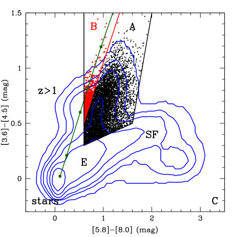
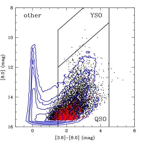
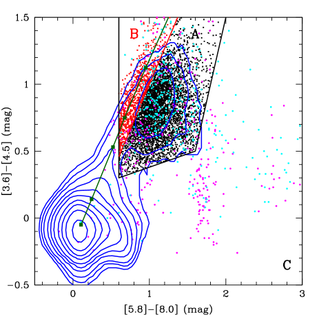
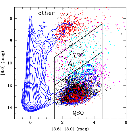
Figure 1.— $[3.6]-[4.5]$/$[5.8]-[8.0]$ color-color distribution (left) and $[3.6]-[8.0]$/$[8.0]$ CMD (right) of the extragalactic SDWFS. The smoothed contours are for 2, 10, 20, 50, 100 and 200 objects per bin with 0.1 mag bins for the colors and $0.2$ mag bins for the magnitude. In the left panel we indicate the typical source type for the different color regions (stars, E – ellipticals, SF – star forming galaxies and $z>1$ galaxies). We also show the Stern et al. (2005) AGN wedge and the color locus of black bodies (green curve marked with squares for temperatures of 1500, 1300, 1000, 800 and 600 K). In the right panel we show the boundaries of our YSO and quasi-stellar objects (QSO) selection regions (Cut #2). The points are the AGN wedge objects, colored black if in region A and red if in region B (Cut #1). In the CMD, the region B AGN tend to be somewhat fainter than the region A AGN. Few quasars lie in the YSO region, but this includes the brightest objects.

Figure 2.— The same distributions as in Figure 2 but for the SAGE point source catalogs. The smoothed contours are for 2, 5, 10, 20, 50, 100, 200, 500, 1000 and 2000 objects per bin where the bin sizes are unchanged. The black and red points again mark class A and B objects in the AGN wedge, but we now see that class B objects are also found on the AGB sequence, but at apparent magnitudes very different from those of AGN. In both panels we also show confirmed (magenta) and highly probable (cyan) YSOs from Whitney et al. (2008). Many of these objects lie in the AGN wedge (478 of 722), and of those in the AGN wedge 184 (191) are in the QSO (YSO) region.

Most quasars are identified by distinguishing their optical colors from those of stars, with the SDSS samples representing the largest color-selected samples to date (e.g., Richards et al. 2009). In dense stellar fields, however, the enormously increased surface density of stars and stellar remnants make this approach increasingly problematic. Thus, searches in the Clouds and the Galactic Bulge, mainly driven by the search for astrometric references, have focused on examining X-ray sources (Tinney et al. 1997; Dobrzycki et al. 2002, 2005), radio sources (e.g., Savage 1976; Filipovic et al. 1998; Jackson et al. 2002), or time variability (Eyer 2002; Geha et al. 2003; Dobrzycki et al. 2005; Sumi et al. 2005). The largest samples come from the time variability searches, but even samples of aperiodic objects with long term variability turn out to be dominated (80%) by stars rather than quasars (e.g., Geha et al. 2003).

Recent studies have shown that mid-IR color selection is an extremely efficient means of finding luminous quasars (Stern et al. 2005; Lacy et al. 2004), although the method works poorly for low luminosity AGNs whose mid-IR emission is dominated by the host galaxy (see Gorjian et al. 2008). There are good reasons to expect this approach to work well even in crowded stellar fields with significant visual extinction. Normal stars have mid-IR (Vega) colors near zero, well away from the region of color space occupied by quasars—only the much rarer stars with significant emission from dust can begin to mimic the colors of quasars and many of these will have optical to mid-IR colors or apparent magnitudes that are inconsistent with those of quasars. The principal, potential contaminants (see Blum et al. 2006), are Asymptotic Giant Branch (AGB) stars, planetary nebulae (PNe), and young stellar objects (YSO).

In Section 2 we combine results from studies of the extragalactic NOAO Deep Wide Field Survey (Jannuzi & Dey 1999) Böotes field based on the IRAC Shallow Survey (Eisenhardt et al. 2004), the Spitzer Deep Wide Field Survey (SDWFS, Ashby et al. 2009) and the AGN and Galaxy Evolution Survey (AGES, C. S. Kochanek et al. 2009, in preparation) with the Spitzer SAGE Survey data (Meixner et al. 2006) and OGLE-III optical survey (Udalski et al. 2008a, b, c) of the LMC to develop a simple method of selecting AGN in these dense stellar fields. We use this method to produce a catalog of 4699, and 657 quasar candidates in the LMC and SMC based on the SAGE (Meixner et al. 2006) and S3MC (Bolatto et al. 2007) surveys. In practice, our basic result is very simple—the sources that Meixner et al. (2006), Blum et al. (2006), Whitney et al. (2008) and Bolatto et al. (2007) systematically refer to as galaxies or star forming galaxies are mostly relatively high ($z\mathrel{\raise 1.29167pt\hbox{$>$}\mkern-14.0mu\lower 2.58334pt\hbox{$\sim$}}1$) redshift quasars.

2. The method

Our basic approach is explained by Figures 2 and 2 where we show mid-IR color-color and color-magnitude distributions for both the SDWFS extragalactic field and the SAGE LMC field. For the SDWFS field we show all sources, while for the LMC we use the SAGE point source catalog containing $\sim 4\times 10^{6}$ objects. In both cases we include only objects with magnitudes measured in all four IRAC bands ([3.6], [4.5], [5.8] and [8.0]), leaving us with 44,022 SDWFS and 220,158 SAGE sources. The SDWFS covers approximately 9 sq. deg., while SAGE covers approximately 49 deg². We start with the Stern et al. (2005) mid-IR color selection criterion (a.k.a. the AGN wedge) based on the $[5.8]-[8.0]$ and $[3.6]-[4.5]$ colors. The AGN wedge is known to be very efficient at separating luminous AGN from other extragalactic sources and normal stars.

Cut 1. As we compare the color-color diagrams for the NDWFS and SAGE fields, we see that for the LMC there is a plume of stars rising from the stellar peak (at Vega colors of zero) along the blue $[5.6]-[8.0]$ edge of the AGN wedge. The plume lies along the color sequence for 500-1000 K black bodies. For our first cut, we divide this color space into three regions. Class C consists of all objects outside the AGN wedge. We divide the wedge into Class A and B regions using the black body color sequence shifted by $0.2$ mag in $[3.6]-[4.5]$ color. The bluer class B objects are roughly consistent with black bodies, while the redder class A objects are not. In Böotes, 90% of AGN wedge sources are class A (6,599 versus 608). If we now examine where the class A and B objects lie in the $[3.6]-[8.0]$ versus $[8.0]$ color-magnitude diagram (CMD), we see that the class B objects lie either on the AGB sequence or are generally mixed with the class A objects. Fortunately, there is a large flux difference between the brightest quasars and Galactic or Magellanic Cloud AGB stars, which leads to our second cut.

Cut 2. Our second cut is based on the $[3.6]-[8.0]$ versus $[8.0]$ CMD. We know from Cut 1 that we must include a criterion on the apparent magnitude to eliminate AGB stars. Moreover, if the dust emission from a star is characterized by a range of dust temperatures, then the star can lie in region A. In particular, the SAGE (Whitney et al. 2008) criteria for candidate YSOs overlap region A but select apparent magnitudes brighter than the typical AGN. Thus, we divide the CMD into three regions. We define the YSO region as $1.5<[3.6]-[8.0]<4.5$ and $11.0<[3.6]<13.5$ based on Whitney et al. (2008) and the fainter QSO region by $1.5<[3.6]-[8.0]<4.5$ and $[3.6]>13.5$. The remaining space is defined as “other”. From the Böotes field we see that the vast majority of the quasars lie in the QSO region (6131 versus 11), but the bright quasars that are the best candidates for absorption line studies lie in the YSO region. Also, the YSO sample from Whitney et al. (2008) is biased toward brighter YSOs and we expect some contamination from fainter YSOs in our QSO region. While in Böotes we would lose 15% of candidates due to the $[3.6]-[8.0]$ color limit, this is not a factor in the brighter SAGE sample. Note that these cuts will work well for the Clouds and the Galaxy, with the balance of the YSO region shifting in favor of quasars for Galactic fields, but they would need to be significantly modified for a more distant field (e.g., M33) because the AGB sequence would shift into the QSO region.

Cut 3. The OGLE-III survey covers roughly half of the SAGE survey area. We matched the SAGE sources with the OGLE-III optical photometry for their region of overlap, and in Figure 3 we examine the $\hbox{I}-[8.0]$/$[3.6]-[8.0]$ color-color distribution of the Böotes quasars as compared to our QSO-A, QSO-B, YSO-A and YSO-B sources as well as the “high probability” YSO candidates from Whitney et al. (2008). We divide this color space into region “a” containing the Böotes quasars and region “b” outside of it. Applying this cut excludes a reasonable fraction of YSOs at the potential price of missing very high redshift ($z>6$) or obscured quasars.

A quasar candidate is any object other than class C objects from Cut 1 and “other” objects from Cut 2. For the Böotes quasars, 6,599/608 are class A/B, 6,131/11 are QSO/YSO, and 5,961/181 are class a/b. Stellar contamination will be higher for class B, YSO and b than for class A, QSO and a. Of the 722 Whitney et al. (2008) YSO candidates, 478 are in the AGN wedge and, of these, 184 (191) lie in the QSO (YSO) regions. Of those surviving the first two cuts in the QSO (YSO) regions, 147 (162) have I-band photometry and 123 (24) of these are in the “a” region of Cut 3.

3. AGN behind the Magellanic Clouds

When we apply the first selection cut to the SAGE catalog we find 5,402 objects in the AGN wedge (4,409 in region A and 993 in region B). When we apply the second cut, the QSO (YSO) region contains 3,891 (301) objects from region A and 464 (43) from region B for a total of 4,699 candidates. Of these, we found OGLE-III optical counterparts for 1,981 (226) of the candidates in the QSO (YSO) region. We label the candidates as QSO/YSO-[AB][0ab] for their region in Cut 2, 1 and 3 respectively, where a 0 for Cut 3 means that we lack an optical counterpart. There are 1,773 of the most promising QSO-Aa candidates (although, when matched to an optical catalog, most of the $\sim$ 2,100 QSO-A0 candidates will become QSO-Aa candidates). Table 1 presents our catalog of LMC quasar candidates. We also applied the method to the much smaller $\sim$ 3 deg² area of the SMC–S3MC Survey (Bolatto et al. 2007) again matching with the OGLE-III optical photometry. Table 2 presents the catalog of SMC candidates, where we found 526, 70, 45 and 16 QSO-A, QSO-B, YSO-A and YSO-B candidates and 508 with optical matches. We have not worried about extinction here, as it is generally too low to significantly affect our mid-IR selection criterion, but statistical use of these samples will have to consider the effects of extinction on the optical, spectroscopic limits, probably based on HI maps such as Kim et al. (1998) or RR Lyrae (Pejcha & Stanek 2009).

The purity of the catalogs will depend on the selection regions. Scaling the numbers of candidates in the Böotes field to the area and flux limits of the SAGE survey, we would expect 3,600, 16, 60 and 0 QSO-A, QSO-B, YSO-A and YSO-B candidates, respectively, compared to the 3,891, 464, 301 and 43 we identified as candidates and the 155, 29, 164 and 27 YSO candidates in these regions from Whitney et al. (2008). Taken at face value, the QSO sample purities compared to an extragalactic field are 95%, 3%, 20% and 0% respectively with the contamination in the QSO-A, YSO-A and YSO-B classes dominated by YSOs and that of the QSO-B class dominated by an unidentified population. Adding Cut #3 leads to the loss of 2%, 1%, 19% and 35% of the candidates in these groups (50%, 32%, 64% and 79% of the Whitney et al. (2008) YSO candidates), substantially increasing the expected purities. Figure 4 shows the spatial distribution of the sources. The QSO-A population is fairly uniformly distributed across the SAGE region, while the more contaminated QSO-B and YSO-A candidates show signs of inhomogeneities and clustering. If the contamination is dominated by YSOs, which tend to be clustered (see Whitney et al. 2008), then avoiding candidates with close neighbors is likely to increase the purity of these samples.

We can test our efficiency on samples of known quasars in the region. Of the 38 LMC and 9 SMC MACHO variability quasars (Geha et al. 2003), 35 have complete mid-IR flux measurements and we classify 34 as quasar candidates (97%), missing one in the SMC quasars. Dobrzycki et al. (2002, 2005), largely based on OGLE data, identified 13 new quasars, 8 of which have mid-IR flux measurements, and we classify all 8 (100%) as quasar candidates. NED searches for all quasars near the LMC found 43 quasars with mid-IR fluxes and we classified 42 (98%) as candidates. The distribution of these quasars (35, 2, 5 and 0 are QSO-A, QSO-B, YSO-A and YSO-B, respectively) by selection region is very similar to the Böotes field. The ROSAT PSPC source catalogs (Haberl & Pietsch 1999; Haberl et al. 2000) have poor positional accuracies for crowded fields, but with our much smaller numbers of candidate quasars we can attempt to find matches with some safety, as we clearly find that the X-ray sources are better correlated with our candidates than with randomly selected SAGE/S3MC sources. We note in the LMC (SMC) catalog the 117 (17) candidates within the 90% confidence position of a ROSAT source. Based on comparisons to matches in random catalogs of SAGE/S3MC sources, we estimate that these matches will have a false positive rate of approximately 30%.

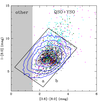
Figure 3.— $[3.6]-[8.0]$/$\hbox{I}-[8.0]$ color-color distributions. The smoothed contours show the distribution of AGN wedge objects in the SDWFS extragalactic survey (2, 5, 10, 20 and 30 objects per $0.1\times 0.2$ mag color bin). The gray shaded region corresponds to the “other” region of Cut #2. The black, red, dark green and orange points show our QSO-A, QSO-B, YSO-A and YSO-B candidates from the SAGE survey, while the magenta and cyan points mark the confirmed and high probability YSOs from Whitney et al. (2008). The box defines our Cut #3 dividing the color space into regions a and b.

Figure 4.— The spatial distributions of the candidate classes. While the QSO-A sources are very uniformly distributed, there are signs of inhomogeneities and small scale clustering for the more contaminated YSO-A candidates. The QSO-B sources have a fairly uniform distribution and there are too few YSO-B objects to draw any conclusions.

4. Summary and Conclusions

We present a simple modification of the extragalactic mid-IR quasar selection method of Stern et al. (2005) for use in dense stellar fields. Only the relatively rare, dusty stars are a source of contamination. Of such stars, AGB stars are relatively easily eliminated while sources like YSOs and dusty PNe are significant contaminants when searching for the rarer bright quasars or near the color locus of black bodies. We derive catalogs of 4,699 and 657 quasar candidates for the LMC and SMC using the SAGE (Meixner et al. 2006) and S3MC (Bolatto et al. 2007) surveys, respectively. We recover close to 100% of the known quasars in the SAGE/S3MC survey regions, demonstrating the efficiency of our selection method. The purity of our sample compared to a similar extragalactic search will be very high in the primary QSO-A region, poorer if searching for the brightest quasars in the YSO-A region, and very poor in the QSO/YSO-B regions where the color locus of black bodies crosses the Stern et al. (2005) color selection region. Fortunately, this region of color space contains only 10% of Böotes candidates. We have not addressed contamination by other extragalactic sources, as we know from our use of this approach in the Böotes field of the NDWFS (Stern et al. 2005, Gorjian et al. 2008) that it is quite low. In AGES, 69% (84%) of AGN wedge targets have $z>1$ ($z>0.5$) and 86% of the spectra are classed as broad-line AGN with only 1% contamination by stars.

We examined the GLIMPSE survey (Churchwell et al. 2009) of the Galactic plane as well. It is clear our approach will work, but the GLIMPSE survey depth is markedly lower than those of the Clouds, so the numbers of candidates are small. Moreover, the survey is largely confined to regions of very high visual extinction where spectroscopic confirmation is infeasible. Note, however, that the problem of stellar contamination diminishes in the Galactic plane relative to the Clouds because the dusty stars are shifted to lower apparent magnitudes, moving them away from the quasars. In lower stellar density fields, like those of dwarf spheroidals; it would be straightforward to use variants of our approach based on only the $[3.6]$ and $[4.5]$ bands to efficiently identify background quasars with warm Spitzer.

Follow-up spectroscopy with AAOmega on the Anglo-Australian telescope (e.g., Colless et al. 2001) could efficiently confirm the candidates, since its large field of view and fiber number are well-matched to the source density. With an expansion in the number of extragalactic reference sources by well over an order of magnitude, future improvements in the proper motions of the Clouds will be limited by the time needed to make the proper motion measurements rather than by the availability of reference sources. Finding quasars for absorption line studies will require working in the higher contamination YSO region of our selection method.

Perhaps most importantly, these are the most intensively monitored quasars we presently have. Many will have well-sampled light curves extending for over a decade, allowing large statistical studies of the variability properties of individual quasars rather than ensembles of quasars. Spectroscopy serves not only to determine the redshift but also to supply an estimate of the quasar black hole masses based on their emission line widths (e.g., Kaspi et al. 2000). With large samples it will quickly become clear if the tantalizing correlations between variability properties and intrinsic properties noted by Kelly et al. (2009) hold generally.

Table 1AGN Candidates Behind the Large Magellanic Cloud

SAGE ID	RA	Dec	[3.6]	$\sigma$[3.6]	[4.5]	$\sigma$[4.5]	[5.8]	$\sigma$[5.8]	[8.0]	$\sigma$[8.0]	V	$\sigma$V	I	$\sigma$I	OGLE-III ID	type	z	Ref.
J042911.59-701649.5	67.29833	$-$70.28043	15.54	0.06	14.82	0.11	13.98	0.08	13.01	0.06	99.99	9.99	20.77	0.27	lmc158.6.1570	QSO-Aa	-1	-1
J043014.94-701457.9	67.56225	$-$70.24942	16.09	0.09	15.26	0.12	14.33	0.14	13.02	0.09	20.57	0.11	19.76	0.13	lmc158.5.2597	QSO-Aa	-1	-1
J043025.71-690419.1	67.60714	$-$69.07199	15.98	0.05	15.35	0.08	14.48	0.11	13.60	0.08	21.40	0.16	20.31	0.21	lmc156.5.1120	QSO-Aa	-1	-1
J043036.29-690727.5	67.65124	$-$69.12432	14.71	0.04	13.94	0.06	13.10	0.05	12.14	0.04	20.36	0.13	19.04	0.13	lmc156.6.398	QSO-Aa	-1	-1
J043036.81-702131.2	67.65339	$-$70.35866	15.51	0.07	14.69	0.07	13.73	0.10	12.72	0.05	20.99	0.21	19.79	0.16	lmc158.6.2269	QSO-Aa	-1	-1

Note. — The “Type” column gives the candidates’ selection flags QSO/YSO-[AB][0ab] where $0$ for Cut 3 means that the source had no optical match because it was either outside the OGLE-III regions or too faint. We also indicate if the source is a known quasar (redshift and reference), if it is flagged as a YSO by Whitney et al. (2008), and if it is within the 90% confidence radius of a ROSAT source (HP99, Haberl & Pietsch 1999). We estimate that 30% of the ROSAT identifications will be false positives. For the ROSAT sources we indicate the ROSAT catalog number using the format HP99_number. Unmeasured magnitudes and errors are indicated by 99.999 and 9.999 respectively. One RA, Dec and magnitude digit has been truncated in this illustrative table in order to fit the page.

Table 2AGN Candidates Behind the Small Magellanic Cloud

S3MC ID	RA	Dec	[3.6]	$\sigma$[3.6]	[4.5]	$\sigma$[4.5]	[5.8]	$\sigma$[5.8]	[8.0]	$\sigma$[8.0]	V	$\sigma$V	I	$\sigma$I	OGLE-III ID	type	z	Ref.
J004255.06-732306.18	10.72944	$-$73.38505	15.62	0.02	15.00	0.01	14.02	0.04	13.21	0.06	20.39	0.26	19.61	0.34	smc125.2.30297	QSO-Aa	-1	-1
J004255.51-732309.03	10.73132	$-$73.38584	15.46	0.02	14.87	0.01	13.81	0.03	12.81	0.05	20.39	0.23	19.33	0.16	smc125.2.30304	QSO-Aa	-1	-1
J004258.33-732407.37	10.74308	$-$73.40205	15.68	0.02	15.14	0.02	13.69	0.03	12.52	0.03	19.82	0.06	19.28	0.10	smc125.2.30349	QSO-Aa	-1	-1
J004323.89-732043.39	10.84956	$-$73.34539	17.34	0.07	16.94	0.08	15.47	0.11	14.57	0.16	20.92	0.13	20.95	0.35	smc125.2.41237	QSO-Aa	-1	-1
J004413.65-724302.23	11.05690	$-$72.71729	16.15	0.03	15.34	0.02	14.12	0.04	13.16	0.05	21.42	0.36	20.23	0.25	smc126.3.9008	QSO-Aa	-1	-1

Note. — We indicate if the source is a known quasar (redshift and reference), if it is flagged as a YSO by Bolatto et al. (2007), and if it is within the 90% confidence radius of a ROSAT source (H00, Haberl et al. 2000). For the ROSAT sources we indicate the ROSAT catalog number using format H00_number. Unmeasured magnitudes and errors are indicated by 99.999 and 9.999 respectively. One RA, Dec and magnitude digit has been truncated in this illustrative table in order to fit the page.

References

- Afonso et al. (1999) Afonso, C., et al. 1999, A&A, 344, 63L
- Alcock et al. (2000) Alcock, C., et al. 2000, ApJ, 542, 281
- Anguita et al. (2000) Anguita, C., Loyola, P. & Pedreros, M. H., 2000, AJ, 120, 845
- Ashby et al. (2009) Ashby, M. L. N., et al. 2009, ApJ, 701, 428
- Blum et al. (2006) Blum, R. D., et al. 2006, AJ, 132, 2034
- Bolatto et al. (2007) Bolatto, A. D., et al. 2007, ApJ, 655, 212
- Bond et al. (2001) Bond, I A., et al. 2001, MNRAS, 327, 868
- Bramich et al. (2008) Bramich, D. M., et al. 2008, MNRAS, 386, 887
- Churchwell et al. (2009) Churchwell, E., et al. 2009, PASP, 121, 213
- Clarkson et al. (2008) Clarkson, W., et al. 2008, ApJ, 684, 1110
- Colless et al. (2001) Colless, M., et al. 2001, MNRAS, 328, 1039
- de Vries et al. (2003) de Vries, W. H., Becker, R. H., & White, R. L. 2003, AJ, 126, 1217
- Dobrzycki et al. (2002) Dobrzycki, A., Groot, P. J., Macri, L. M., Stanek, K. Z. 2002, ApJ, 569, 15
- Dobrzycki et al. (2005) Dobrzycki, A., Eyer, L., Stanek, K. Z., & Macri, L. M. 2005, A&A, 442, 495
- Drake et al. (2001) Drake, A. J. 2001, BAAS, 33, 1379
- Eisenhardt et al. (2004) Eisenhardt, P. R., et al. 2004, ApJS, 154, 48
- Eyer (2002) Eyer, L. 2002, Acta Astron,, 52, 241
- Filipovic et al. (1998) Filipovic, M. D., et al. 1998, A&AS, 127, 119
- Geha et al. (2003) Geha, M., et al. 2003, AJ, 125, 1
- Gorjian et al. (2008) Gorjian, V., et al. 2008, ApJ, 679, 1040
- Haberl & Pietsch (1999) Haberl, F., Pietsch, W. 1999, A&AS, 139, 277
- Haberl et al. (2000) Haberl, F., Filipovic, M. D., Pietsch, W., Kahabka, P. 2000, A&AS, 142, 41
- Jackson et al. (2002) Jackson, C. A., Wall, J. V., Shaver, P. A., Kellermann, K. I., Hook, I. M., & Hawkins, M. R. S. 2002, A&A, 386, 97
- Jannuzi & Dey (1999) Jannuzi, B. T., & Dey, A. 1999, in ASP Conf. Ser. 191, 111
- Jones et al. (1994) Jones, B.F., Kemola, A.R., & Lin, D.N.C. 1994, AJ, 107, 1333
- Kallivayalil et al. (2006a) Kallivayalil, N., et al. 2006, ApJ, 638, 772
- Kallivayalil et al. (2006b) Kallivayalil, N., van der Marel, R. P., & Alcock, C. 2006, ApJ, 652, 1213
- Kaspi et al. (2000) Kaspi, S., Smith, P. S., Netzer, H., Maoz, D., Jannuzi, B. T.; Giveon, U. 2000, ApJ, 533, 631
- Kelly et al. (2009) Kelly, B. C., Bechtold, J., & Siemiginowska, A. 2009, ApJ, 698, 895
- Kim et al. (1998) Kim, S., Staveley-Smith, L., Dopita, M. A., Freeman, K. C., Sault, R. J., Kesteven, M. J., McConnell, D. 1998, ApJ, 503, 674
- Kozłowski et al. (2006) Kozłowski, S., Woźniak, P. R., Mao, S., Smith, M. C., Sumi, T., Vestrand, W. T., & Wyrzykowski, Ł. 2006, MNRAS, 370, 435
- Kuijken & Rich (2002) Kuijken, K., & Rich, R. M., 2002 AJ, 124, 2054
- Lacy et al. (2004) Lacy, M., et al., 2004 ApJS, 124, 166
- Lehner et al. (2008) Lehner, N., Howk, J. C., Keenan, F. P., Smoker, J. V. 2008, ApJ, 678, 219L
- Meixner et al. (2006) Meixner, M., et al. 2006, AJ, 132, 2268
- Misawa et al. (2009) Misawa, T., Charlton, J. C., Kobulnicky, H. A., Wakker, B. P., & Bland-Hawthorn, J. 2009, arXiv:0902.0208
- Pedreros et al. (2002) Pedreros, M. H., Anguita, C., & Maza, J. 2002, AJ, 123, 1971
- Pedreros et al. (2006) Pedreros, M. H., Costa, E., Mendez, R. A. 2006, AJ, 131, 1461
- Pejcha & Stanek (2009) Pejcha, O., & Stanek, K. Z. 2009, ApJ, submitted (arXiv:0905.3389)
- Piatek et al. (2008) Piatek, S., Pryor, C., & Olszewski, E. W. 2008, AJ, 135, 1024
- Rattenbury et al. (2007) Rattenbury, N. J., Mao, S., Debattista, V. P., Sumi, T., Gerhard, O., & de Lorenzi, F. 2007, MNRAS, 378, 1165
- Richards et al. (2009) Richards, G. T., et al. 2009, ApJS, 180, 67
- Ringstorf et al. (2009) Ringstorf, A.W., et al. 2009, ApJS, 181, 129
- Savage (1976) Savage, A., 1976 MNRAS, 174, 259
- Savage et al. (2000) Savage, B. D., et al. 2000, ApJS, 129, 563
- Sembach et al. (2000) Sembach, K. R., et al. 2000, ApJ, 538, 31L
- Shull et al. (2000) Shull, J. M., et al. 2000, ApJ, 538, 73L
- Smoker et al. (2005) Smoker, J. V., Keenan, F. P., Thompson, H. M. A., Brüns, C., Muller, E., Lehner, N., Lee, J.-K., & Hunter, I. 2005, A&A, 443, 525
- Spaenhauer et al. (1992) Spaenhauer, A., Jones, B. F., & Whitford, A. E. 1992, AJ, 103, 297
- Stern et al. (2005) Stern, D., et at. 2005, ApJ, 631, 163
- Sumi et al. (2005) Sumi T., et al. 2005, MNRAS, 356, 331
- Tinney et al. (1997) Tinney, C. G., Da Costa, G. S., & Zinnecker, H. 1997, MNRAS, 285, 111
- Udalski (2003) Udalski, A. 2003, Acta Astron., 53, 291
- Udalski et al. (2008a) Udalski A., Szymański M. K., Soszyński I., Poleski R. 2008, Acta Astron., 58, 69
- Udalski et al. (2008b) Udalski, A., et al. 2008, Acta Astron., 58, 89
- Udalski et al. (2008c) Udalski, A., et al. 2008, Acta Astron., 58, 329
- Vanden Berk et al. (2004) Vanden Berk, D. E., et al. 2004, ApJ, 601, 692
- Vieira et al. (2007) Vieira, K., et al. 2007, AJ, 134, 1432
- Whitney et al. (2008) Whitney, B. A., et al. 2008, AJ, 136, 18