Regime Switching Stochastic Volatility with Perturbation Based Option Pricing
by
Sovan Mitra

Abstract

Volatility modelling has become a significant area of research within Financial Mathematics. Wiener process driven stochastic volatility models have become popular due their consistency with theoretical arguments and empirical observations. However such models lack the ability to take into account long term and fundamental economic factors e.g. credit crunch.

Regime switching models with mean reverting stochastic volatility are a new class of stochastic volatility models that capture both short and long term characteristics. We propose a new general method of pricing options for these new class of stochastic volatility models using Fouque’s perturbation based option pricing method.

Using empirical data, we compare our option pricing method to Black-Scholes and Fouque’s standard option pricing method and show that our pricing method provides lower relative error compared to the other two methods.

Key words: Stochastic volatility, option pricing, perturbation theory.

1 Introduction and Outline

Volatility modelling has become a significant area of research within Financial Mathematics: it helps us understand price dynamics since it is one of the key variables in a stochastic differential equation. Volatility is the only variable in the Black-Scholes option pricing equation that is unobservable, hence crucial to option pricing. Finally, volatility has a wide range of industrial applications from pricing exotic derivatives to asset pricing models [41]. Shiller [44] also claims volatility can be used as a measure of market efficiency.

With volatility modelling, stochastic volatility has achieved growing importance as they capture a richer set of empirical and theoretical characteristics compared to other volatility models [38]:

• firstly, stochastic volatility models generate return distributions similar to what is empirically observed. For example, the return distribution has a fatter left tail and peakedness compared to normal distributions, with tail asymmetry controlled by $\rho$ [12].

• Secondly, Renault and Touzi [42] proved volatility that is stochastic and $\rho$=0 always produces implied volatilities that smile (note that volatility smiles do not necessarily imply volatility is stochastic).

• Thirdly, historic volatility shows significantly higher variability than would be expected from local or time dependent volatility, which could be better explained by a stochastic process. A particular case in point is the dramatic change in volatility during the 1987 October crash (Schwert [46] gives an empirical study on this). Finally, stochastic volatility accounts for the volatility’s empirical dependence on the time scale measured, which should not occur under local or time dependent volatility.

Wiener process driven stochastic volatility models capture price and volatility dynamics more successfully compared to local and time dependent volatility models. However, for longer term dynamics and fundamental economic changes (e.g. “credit crunch”), no mechanism existed to address the change in volatility dynamics and it has been empirically shown that volatility is related to long term and fundamental conditions. To model volatility (and stock prices) in continuous time but also capture long term and fundamental factors requires regime switching models with mean reverting stochastic volatility. This is a currently growing area of stochastic volatility models.

At present, there is no method for pricing options for volatility governed by regime switching with mean reverting stochastic volatility. Using Fouque’s [17] perturbation approach to stochastic volatility option pricing, we show how it is possible to obtain option prices. Additionally, the option pricing method is possible for any mean reverting process. We demonstrate our method with empirical results from S&P 500 index options.

The outline of the paper is as follows. Firstly we give a literature review of volatility models and the option pricing methods. We then explain Fouque’s option pricing method under standard mean reverting stochastic volatility and then show how it can be applied to regime switching with meaning reverting stochastic volatility. We finally provide numerical experiments, demonstrating that our method of option pricing provides more accurate prices compared to standard Fouque option pricing (without regimes).

2 Literature Review on Volatility Models

Bachelier [3] proposed the first model for stock prices. Bachelier reasoned that investing was theoretically a “fair game” in the sense that statistically one could neither profit nor lose from it. Hence Bachelier included the Wiener process to incorporate the random nature of stock prices. Osborne [39] conducted empirical work supporting Bachelier’s model. Samuelson [43] continued the constant volatility model under the Geometric Brownian Motion stock price model on the basis of economic justifications.

Over time, empirical data and theoretical arguments found constant volatility to be inconsistent with the observed market behaviour (such as the leverage effect). A plot of the empirical daily volatility of the S&P 500 index clearly shows volatility is far from constant. This consequently led to the development of dynamic volatility modelling, which we will now discuss.

2.1 Time Dependent Volatility Model

It was empirically observed that implied volatility varied with an option’s expiration date. Consequently, a straight forward extension proposed to the constant volatility model was time dependent volatility modelling [57]:

$$dX/X=\mu dt+\sigma(t)dW.$$ (1)

Merton [35] was the first to propose a formula for pricing options under time dependent volatility. The option price associated with X is still calculated by the standard Black-Scholes formula except we set $\sigma={\sigma}_{c}$ where:

$$\sigma_{c}=\sqrt{\dfrac{1}{T-t}\int^{T}_{t}\sigma^{2}(\tau)d\tau},$$ (2)

i.e. $d_{1}$ and $d_{2}$ in the Black-Scholes equation become:

$$d_{1} = \dfrac{log\left(\dfrac{X}{K}\right)+\mu(T-t)+\dfrac{1}{2}\int^{T}_{t}\sigma^{2}(\tau)d\tau}{\sqrt{\int^{T}_{t}\sigma^{2}(\tau)d\tau}},$$ (3)

$$d_{2} = \dfrac{log\left(\dfrac{X}{K}\right)+\mu(T-t)-\dfrac{1}{2}\int^{T}_{t}\sigma^{2}(\tau)d\tau}{\sqrt{\int^{T}_{t}\sigma^{2}(\tau)d\tau}}.$$ (4)

The equation (2) converts $\sigma(t)$ to its constant volatility equivalent $\sigma_{c}$ over time period t to T. The distribution of X(t) is given by:

$$log(X_{T}/X_{t})\sim\mathcal{N}\left((\mu-\frac{1}{2}\sigma_{c}^{2})(T-t),\sigma_{c}^{2}(T-t)\right).$$ (5)

Note that the constant volatility $\sigma_{c}$ changes in value as t and T change. This property enables time dependent volatility to account for empirically observed implied volatilities increasing with time (for a given strike).

2.2 Local Volatility Model: Definition and Characteristics

In explaining the empirical characteristics of volatility, a time dependent volatility model was found to be insufficient. For instance, time dependent volatility did not explain the volatility smile, nor the leverage effect, since volatility cannot vary with price. Therefore volatility as a function of price (and optionally time) was proposed, that is local volatility is $\sigma=f(X,t)$:

$$dX/X=\mu dt+\sigma(X,t)dW.$$ (6)

The term “local” arises from knowing volatility with certainty “locally” or when X is known -for a stochastic volatility model we never know the volatility with certainty.

The advantages of local volatility models are that firstly, no additional (or untradable) source of randomness is introduced into the model. Hence the models are complete, unlike stochastic volatility models. It is theoretically possible to perfectly hedge contingent claims. Secondly, local volatility models can be also calibrated to perfectly fit empirically observed implied volatility surfaces, enabling consistent pricing of the derivatives (an example is given in [11]). Thirdly, the local volatility model is able to account for a greater degree of empirical observations and theoretical arguments on volatility than time dependent volatility (for instance the leverage effect).

Some common local volatility models are: the Constant Elasticity of Variance Model (CEV) proposed by Cox and Ross [7], Mixture Distribution Models by Brigo and Mercurio [5] and the Implied Local Volatility by Dupire [10], Derman and Kani [8].

2.3 Stochastic Volatility Model: Definition and Characteristics

Although local volatility models were an improvement on time dependent volatility, they possessed certain undesirable properties. For example, volatility is perfectly correlated (positively or negatively) with stock price yet empirical observations suggest no perfect correlation exists. Stock prices empirically exhibit volatility clustering but under local volatility this does not necessarily occur. Consequently after local volatility development, models were proposed that allowed volatility to be governed by its own stochastic process. We now define stochastic volatility.

Definition 1.

Assume X follows the stochastic differential equation

$$dX/X = \mu dt+\sigma(\omega)dW_{1}.$$ (7)

Volatility is stochastic if $\sigma(\omega)$ is governed by a stochastic process that is driven by another (but possibly correlated) random process, typically another Wiener process $dW_{2}$. The probability space $(\Omega,\mathcal{F},\mathbb{P})$ is $\Omega=\mathcal{C}([0,\infty):\mathbb{R}^{2})$, with filtration $\{\mathcal{F}_{t}\}_{t\geq 0}$ representing information on two Wiener processes $(W_{1},W_{2})$.
The process governing $\sigma(\omega)$ must always be positive for all values since volatility can only be positive. The Wiener processes have instantaneous correlation $\rho$ $\in[-1,1]$ defined by:

$$corr(dW_{1}(t),dW_{2}(t))=\rho dt.$$

Empirically $\rho$ tends to be negative in equity markets due to the leverage effect but close to 0 in the currency markets. Significant stochastic volatility models include: Johnson and Shanno [27], Scott Model [47], Hull-White Model [26], Stein and Stein Model [51], Heston model [22]

The key difference between local and stochastic volatility is that local volatility is not driven by a random process of its own; there exists only one source of randomness ($dW_{1}$). In stochastic volatility models, volatility has its own source of randomness ($dW_{2}$) making volatility intrinsically stochastic. We can therefore never definitely determine the volatility’s value, unlike in local volatility.

The disadvantages of stochastic volatility are firstly that these models introduce a non-tradable source of randomness, hence the market is no longer complete and we can no longer uniquely price options or perfectly hedge. Therefore the practical applications of stochastic volatility are limited. Secondly stochastic volatility models tend to be analytically less tractable. In fact, it is common for stochastic volatility models to have no closed form solutions for option prices. Consequently option prices can only be calculated by simulation.

Stochastic volatility models fundamentally differ according to their driving mechanisms for their volatility process. Different driving mechanisms maybe favoured due to their tractability, theoretical or empirical appeal and we can categorise stochastic volatility models according to them. Many stochastic volatility models favour a mean reverting driving process. A mean reverting stochastic volatility process is of the form [17]:

$$\sigma = f(Y),$$ (8)

$$dY = \alpha(m-Y)dt+\beta dW_{2},$$ (9)

where:

• $\beta\geq 0$ and $\beta$ is a constant;

• m is the long run mean value of $\sigma$;

• $\alpha$ is the rate of mean reversion.

Mean reversion is the tendency for a process to revert around its long run mean value. We can economically account for the existence of mean reversion through the cobweb theorem, which claims prices mean revert due to lags in supply and demand [33]. The inclusion of mean reversion ($\alpha$) within volatility is important, in particular, it controls the degree of volatility clustering (burstiness) if all other parameters are unchanged. Volatility clustering is an important empirical characteristic of many economic or financial time series [15], which neither local nor time dependent volatility models necessarily capture. Additionally, a high $\frac{1}{\alpha}$ can be thought of as the time required to decorrelate or “forget” its previous value.

The equation (9) is an Ornstein-Uhlenbeck process in Y. It is known the solution to equation (9) is:

$$Y(t)=m+(Y(0)-m)e^{-\alpha t}+\beta\int^{t}_{0}e^{-\alpha t}dW_{2},$$ (10)

where Y(t) has the distribution

$$Y(t)\sim\mathcal{N}\left(m+(Y(0)-m)e^{-\alpha t},\frac{\beta^{2}}{2\alpha}(1-e^{-2\alpha t})\right).$$ (11)

Note that alternative processes to equation (9) could have been proposed to define volatility as a mean reverting stochastic volatility model, for example the Feller or Cox-Ingersoll-Ross (CIR) process [18]:

$$dY = \alpha(m-Y)dt+\beta\sqrt{Y}dW_{2}.$$ (12)

However with $\sigma=f(Y)$ in equation (9) we can represent a broad range of mean reverting stochastic volatility models in terms of a function of Y.

2.4 Regime Switching Volatility

2.4.1 General Regime Switching

A class of models that address fundamental and long term volatility modelling is the regime switching model (or hidden Markov model) e.g. as discussed in [54],[16]. In fact, Schwert suggests in [45] that volatility changes during the Great Depression can be accounted for by a regime change such as in Hamilton’s regime switching model [20]. For regime switching models, generally the return distribution rather than the continuous time process is specified. A typical example of a regime switching model is Hardy’s model [21]:

$$log((X(t+1)/X(t))|i)\sim\mathcal{N}(u_{i},\varphi_{i}),i\in\{1,..,R\},$$ (13)

where

• $\varphi_{i}$ and $u_{i}$ are constant for the duration of the regime;

• i denotes the current regime (also called the Markov state or hidden Markov state);

• R denotes the total number of regimes;

• a transition matrix A is specified.

For Hardy’s model the regime changes discretely in monthly time steps but stochastically, according to a Markov process.

Due to the ability of regime switching models to capture long term and fundamental changes, regime switching models are primarily focussed on modelling the long term behaviour, rather than the continuous time dynamics. Therefore regime switching models switch regimes over time periods of months, rather than switching in continuous time. Examples of regime switching models that model dynamics over shorter time periods are Valls-Pereira et al.[56], who propose a regime switching GARCH process, while Hamilton and Susmel [25] give a regime switching ARCH process. Note that economic variables other than stock returns, such as inflation, can also be modelled using regime switching models.

The theory of Markov models (MM) and Hidden Markov models (HMM) are methods of mathematically modelling time varying dynamics of certain statistical processes, requiring a weak set of assumptions yet allow us to deduce a significant number of properties. MM and HMM model a stochastic process (or any system) as a set of states with each state possessing a set of signals or observations. The models have been used in diverse applications such as economics [52], queuing theory [48], engineering [53] and biological modelling [36]. Following Taylor [55] we define a Markov model:

Definition 2.

A Markov model is a stochastic process $X(t)$ with a countable set of states and possesses the Markov property:

$$p(q_{t+1}=j\mid q_{1},q_{2},..,q_{t}=i)=p(q_{t+1}=j\mid q_{t}=i),$$ (14)

where

• $q_{t}$ is the Markov state (or regime) at time t of $X(t)$;

• i and j are specific Markov states.

As time passes the process may remain or change to another state (known as state transition). The state transition probability matrix (also known as the transition kernel or stochastic matrix) $\mathbf{A}$, with elements $a_{ij}$, tells us the probability of the process changing to state j given that we are now in state i, that is $a_{ij}=p(q_{t+1}=j\mid q_{t}=i)$. Note that $a_{ij}$ is subject to the standard probability constraints:

$$0\leq a_{ij} \leq 1,\forall i,j,$$ (15)

$$\sum^{\infty}_{j=1}a_{ij} = 1,\forall i.$$ (16)

We assume that all probabilities are stationary in time. From the definition of a MM the following proposition follows:

Proposition 1.

A Markov model is completely defined once the following parameters are known:

• R, the total number of regimes or (hidden) states;

• state transition probability matrix $\mathbf{A}$ of size $R\times R$. Each element is $a_{ij}=p(q_{t+1}=j|q_{t}=i)$, where i refers to the matrix row number and j to the column number of $\mathbf{A}$;

• initial (t=1) state probabilities $\pi_{i}=p(q_{1}=i),\forall i$.

A hidden Markov model is simply a Markov model where we assume (as a modeller) we do not observe the Markov states. Instead of observing the Markov states (as in standard Markov models) we detect observations or time series data where each observation is assumed to be a function of the hidden Markov state, thus enabling statistical inferences about the HMM. Note that in a HMM it is the states which must be governed by a Markov process, not the observations and throughout we will assume one observation occurs after one state transition.

Proposition 2.

A hidden Markov model is fully defined when the parameter set $\{\mathbf{A},\mathbf{B},\mathbf{\pi}\}$ are known:

• R, the total number of (hidden) states or regimes;

• A, the (hidden) state transition matrix of size $R\times R$. Each element is $a_{ij}=p(q_{t+1}=j|q_{t}=i)$;

• initial (t=1) state probabilities $\pi_{i}=p(q_{1}=i),\forall i$;

• B, the observation matrix, where each entry is $b_{j}(O_{t})=p(O_{t}|j)$ for observation $O_{t}$. For $b_{j}(O_{t})$ is typically defined to follow some continuous distribution e.g. $b_{j}(O_{t})\sim\mathcal{N}(u_{j},\varphi_{j})$.

Regime switching has been developed by various researchers. For example, Kim and Yoo [31] develop a multivariate regime switching model for coincident economic indicators. Honda [24] determines the optimal portfolio choice in terms of utility for assets following GBM but with continuous time regime switching mean returns. Alexander and Kaeck [1] apply regime switching to credit default swap spreads, Durland and McCurdy [9] propose a model with a transition matrix that specifies state durations.

2.4.2 Regime Switching Mean Reverting Stochastic Volatility Models

A common shortfall in all the volatility models reviewed so far has been that all these models are short or long term volatility models. The models implicitly ignore any long term or broader economic factors influencing the volatility model, which is empirically unrealistic and theoretically inconsistent.

Combining Wiener process driven stochastic volatility models with regime switching would give the benefits of capturing the short term price dynamics while the regime switching would capture volatility changes due to fundamental and longer term effects in a tractable method. In fact Alexander combines two models to model short and long term dynamics, giving the binomial mixture distribution model [2] (mixture distribution model and a binomial tree).

A model that addresses both the long and short term dynamics are regime switching mean reverting volatility models (RSMR). These RSMR models are of the form where the intra-regime (within regime) dynamics follow an exponential Ornstein-Uhlenbeck process (expOU):

$$dX/X = \mu_{i}dt+\sigma_{i}^{\prime}(\omega)dW_{1},$$ (17)

$$d\sigma_{i}^{\prime}/\sigma_{i}^{\prime} = \left[\alpha_{i}^{\prime}(m_{i}^{\prime}-ln\sigma_{i}^{\prime})+\dfrac{{\beta^{\prime}}_{i}^{2}}{2}\right]dt+\beta_{i}^{\prime}dW_{2},$$ (18)

$$i \in \{1,2\}.$$ (19)

Alternatively, it can be more convenient to express RSexpOU in terms of OU:

$$dX/X = \mu_{i}dt+\sigma_{i}(\omega)dW_{1},$$ (20)

$$\sigma_{i} = exp(Y_{i}(t)),$$ (21)

$$dY_{i}(t) = \alpha_{i}(m_{i}-Y_{i})dt+\beta_{i}dW_{2}.$$ (22)

We denote i as the current regime and for convenience set R=2. The regime switching process is a discrete time Markov process (e.g. changing in time intervals of one year).We note that regime switching models that change state continuously do not capture long term and sustained changes. In fact Hamilton’s regime switching models have discrete time switching periods of three months (see for instance [14]).

The literature on regime switching models with stochastic differential equations in their continuous time price dynamics is currently growing but is not significant, especially for mean reverting stochastic volatility. Examples include Kalimipalli [30] and Smith [50], who describe a stochastic volatility model with regime switching to model interest rates, Elliot et al. [13] propose a regime switching Geometric Brownian Motion model (GBM) and Mari [34] models electricity spot prices with each regime possessing a different stochastic differential equation structure, such as mean reversion in the drift.

3 Perturbation Based Option Pricing

We price options for RSMR model using Fouque’s option pricing method, which is based on perturbation theory. Fouque’s perturbation method is normally applied to mean reverting stochastic volatility models; we briefly introduce Fouque’s perturbation theory by first introducing perturbation analysis and then Fouque’s method. Finally we show we can apply Fouque’s method to RSMR models. For more information on perturbation theory the reader is referred to Hinch [23], Simmonds [49], Bender and Orszag [6].

3.1 Introduction to Perturbation Analysis

For many mathematical equations we cannot find precise solutions, however, we would like to obtain approximations in a mathematically consistent and rigorous way. The perturbation method is applied when we know the solution to an equation but would like to know the solutions when variables are minutely changed (or perturbed) by a small amount $\epsilon$, where $\epsilon\rightarrow 0$ but is finite. Perturbation problems can be solved by an iterative method or by a series expansion method; Fouque adopts the latter method.

Perturbation analysis can be explained by example; consider the following example equation we wish to solve:

$$x^{2}-1=x.$$ (23)

This equation can be easily solved using knowledge of quadratics. Now consider when we perturb this problem by $\epsilon$:

$$x^{2}-1=\epsilon x,\mbox{where }\epsilon\rightarrow 0.$$ (24)

Solving for x now becomes difficult for various small (but finite) values of $\epsilon$. Note that in this example it is still possible to find the 2 analytic solutions to equation (24) using our knowledge of quadratics:

$$x_{a} = \epsilon/2+\sqrt{(1+\epsilon^{2})/4},$$ (25)

$$x_{b} = \epsilon/2-\sqrt{(1+\epsilon^{2})/4}.$$ (26)

However, instead of using knowledge of quadratics we apply the perturbation method: we determine the solutions $x_{a},x_{b}$ by approximating x by a series expansion. One could use any series expansion (e.g. Taylor, Maclaurin) but we use a power series expansion:

$$x = \sum_{n=0}^{\infty}x_{n}\epsilon^{n}$$ (27)

$$= x_{0}+\epsilon x_{1}+\epsilon^{2}x_{2}+\epsilon^{3}x_{3}+....$$ (28)

where $x_{1},x_{2},x_{3}$ are constants to be determined. Note that $x_{0}$ is called the leading term, $x_{1}$ the first correction, $x_{2}$ the second correction and so on. The unperturbed or known solution corresponds to $\epsilon=0$ and therefore equals $x_{0}$. Normally obtaining a solution to the unperturbed problem (that is $x_{0}$) is easy to obtain, otherwise the set of equations (as shown later) that need to be solved to obtain approximations to $x_{a},x_{b}$ will be difficult to solve.

With the series approximation of x (equation (28)), we insert this approximation into the original equation (24):

$$x^{2}-1 = \epsilon x$$

$$(x_{0}+\epsilon x_{1}+\epsilon^{2}x_{2}+\epsilon^{3}x_{3})^{2}-1 = \epsilon(x_{0}+\epsilon x_{1}+\epsilon^{2}x_{2}+\epsilon^{3}x_{3})$$

$$(x_{0}^{2}+2\epsilon x_{0}x_{1}+\epsilon^{2}(x_{1}^{2}+2x_{0}x_{2})+\mathcal{O}(\epsilon^{3})+\mathcal{O}(\epsilon^{4}))-1 = \epsilon(x_{0}+\epsilon x_{1}+\mathcal{O}(\epsilon^{3})).$$

Now it is standard practice to ignore terms of order $\epsilon^{3}$ (denoted $\mathcal{O}(\epsilon^{3})$) and higher since $\epsilon$ is small and so terms of $\mathcal{O}(\epsilon^{3})$ or higher are considered insignificant. Therefore the equation simplifies to

$$x_{0}^{2}+2\epsilon x_{0}x_{1}+\epsilon^{2}(x_{1}^{2}+2x_{0}x_{2})-1 = \epsilon x_{0}+\epsilon^{2}x_{1}$$ (29)

$$(x_{0}^{2}-1)+\epsilon(2x_{0}x_{1}-x_{0})+\epsilon^{2}(x_{1}^{2}+2x_{0}x_{2}-x_{1}) = 0.$$ (30)

Now equation (30) is significant because the bracketed terms represent coefficients of $\epsilon$ for each power and each bracketed term separately must equal 0 for the equation to balance. So now we can equate terms of the same order from equation (30):

$$\mathcal{O}(\epsilon^{0}) : x_{0}^{2}-1=0,$$ (31)

$$\mathcal{O}(\epsilon^{1}) : 2x_{0}x_{1}-x_{0}=0,$$ (32)

$$\mathcal{O}(\epsilon^{2}) : x_{1}^{2}+2x_{0}x_{2}-x_{1}=0.$$ (33)

Solving the equations (31)-(33) and remembering there are 2 solutions gives:

$$x_{a} : \{x_{0}=1,x_{1}=1/2,x_{2}=1/8\},$$ (34)

$$x_{b} : \{x_{0}=-1,x_{1}=1/2,x_{2}=-1/8\}.$$ (35)

Using these values, we can now calculate approximate but extremely accurate solutions to $x_{a},x_{b}$:

$$x = x_{0}+\epsilon x_{1}+\epsilon^{2}x_{2}+....$$ (36)

$$x_{a} = 1+\epsilon(1/2)+\epsilon^{2}(1/8)$$ (37)

$$x_{b} = -1+\epsilon(1/2)+\epsilon^{2}(-1/8).$$ (38)

To summarise, the three steps of perturbative analysis (by Bender and Orszag [6]) are: firstly to convert the original (unperturbed) problem into a perturbed problem by introducing $\epsilon$. Secondly, we assume the expression for the solution is in the form of a perturbation series and determine the coefficients of that series. Thirdly, we determine answers to the solutions by summing the perturbation series for the appropriate values of $\epsilon$.

Perturbation problems can be divided into two categories: regular and singular perturbation problems. Singular pertubation problems have significantly different solutions as $\epsilon\rightarrow 0$ when compared to the unperturbed problem ($\epsilon=0$). If the solution changes insignificantly with $\epsilon$ then we have a regular perturbation; the perturbed solution smoothly approaches the unperturbed solution as $\epsilon\rightarrow 0$. Fouque’s perturbation based option pricing method is a singular perturbation problem.

To give an example of perturbation problems, a spinning drawing pin rotates around its vertical axis and over a short time period its horizontal distance from its vertical axis is unlikely to be significantly different from its initial position (at t=0). However over long time periods, the drawing pin will eventually come to a physical rest and its horizontal position will be appreciably different than from at t=0. Therefore over a small time period the position can be modelled as a regular perturbation problem but over long time periods it is a singular perturbation problem.

3.2 Perturbation Formulation of Option Pricing

Option pricing where the stock price process is governed by stochastic volatility can be analytically challenging. Fouque [17] finds a method of pricing options whose underlying is governed by a mean reverting stochastic volatility process by solving the option pricing partial differential equation as a singular perturbation problem. A significant benefit of Fouque’s method is that the option pricing method is model independent; it can be applied to any fast mean reverting stochastic volatility model and without explicit knowledge of the volatility dynamics. Additionally, the option pricing calibration is far more parsimonious compared to other stochastic volatility option pricing methods.

To find the option pricing partial differential equation when the underlying asset is driven by mean reverting stochastic volatility, we can use a replicating portfolio argument. Alternatively, we can determine the option pricing partial differential equation associated with an option by risk neutral valuation and apply the Feynman-Kac equation, which is the approach we take here. We abbreviate call option C(X,K,s,T,r,f(Y)) to C(s,X,Y), which is an option at time s with volatility as a function of some mean reverting stochastic volatility process (f(Y)). By risk neutral valuation C(s,X,Y) is given by:

$$C(s,X,Y)=e^{-r(T-s)}E^{\mathbb{Q}}[X(T)-K|\mathcal{F}_{s}]^{+}.$$ (39)

We recall that in a no arbitrage market under stochastic volatility there is more than one risk neutral measure $\mathbb{Q}$ (no unique $\mathbb{Q}$ measure exists). The possible $\mathbb{Q}$ measures can be parameterised by the market price of volatility risk $\gamma=\gamma(t,X,f(Y))$. Therefore $\mathbb{Q}$ measures are a function of $\gamma$, consequently the price of option C(t,X,Y) is a function of $\gamma$.

To obtain the (risk neutral) option pricing partial differential equation by the Feynman-Kac equation, we require the risk neutral process. We begin with a stock price with a mean reverting stochastic volatility process, that is:

$$dX/X = \mu dt+\sigma dW_{1},$$ (40)

$$\sigma = f(Y),$$ (41)

$$dY = \alpha(m-Y)dt+\beta dW_{2}.$$ (42)

The risk neutral process for dX/X is:

$$dX/X = rdt+\sigma dW_{1}^{\mathbb{Q}}.$$ (43)

We can re-express $dW_{2}$ as [17]:

$$dW_{2}=\rho dW_{1}+\sqrt{1-\rho^{2}}dW^{*},$$ (44)

where $W^{*}$ is a standard Wiener process independent of $W_{1}$. To change dY to its risk neutral process we require:

1. $$dW_{1}^{\mathbb{Q}} = dW_{1}+\dfrac{\mu-r}{f(Y)}dt,$$ (45)

   $$\mbox{i.e. }dW_{1} = dW_{1}^{\mathbb{Q}}-\dfrac{\mu-r}{f(Y)}dt.$$ (46)

2. $$dW^{\mathbb{Q}*} = dW^{*}+\gamma(t,X,Y)dt,$$ (47)

   $$\mbox{i.e. }dW^{*} = dW^{\mathbb{Q}*}-\gamma(t,X,Y)dt.$$ (48)

To obtain the risk neutral process of dY we substitute in equations (44)-(48) and rearrange dY; starting with substituting equation (44) for $dW_{2}$ gives

$$dY = \alpha(m-Y)dt+\beta dW_{2},$$

$$= \alpha(m-Y)dt+\beta\left[\rho dW_{1}+\sqrt{1-\rho^{2}}dW^{*}\right].$$

Substituting equation (46) for $dW_{1}$ and equation (48) for $dW^{*}$ gives:

$$dY = \alpha(m-Y)dt$$

$$+ \beta\left[\rho\left(dW_{1}^{\mathbb{Q}}-\dfrac{\mu-r}{f(Y)}dt\right)+(\sqrt{1-\rho^{2}})(dW^{\mathbb{Q}*}-\gamma(t,X,Y)dt)\right].$$

Rearranging now gives:

$$dY = \left[\alpha(m-Y)-\beta\left(\rho\dfrac{(\mu-r)}{f(Y)}+\sqrt{1-\rho^{2}}\gamma(t,X,Y)\right)\right]dt$$

$$+ \beta\left[\rho dW_{1}^{\mathbb{Q}}+\sqrt{1-\rho^{2}}dW^{\mathbb{Q}*}\right].$$

Since the risk neutral equation for dX is a two dimensional diffusion equation in $(W_{1}^{\mathbb{Q}},W^{\mathbb{Q}*})$, the associated option pricing partial differential equation for C(s,X,Y) is obtained by the application of the multidimensional version of the Feynman-Kac equation with boundary condition $C(T,x,y)$.

The Feyman-Kac equations give the option pricing partial differential equation:

$$0 = \dfrac{\partial C}{\partial s}+\dfrac{1}{2}f^{2}(y)x^{2}\dfrac{\partial^{2}C}{\partial x^{2}}+\rho\beta xf(y)\dfrac{\partial^{2}C}{\partial x\partial y}+\dfrac{\beta^{2}}{2}\dfrac{\partial^{2}C}{\partial y^{2}}+r\left(x\dfrac{\partial C}{\partial x}-C\right)$$

$$+ [\alpha(m-y)-\beta\Lambda(s,x,y)]\dfrac{\partial C}{\partial y},$$

$$\mbox{where }\Lambda(s,x,y) = \rho\dfrac{(\mu-r)}{f(y)}+\sqrt{1-\rho^{2}}\gamma(s,x,y).$$

The term $\Lambda(t,x,y)$ can be interpretted as a combination of market price of risk and market price of volatility risk. Fouque assumes that $\Lambda(s,x,y)=\Lambda(y)$, a function of y only:

$$\Lambda(y) = \rho\dfrac{(\mu-r)}{f(y)}+\sqrt{1-\rho^{2}}\gamma(y).$$ (49)

Now from our knowledge of OU processes (which is also Y(t)) we know as $t\rightarrow\infty$ the distribution becomes $\mathcal{N}(m,\frac{\beta^{2}}{2\alpha})$ (see equation (11)). If we denote the variance of this long term distribution as $v^{2}$, that is $v^{2}=\frac{\beta^{2}}{2\alpha}$, then $\beta=v\sqrt{2\alpha}$ and we can re-express the option pricing partial differential equation as:

$$0 = \dfrac{\partial C}{\partial s}+\dfrac{1}{2}f^{2}(y)x^{2}\dfrac{\partial^{2}C}{\partial x^{2}}+\rho v\sqrt{2\alpha}xf(y)\dfrac{\partial^{2}C}{\partial x\partial y}+v^{2}\alpha\dfrac{\partial^{2}C}{\partial y^{2}}+r\left(x\dfrac{\partial C}{\partial x}-C\right)$$

$$+ [\alpha(m-y)-v\sqrt{2\alpha}\Lambda(y)]\dfrac{\partial C}{\partial y}.$$

Now if we re-express $\alpha$ as $\alpha=\dfrac{1}{\epsilon}$, where $\epsilon\rightarrow 0$ is small but finite (since $\alpha\rightarrow\infty$) our equation becomes:

$$0 = \dfrac{\partial C}{\partial s}+\dfrac{1}{2}f^{2}(y)x^{2}\dfrac{\partial^{2}C}{\partial x^{2}}+\rho\dfrac{v\sqrt{2}}{\sqrt{\epsilon}}xf(y)\dfrac{\partial^{2}C}{\partial x\partial y}+\dfrac{v^{2}}{\epsilon}\dfrac{\partial^{2}C}{\partial y^{2}}+r\left(x\dfrac{\partial C}{\partial x}-C\right)$$

$$+ \left[\dfrac{(m-y)}{\epsilon}-\dfrac{v\sqrt{2}}{\sqrt{\epsilon}}\Lambda(y)\right]\dfrac{\partial C}{\partial y}.$$

We can also re-express the equation using the following operator notation for convenience:

$$\mathcal{L}_{0} = v^{2}\frac{\partial^{2}}{\partial y^{2}}+(m-y)\frac{\partial}{\partial y},$$ (50)

$$\mathcal{L}_{1} = \sqrt{2}\rho vxf(y)\frac{\partial^{2}}{\partial x\partial y}-\sqrt{2}v\Lambda(y)\frac{\partial}{\partial y},$$ (51)

$$\mathcal{L}_{2} = \frac{\partial}{\partial s}+\frac{1}{2}f^{2}(y)x^{2}\frac{\partial^{2}}{\partial x^{2}}+r\left(x\frac{\partial}{\partial x}-1{\hskip-2.5pt}\hbox{I}\right).$$ (52)

Therefore the option pricing partial differential equation is:

$$\left(\frac{1}{\epsilon}\mathcal{L}_{0}+\frac{1}{\sqrt{\epsilon}}\mathcal{L}_{1}+\mathcal{L}_{2}\right)C=0.$$ (53)

Equation (53) is a (singular) perturbation problem; we can therefore solve the option pricing partial differential equation (under mean reverting stochastic volatility) by perturbation methods. We note that:

• we sometimes express $\mathcal{L}_{2}=\mathcal{L}_{BS}(f(y))$, where $\mathcal{L}_{BS}(\cdot)$ is the Black-Scholes partial differential operator with volatility $(\cdot)$.

• the $\mathcal{L}_{0}$ operator gives a Poisson equation for Y (an OU process). Note that the popular definition of a Poisson equation is a form of Laplace equation (second order partial differential equation), however, for stochastic processes it is $\mathcal{L}_{0}$.

3.3 Perturbation Solution to Option Pricing

To determine the solution to C(s,x,y) by a perturbation approach we expand C in powers of $\sqrt{\epsilon}$

$$C=C_{0}+\sqrt{\epsilon}C_{1}+\epsilon C_{2}+\epsilon^{\frac{3}{2}}C_{3}+......$$ (54)

and insert equation (54) into equation (53):

$$0 = \left(\frac{1}{\epsilon}\mathcal{L}_{0}+\frac{1}{\sqrt{\epsilon}}\mathcal{L}_{1}+\mathcal{L}_{2}\right)(C_{0}+\sqrt{\epsilon}C_{1}+\epsilon C_{2}+\epsilon^{\frac{3}{2}}C_{3}+......)$$

$$= \frac{1}{\epsilon}\mathcal{L}_{0}C_{0}$$

$$+ \frac{1}{\sqrt{\epsilon}}(\mathcal{L}_{0}C_{1}+\mathcal{L}_{1}C_{0})$$

$$+ (\mathcal{L}_{0}C_{2}+\mathcal{L}_{1}C_{1}+\mathcal{L}_{2}C_{0})$$

$$+ \sqrt{\epsilon}(\mathcal{L}_{0}C_{3}+\mathcal{L}_{1}C_{2}+\mathcal{L}_{2}C_{1})$$

$$+ \mathcal{O}(\epsilon).$$

As with standard perturbation problems, we can equate terms of the same order to assist us in solving the equation. Fouque solves C upto $C=C_{0}+\sqrt{\epsilon}C_{1}$ (although we could solve further), therefore our aim is to find $C_{0}$ and $C_{1}$.

Zero Order Term ($C_{0}$)
We begin by firstly determining $C_{0}$; by equating terms of order $1/\epsilon$ we have:

$$\mathcal{L}_{0}C_{0}=0.$$ (55)

For equation (55) to be correct and since $\mathcal{L}_{0}$ acts only on y, $C_{0}$ must be a function of s,x only: $C_{0}=C_{0}(s,x)$.

Now equating terms of order $1/\sqrt{\epsilon}$ we have:

$$\mathcal{L}_{0}C_{1}+\mathcal{L}_{1}C_{0}=0.$$ (56)

For equation (56) to be correct, if $\mathcal{L}_{1}$ takes derivatives on y only and since we have already deduced $C_{0}=C_{0}(s,x)$ therefore we have $\mathcal{L}_{1}C_{0}=0$. This in turn implies from equation (56) that $\mathcal{L}_{0}C_{1}=0$, which in turn implies $C_{1}=C_{1}(s,x)$ for equation (56) to be correct. If desired one could continue to apply this iterative method for higher orders 1, $\epsilon$ and so on to obtain further equations.

Now the order 1 terms give:

$$\mathcal{L}_{0}C_{2}+\mathcal{L}_{1}C_{1}+\mathcal{L}_{2}C_{0}=0.$$ (57)

Since we have already reasoned $\mathcal{L}_{1}C_{1}$=0 we can write

$$\mathcal{L}_{0}C_{2}+\mathcal{L}_{2}C_{0}=0.$$ (58)

Regarding the variable x as fixed $\mathcal{L}_{2}C_{0}$ is a function of y since $\mathcal{L}_{2}$ contains f(y); if we focus on the y dependency only we can rewrite equation (58) as:

$$\mathcal{L}_{0}\chi(y)+g(y)=0,$$ (59)

where $g(y)=\mathcal{L}_{2}C_{0}$. Fouque states this is a Poisson equation in $\chi(y)$ and so can assert for a solution to exist g(y) must fulfil the “centering condition”:

$$<g(y)>=\int_{-\infty}^{\infty}g(y)\Phi(y)dy=0.$$ (60)

The terms in equation (60) relate to the theoretical area of ergodicity and will be covered in more detail in section 3.4; we briefly define them for now. We define $<g(X)>$ as:

$$<g(X)>=\lim_{t\rightarrow\infty}\dfrac{1}{t}\int_{0}^{t}g(X)ds.$$ (61)

For any process X that is ergodic or a function g() of an ergodic process g(X), there exists an invariant distribution or long term distribution exhibited by g(X) as time tends to a large limit. We denote $\Phi(\cdot)$ as the probability measure of the invariant distribution. Therefore

$$E[g(X)]=\int_{-\infty}^{\infty}g(X)\Phi(X)dX.$$ (62)

Equation (60) therefore means $<g(y)>$ equals its average under its invariant distribution; note that both $<g(y)>$ and $E^{\Phi}[g(X)]$ are constants. We also denote

$$(\overline{\sigma})^{2} = <f^{2}(Y)>$$ (63)

when $f(Y)=\sigma$, that is when we operate $<>$ upon the squared mean reverting stochastic volatility process. The variable $\overline{\sigma}$ is a constant and is referred to as the “effective volatility” by Fouque [17].

From equation (59) $\mathcal{L}_{0}\chi=-g(y)$ therefore substituting this into equation (60) gives:

$$<\mathcal{L}_{2}C_{0}> = 0.$$ (64)

Since we have already established $C_{0}$ does not depend on y we have

$$<\mathcal{L}_{2}>C_{0} = 0.$$ (65)

Now $\overline{\sigma}^{2}=<f^{2}(y)>$ and so by definition of $\mathcal{L}_{BS}$ we have

$$<\mathcal{L}_{2}> = \mathcal{L}_{BS}(\overline{\sigma}),$$ (66)

$$\mbox{so that }\mathcal{L}_{BS}(\overline{\sigma})C_{0} = 0.$$ (67)

Therefore we finally deduce the value of $C_{0}$: it is the option price obtained by the Black-Scholes equation with constant volatility $\sigma=\overline{\sigma}$.

First Order Term ($C_{1}$)
Since the centering condition $<\mathcal{L}_{2}C_{0}>$=0 is satisfied we can re-express $\mathcal{L}_{2}C_{0}$. Recalling that we can denote $\mathcal{L}_{2}C_{0}=\mathcal{L}_{BS}(f(y))C_{0}$ we have:

$$\mathcal{L}_{2}C_{0} = \mathcal{L}_{2}C_{0}-<\mathcal{L}_{2}C_{0}>,\mbox{ since }<\mathcal{L}_{2}C_{0}>=0,$$ (68)

$$= \mathcal{L}_{BS}(f(y))C_{0}-\mathcal{L}_{BS}(\overline{\sigma})C_{0}$$ (69)

$$= \dfrac{1}{2}(f^{2}(y)-\overline{\sigma}^{2})x^{2}\dfrac{\partial^{2}C_{0}}{\partial x^{2}}.$$ (70)

From equation (58) we have:

$$\mathcal{L}_{0}C_{2}+\mathcal{L}_{2}C_{0} = 0$$ (71)

$$\mathcal{L}_{0}C_{2} = -\mathcal{L}_{2}C_{0}.$$ (72)

Now substituting $\mathcal{L}_{2}C_{0}$ expression from equation (70) we have an expression for $C_{2}$:

$$\mathcal{L}_{0}C_{2} = -\mathcal{L}_{2}C_{0}$$ (73)

$$= -\left(\dfrac{1}{2}(f^{2}(y)-\overline{\sigma}^{2})x^{2}\dfrac{\partial^{2}C_{0}}{\partial x^{2}}\right)$$ (74)

$$\mbox{so that }C_{2} = -\mathcal{L}_{0}^{-1}\left(\dfrac{1}{2}(f^{2}(y)-\overline{\sigma}^{2})x^{2}\dfrac{\partial^{2}C_{0}}{\partial x^{2}}\right)$$ (75)

$$= -\dfrac{1}{2}\mathcal{L}_{0}^{-1}(f^{2}(y)-\overline{\sigma}^{2})x^{2}\dfrac{\partial^{2}C_{0}}{\partial x^{2}}.$$ (76)

The last line was possible since ${\mathcal{L}}_{0}$ takes derivatives in y only. If we write

$$\mathcal{L}_{0}\phi(y)=f^{2}(y)-\overline{\sigma}^{2},$$ (77)

then we have a Poisson equation for which $\phi(y)$ is a solution to it. We can therefore express equation (76) as

$$C_{2}=-\dfrac{1}{2}(\phi(y)+k(s,x))x^{2}\dfrac{\partial^{2}C_{0}}{\partial x^{2}},$$ (78)

where k(s,x) is some constant with respect to y, that may depend on (s,x).

Now recall that we have:

$$\mathcal{L}_{0}C_{3}+\mathcal{L}_{1}C_{2}+\mathcal{L}_{2}C_{1} = 0$$ (79)

$$\mbox{so that }\mathcal{L}_{0}C_{3} = -(\mathcal{L}_{1}C_{2}+\mathcal{L}_{2}C_{1}).$$ (80)

Equation (80) is another Poisson equation but in $C_{3}$, consequently we can apply the centering condition:

$$<\mathcal{L}_{1}C_{2}+\mathcal{L}_{2}C_{1}> = 0$$ (81)

$$<\mathcal{L}_{2}C_{1}> = -<\mathcal{L}_{1}C_{2}>,\mbox{ since $<>$ is an integral.}$$ (82)

Now

1. $C_{1}$ is not a function of y and it was already mentioned $<\mathcal{L}_{2}>=\mathcal{L}_{BS}(\overline{\sigma})$ so we have

   $$<\mathcal{L}_{2}C_{1}> = <\mathcal{L}_{2}>C_{1}$$ (83)

   $$= \mathcal{L}_{BS}(\overline{\sigma})C_{1}.$$ (84)

2. substituting our expression for $C_{2}$ from equation (78), we have:

   $$-<\mathcal{L}_{1}C_{2}>=\dfrac{1}{2}<\mathcal{L}_{1}\phi(y)>x^{2}\dfrac{\partial^{2}C_{0}}{\partial x^{2}}.$$ (85)

   Note that the term k(s,x) disappears since $\mathcal{L}_{1}$ takes derivatives on y terms only.

Using equation (82) we can equate $-<\mathcal{L}_{1}C_{2}>$ and $<\mathcal{L}_{2}C_{1}>$:

$$\mathcal{L}_{BS}(\overline{\sigma})C_{1} = \dfrac{1}{2}<\mathcal{L}_{1}\phi(y)>x^{2}\dfrac{\partial^{2}C_{0}}{\partial x^{2}}.$$ (86)

Now recalling the $\mathcal{L}_{1}$ operator definition (equation (51) we can determine $<\mathcal{L}_{1}\phi(y)>$:

$$<\mathcal{L}_{1}\phi(y)> = <\left(\sqrt{2}\rho vf(y)x\dfrac{\partial^{2}}{\partial x\partial y}-\sqrt{2}v\Lambda(y)\dfrac{\partial}{\partial y}\right)\phi(y)>$$ (87)

$$= <\sqrt{2}\rho vf(y)\phi^{\prime}(y)x\dfrac{\partial}{\partial x}-\sqrt{2}v\Lambda(y)\phi^{\prime}(y)>$$ (88)

$$= \sqrt{2}\rho v<f(y)\phi^{\prime}(y)>x\dfrac{\partial}{\partial x}-\sqrt{2}v<\Lambda(y)\phi^{\prime}(y)>.$$ (89)

We insert equation (89) into equation (86) giving:

$$\mathcal{L}_{BS}(\overline{\sigma})C_{1} = \dfrac{1}{2}<(\mathcal{L}_{1}(\phi(y))>x^{2}\dfrac{\partial^{2}C_{0}}{\partial x^{2}}$$

$$= \left(\dfrac{1}{2}\sqrt{2}\rho v<f(y)\phi^{\prime}(y)>x^{3}\dfrac{\partial^{3}C_{0}}{\partial x^{3}}+\sqrt{2}\rho v<f(y)\phi^{\prime}(y)>x^{2}\dfrac{\partial^{2}C_{0}}{\partial x^{2}}\right)$$

$$- \frac{\sqrt{2}}{2}v<\Lambda(y)\phi^{\prime}(y)>x^{2}\dfrac{\partial^{2}C_{0}}{\partial x^{2}}$$

$$= \dfrac{1}{2}\sqrt{2}\rho v<f(y)\phi^{\prime}(y)>x^{3}\dfrac{\partial^{3}C_{0}}{\partial x^{3}}$$

$$+ \left(\sqrt{2}\rho v<f(y)\phi^{\prime}(y)>-\frac{\sqrt{2}}{2}v<\Lambda(y)\phi^{\prime}(y)>\right)x^{2}\dfrac{\partial^{2}C_{0}}{\partial x^{2}}.$$

Recalling $\alpha=1/\epsilon$ we can re-express $\mathcal{L}_{BS}(\overline{\sigma})(\sqrt{\epsilon}C_{1})$ in a more convenient form:

$$\mathcal{L}_{BS}(\overline{\sigma})(\sqrt{\epsilon}C_{1}) = V_{2}x^{2}\dfrac{\partial^{2}C_{0}}{\partial x^{2}}+V_{3}x^{3}\dfrac{\partial^{3}C_{0}}{\partial x^{3}},$$ (90)

where

$$V_{2} = \dfrac{v}{\sqrt{2\alpha}}(2\rho<f(y)\phi^{\prime}(y)>-<\Lambda\phi^{\prime}(y)>),$$ (91)

$$V_{3} = \dfrac{\rho v}{\sqrt{2\alpha}}<f(y)\phi^{\prime}(y)>,$$ (92)

with terminal condition $C_{1}(T,x)=0$. It can be shown the solution to $\sqrt{\epsilon}C_{1}$ gives [17]:

$$\sqrt{\epsilon}C_{1}=-(T-s)\left(V_{2}x^{2}\dfrac{\partial^{2}C_{0}}{\partial x^{2}}+V_{3}x^{3}\dfrac{\partial^{3}C_{0}}{\partial x^{3}}\right).$$ (93)

Therefore:

$$C = C_{0}+\sqrt{\epsilon}C_{1}+\epsilon C_{2}+....$$ (94)

$$\simeq C_{0}+\sqrt{\epsilon}C_{1}$$ (95)

$$\simeq C_{0}-(T-s)\left(V_{2}x^{2}\dfrac{\partial^{2}C_{0}}{\partial x^{2}}+V_{3}x^{3}\dfrac{\partial^{3}C_{0}}{\partial x^{3}}\right).$$ (96)

As stated by Fouque [17] detailed expressions of $V_{2},V_{3}$ are not important. This fact is further explained below.

Option Pricing Using Observed Data
The terms $V_{2},V_{3}$ become explicit functions of the stochastic volatility if we fully define f in f(Y). However, Fouque proves that we can price C (specifically equation (96)) without specifying the stochastic volatility dynamics by using empirically observed data. To price C from equation (96) we need to calculate $C_{0},V_{2},V_{3},\partial^{2}C_{0}/\partial x^{2}$ and $\partial^{3}C_{0}/\partial x^{3}$. The variable $C_{0}$ is calculated using the standard Black-Scholes equation (where volatility would be $\overline{\sigma}$), variables $\partial^{2}C_{0}/\partial x^{2}$ and $\partial^{3}C_{0}/\partial x^{3}$ are known as the option’s Gamma and Epsilon respectively and are calculated by

$$\dfrac{\partial^{2}C_{0}}{\partial x^{2}}=\dfrac{e^{\frac{-d_{1}^{2}}{2}}}{x\overline{\sigma}\sqrt{2\pi(T-s)}}$$ (97)

and

$$\dfrac{\partial^{3}C_{0}}{\partial x^{3}}=\dfrac{-e^{\frac{-d_{1}^{2}}{2}}}{x^{2}\overline{\sigma}\sqrt{2\pi(T-s)}}\left(1+\dfrac{d_{1}}{\overline{\sigma}\sqrt{T-s}}\right),$$ (98)

where $d_{1}$ is taken from the Black-Scholes equation.

The variables $V_{2},V_{3}$ are found by fitting an affine function to a logarithmic plot of empirical option prices. To prove this, we first recall that implied volatility $\mathcal{I}$ is given by

$$C_{BS}(x,s,T,r,\mathcal{I},K)=C^{obs},$$

where $C_{BS}$ is the European call option price under Black-Scholes option pricing. Now $C^{obs}$ is modelled by our perturbation expansion, that is:

$$C_{BS}(x,s,T,r,\mathcal{I},K) = C^{obs}$$ (99)

$$= C_{0}+\sqrt{\epsilon}C_{1}+....$$ (100)

We can expand $\mathcal{I}$ as:

$$\mathcal{I} = \mathcal{I}_{0}+\sqrt{\epsilon}\mathcal{I}_{1}+...$$ (101)

We can also use a Taylor series expansion to expand function $C_{BS}$. A function f(x) expanded around x=k by Taylor series expansion gives [29]:

$$f(x)=f(k)+f^{\prime}(k)(x-k)+\dfrac{f^{\prime\prime}(k)(x-k)^{2}}{2!}+...+\dfrac{f^{n}(k)(x-k)^{n}}{n!}.$$ (102)

Therefore a Taylor series expansion of $C_{BS}(x,s,T,r,\mathcal{I},K)$ around $\mathcal{I}=\mathcal{I}_{0}$ gives

$$C_{BS}(x,s,T,r,\mathcal{I},K) = C_{BS}(x,s,T,r,\mathcal{I}_{0},K)$$ (103)

$$+ (\mathcal{I}-\mathcal{I}_{0})\dfrac{\partial C_{BS}(x,s,T,r,\mathcal{I}_{0},K)}{\partial\sigma}+...$$ (104)

$$= C_{BS}(x,s,T,r,\mathcal{I}_{0},K)+\sqrt{\epsilon}\mathcal{I}_{1}\dfrac{\partial C_{BS}(x,s,T,r,\mathcal{I}_{0},K)}{\partial\sigma}$$ (105)

$$+ ....$$ (106)

The last line was possible since $\sqrt{\epsilon}\mathcal{I}_{1}=\mathcal{I}-\mathcal{I}_{0}$ from equation (101).

Equating equation (105) with expansion $C=C_{0}+\sqrt{\epsilon}C_{1}+..$ we have:

$$C_{BS}(x,s,T,r,\mathcal{I}_{0},K)+\sqrt{\epsilon}\mathcal{I}_{1}\dfrac{\partial C_{BS}(x,s,T,r,\mathcal{I}_{0},K)}{\partial\sigma}+...=C_{0}+\sqrt{\epsilon}C_{1}+....$$ (107)

By standard perturbation analysis we equate terms of the same order; matching terms of order $\mathcal{O}(1)$ we have:

$$C_{BS}(x,s,T,r,\mathcal{I}_{0},K) = C_{0}\Rightarrow\mathcal{I}_{0}=\overline{\sigma}.$$

Equating terms of order $\mathcal{O}(\sqrt{\epsilon})$ gives

$$\sqrt{\epsilon}\mathcal{I}_{1} = \sqrt{\epsilon}C_{1}\left[\dfrac{\partial C_{BS}(x,s,T,r,\overline{\sigma},K)}{\partial\sigma}\right]^{-1}.$$ (108)

If we now insert this expression for $\sqrt{\epsilon}\mathcal{I}_{1}$ into our expansion for $\mathcal{I}$ we have:

$$\mathcal{I} = \overline{\sigma}+\sqrt{\epsilon}\mathcal{I}_{1}+\mathcal{O}(\epsilon)$$ (109)

$$= \overline{\sigma}+\sqrt{\epsilon}C_{1}\left[\dfrac{\partial C_{BS}(x,s,T,r,,\overline{\sigma},K)}{\partial\sigma}\right]^{-1}+\mathcal{O}(\epsilon).$$ (110)

We can also make the substitution for $\frac{\partial C_{BS}}{\partial\sigma}$ in equation (110) using the option’s Vega:

$$\dfrac{\partial C_{BS}}{\partial\sigma}=\dfrac{xe^{\frac{-d_{1}^{2}}{2}}\sqrt{T-s}}{\sqrt{2\pi}}.$$ (111)

Now substituting equations (97) and (98) into equation (93) and after some rearranging, it can be shown we have:

$$\mathcal{I} = \textit{aL}+\textit{b}+\mathcal{O}(\epsilon),$$ (112)

where

• L=$\dfrac{log(K/x)}{(T-s)}$;

• $\textit{a}=-\dfrac{V_{3}}{\overline{\sigma}^{3}}\Rightarrow V_{3}=-a\overline{\sigma}^{3}$;

• $\textit{b}=\overline{\sigma}+\dfrac{V_{3}}{\overline{\sigma}^{3}}\left(r+\dfrac{3}{2}\overline{\sigma}^{2}\right)-\dfrac{V_{2}}{\overline{\sigma}}\Rightarrow V_{2}=\overline{\sigma}((\overline{\sigma}-b)-a(r+\frac{3}{2}\overline{\sigma}^{2}))$.

We can therefore obtain a,b from a simple linear plot of equation (112) (given we know r and $\overline{\sigma}$). Plotting $\mathcal{I}$ on the y-axis and (log(K/x)/T) on the x-axis, the gradient gives a and the y-intercept is b (in fact we can think of b as the at the money $\mathcal{I}$).

We know that any function of Y f(Y) (that is any mean reverting stochastic volatility process) tends to a constant $\overline{\sigma}^{2}=<f^{2}(Y)>$ and $\overline{\sigma}$ can be measured from empirical price data without specifying the volatility’s dynamics. Methods of measuring $\overline{\sigma}$ are not required but the reader is referred to [17] for more information.

We can now determine stochastic volatility option prices under mean reversion without specifying the volatility’s dynamics. The variable $\overline{\sigma}$ is obtained from price data, variables required to determine $V_{2},V_{3}$ are observable (from the linear plot of equation (112)). Therefore Fouque’s option pricing method is model independent; all that is required is that the stochastic volatility process is a function of Y (mean reverting).

We note that the option pricing accuracy is of the order of $\mathcal{O}(\epsilon)$:

$$|C-(C_{0}+\sqrt{\epsilon}C_{1})|\approx\mathcal{O}(\epsilon).$$ (113)

Since $\alpha=\frac{1}{\epsilon}$ and we have assumed fast mean reversion we can assume the pricing error is negligible. For higher order approximations the option pricing method is no longer model independent and we would require specific knowledge of the stochastic volatility dynamics.

3.4 Regime Switching Perturbation Based Option Pricing

Regime switching models generally specify the regime’s distribution but not the intra-regime dynamics. Consequently if we can price intra-regime options without explicit knowledge of the intra-regime dynamics (just assuming mean reverting stochastic volatility) it would be applicable to general RSMR models.

Now Fouque’s option pricing method is model independent as it does not require any specific definition of the mean reverting stochastic volatility process to price options. All the pricing variables are either exogenously determined variables (such as the strike and expiry) or are empirically observable (such as the stock price and interest rates), except $\bar{\sigma}$, which is calculated from stock price data. Therefore if we can relate $\bar{\sigma}$ to a typical regime switching model’s specification we can obtain intra-regime option prices for general regime switching models, assuming a mean reverting stochastic volatility intra-regime process. We will now demonstrate this.

If the intra-regime dynamics had simply been time dependent volatility $\sigma(t)$, an analytic relation exists between $\sigma(t)$ and the return distribution. If we denote the constant volatility equivalent of $\sigma(t)$ by $\sigma_{c}$

$$\sigma_{c}=\sqrt{\dfrac{1}{T-t}\int^{T}_{t}\sigma^{2}(\tau)d\tau},$$ (114)

then the distribution would be given by:

$$log(X(T)/X(t))\sim\mathcal{N}\left(\left(\mu-\frac{1}{2}\sigma_{c}^{2}\right)(T-t),\sigma_{c}^{2}(T-t)\right).$$ (115)

Our approach will be to demonstrate a similar relation for mean reverting stochastic volatility.

In section 3.2 we defined a mean reverting stochastic volatility process where $\alpha$ is the rate of mean reversion and is empirically observed to be very high ($\alpha\rightarrow\infty$). A mean reverting stochastic volatility process $\sigma=f(Y)$ has the important property of ergodicity and it is this property which enables us to link a regime’s distribution to its intra-regime dynamics. For a more detailed review of ergodicity the reader is referred to Kannan [28].

To explain ergodicity let g(X) be a process, where g is a function of an ergodic process X(t). The expectation for g(X) is

$$E[g(X)]=\int_{-\infty}^{\infty}g(X)p(X)dX.$$ (116)

Note that the expectation is generally a function of time. For an ergodic process X(t) or a function of an ergodic process g(X) there exists an invariant distribution, which is the long term or equilibrium distribution exhibited by g(X) as time tends to a large limit. If we denote $\Phi(\cdot)$ as the probability measure of the invariant distribution for X(t) then the ensemble average (also known as the statistical average) is the expectation under $\Phi(\cdot)$ probability measure:

$$E^{\Phi}[g(X)]=\int_{-\infty}^{\infty}g(X)\Phi(X)dX.$$ (117)

Now the time average of $\overline{g(X)}$ is defined as:

$$\overline{g(X)}=\dfrac{1}{t}\int^{t}_{0}{g(\tau)}d\tau.$$ (118)

Note that a time average is generally a random variable. We define the time average $<g(X)>$ as:

$$<g(X)>=\lim_{t\rightarrow\infty}\dfrac{1}{t}\int_{0}^{t}g(X)ds.$$ (119)

We say X(t) is an ergodic process if

$$E^{\Phi}[g(X)]=<g(X)>,$$ (120)

that is X(t) is an ergodic process if g(X) has the property that the time average as $t\rightarrow\infty$ or $<g(X)>$ equals its ensemble average under its probability measure $\Phi(X)$. Note that in equation (120) both $<g(X)>$ and $E^{\Phi}[g(X)]$ must always be a constant for the equation to hold.

Now for mean reverting stochastic volatility, $\sigma=f(Y)$ is ergodic therefore its time average approaches $<f(Y)>$ (and this is a constant):

$$\lim_{t\rightarrow\infty}\dfrac{1}{t}\int_{0}^{t}f(Y)ds=<f(Y)>.$$ (121)

This relation is true regardless of the value of $\alpha$. If t is large but finite and $\alpha\rightarrow\infty$ then we have:

$$\dfrac{1}{t}\int_{0}^{t}f(Y)ds\approx<f(Y)>.$$ (122)

Therefore the time average of a highly mean reverting stochastic volatility process approaches the constant $<f(Y)>$.

The ergodic relation of equation (120) is also true for $g^{2}(X)$ [17]:

$$<g^{2}(X)>=\lim_{t\rightarrow\infty}\dfrac{1}{t}\int_{0}^{t}g^{2}(X)ds.$$ (123)

Therefore the time average of $\sigma^{2}=f^{2}(Y)$ approaches $<g^{2}(Y)>$ (a constant):

$$\lim_{t\rightarrow\infty}\dfrac{1}{t}\int_{0}^{t}f^{2}(Y)ds = <f^{2}(Y)>.$$ (124)

We also defined in section 3.3:

$$(\overline{\sigma})^{2} = <f^{2}(Y)>,$$ (125)

$$= \lim_{t\rightarrow\infty}\dfrac{1}{t}\int_{0}^{t}f^{2}(Y)ds.$$ (126)

If t is finite but $\alpha\rightarrow\infty$ then we have:

$$\dfrac{1}{t}\int_{0}^{t}f^{2}(Y)ds \approx <f^{2}(Y)>,$$ (127)

$$\approx \overline{\sigma}^{2}.$$ (128)

We also know that it is possible to convert time dependent volatility to its constant volatility equivalent $\sigma_{c}$ from section 2.1, that is equation (114). The constant volatility equivalent $\sigma_{c}$ for f(Y) is therefore approximated by:

$$\sigma_{c} = \sqrt{\frac{1}{t}\int_{0}^{t}f^{2}(Y(s))ds},$$ (129)

$$\sigma_{c} \approx \sqrt{<f^{2}(Y(s))>},$$ (130)

$$\approx \overline{\sigma}.$$ (131)

Therefore applying equation (115) with $\sigma_{c}\approx\overline{\sigma}$, we have a way relating any general mean reverting stochastic volatility process to the return distribution: $\overline{\sigma}$ is the regime’s standard deviation. The distribution of each regime is approximated by equation (115) with $\sigma_{c}\approx\overline{\sigma}$ and as $t\rightarrow\infty$ the approximation is precise. The variable $\overline{\sigma}$ is specific to each regime since with each regime the volatility parameter values may change (and therefore the return distribution); we therefore write $\overline{\sigma}_{i}$ where $i\in\{1,..,R\}$.

Now as we are pricing intra-regime options we do not price options with expiries beyond the date of the next possible regime change. Consequently, for intra-regime options the regime does not change during the option’s life and so we do not need to take into account risk arising from switching regimes. Therefore regimes do not introduce any additional incompleteness into intra-regime option pricing. Furthermore, $\overline{\sigma}$ takes on only one value during the life of an option and so we can obtain intra-regime option prices using Fouque’s option pricing method.

Now as we have established Fouque’s option pricing method is model independent, $\overline{\sigma}_{i}$ (where $i\in\{1,...,R\}$) is specified for general regime switching models and assuming we have RSMR, we can therefore price intra-regime options for any general RSMR model. Since we have

$$C \simeq C_{0}+\sqrt{\epsilon}C_{1}+\epsilon C_{2}+....,$$ (132)

our intra-regime option pricing equation for RSMR is therefore:

$$C_{i} = C_{0i}+\sqrt{\epsilon}C_{1i}+\epsilon C_{2i}+....$$ (133)

$$\simeq C_{0i}+\sqrt{\epsilon}C_{1i},i\in\{1,...,R\},$$ (134)

where $\overline{\sigma}_{i}$ is specified for each regime.

If we wished to price options at any point in time without knowledge of the current state and beyond the next state transition then we can apply Boyle’s and Draviam’s regime switching option pricing equation [4], which is a transition probability weighted sum of option prices. However, long dated options (options with expiries longer than the duration of one regime (one year)) tend to be rarely traded, consequently their prices are significantly distorted by illiquidity effects (to be discussed in section 4.1). In fact many traded and liquid options expire at times considerably less than one year, hence the limit on option expiry is not restrictive.

Option Pricing Advantages
We now discuss the advantages of our option pricing method. Firstly, current regime switching option pricing methods tend to neglect intra-regime dynamics but also are model specific. Intra-regime option pricing using Fouque’s perturbation approach is applicable to general regime switching models without requiring explicit knowledge of intra-regime dynamics. All that is required is that we know $\bar{\sigma}_{i}$ and we assume mean reverting stochastic volatility intra-regime dynamics (since Fouque’s option pricing method is model independent).

A possible method of intra-regime option pricing would be to apply the appropriate option pricing formula to the intra-regime dynamics. However, this requires explicit knowledge of the intra-regime process and is not strictly regime based option pricing since such a method is not purely a function of the regime switching model. There is also the significant disadvantage that Wiener process driven stochastic volatility models with correlated Wiener processes have no analytic solutions, excluding the Heston model. Furthermore, the Heston model assumes a specific stochastic volatility process, risk neutral measure and there is no stated relation between the volatility of a regime switching model and the Heston model’s volatility process.

Secondly, our method assumes mean reverting stochastic volatility intra-regime dynamics. The assumption of mean reverting stochastic volatility intra-regime dynamics is less restrictive and more realistic compared to local and time dependent volatility intra-regime dynamics. Hence such an intra-regime option pricing approach should provide better option pricing compared to other intra-regime or general regime switching pricing methods.

Thirdly, in contrast to other stochastic volatility option pricing methods or regime switching option pricing methods with no intra-regime dynamics, Fouque does not choose some particular function for specifying a unique risk neutral measure. Instead Fouque uses the “market’s view” of the market price of volatility risk by plotting equation (112) to extract a unique risk neutral measure from empirical option data. Consequently our intra-regime option pricing can be calibrated to current option data and is not restricted by any specific risk neutral measure.

Fourthly, an important advantage of Fouque’s option pricing method is that calibration is far more parsimonious compared to other stochastic volatility option pricing methods. All that is required is $\bar{\sigma}$ and a linear fit of equation (112); the calibration is just as parsimonious under regime based Fouque option pricing where we use $\bar{\sigma}_{i}$ instead. Typically Wiener process driven stochastic volatility option prices require calibrating many volatility parameters.

Fifthly, using our knowledge of perturbation analysis we can use Fouque’s method to obtain approximations to intra-regime options for RSMR. We can express option pricing for RSMR using equations (133) and (134). From perturbation theory we know we can therefore approximate $C_{i}$ by a high degree of accuracy by $C_{0i}$ since $C_{0i}$ is the largest term and the remaining terms are multiplied by $\epsilon^{n}$, where $n>0$. Now we know from equation (67) that $C_{0}$ is simply the option price using the Black-Scholes equation therefore $C_{0i}$ is simply the Black-Scholes option price for regime i with volatility $\sigma=\bar{\sigma}_{i}$. This approximation has the advantage that we do not require option data for calibration or the market price of volatility risk.

The approximation $C_{i}\simeq C_{0i}$ is advantageous since we can apply various regime switching option pricing formulae that typically assume volatility is constant in each regime, for instance Mamon and Rodrigo [37]. Additionally, $C_{0i}$ is calculated by the Black-Scholes equation, which is advantageous because much literature exists on the Black-Scholes equation and so can be directly applied to RSMR models. In fact Black-Scholes option pricing is used as a building block for more complex applications, for example Lieson [32] values barrier options (options where the possibility to exercise depends on the underlying crossing a barrier) with jump risk using a Black-Scholes framework.

Finally, the addition of regime switching $\bar{\sigma}_{i}$ also improves Fouque’s option pricing method:

• Firstly, Fouque calculates $\bar{\sigma}$ from past historic data assuming no regime switching occurs (that is there is only one $\bar{\sigma}$ value). This is because Fouque assumes stochastic volatility parameters do not change with time, which is not realistic over the long term. In fact it is worth noting that a current area of research for Fouque option pricing is addressing nonstationary stochastic volatility (see [18]).

• Secondly, it can be empirically shown that the expOU parameter values change with each regime; this is effectively the same as $\bar{\sigma}$ changing with each regime i. This suggests we can improve Fouque’s option pricing over the long term by introducing regime switching to model $\bar{\sigma}$.

• Thirdly, $\bar{\sigma}$ is fundamental to pricing C; in fact the most significant term in the expansion of C, $C_{0}$, is the Black-Scholes option price with volatility $\sigma=\bar{\sigma}$, therefore C is sensitive to changes in $\bar{\sigma}$. Specifically, the regime switching captures how $\bar{\sigma}_{i}$ changes as the economy cycles through various economic phases and therefore should provide more accurate option prices.

4 Numerical Experiment: Intra-Regime Option Pricing

4.1 Calibration Procedure

In this section we perform numerical experiments on pricing options on the S&P 500 index. The purpose of the experiments is to firstly demonstrate we can obtain intra-regime option prices for a general RSMR model, where its regime distributions are specified but its intra-regime dynamics are not. Secondly, we aim to compare the option pricing performance against Black-Scholes pricing and standard Fouque pricing. We demonstrate that by applying a regime specific $\overline{\sigma}_{i}$ improves Fouque’s option pricing, as opposed to applying one $\overline{\sigma}$ which is currently proposed by Fouque.

The experimental procedure was executed as follows. We fitted a linear plot to equation (112) to extract a and b from the set of option prices for the chosen quote date; for “standard” Fouque option pricing we used only one $\overline{\sigma}$ value for any quote period. For the Black-Scholes option pricing we set volatility $\sigma=\overline{\sigma}$ as we want to compare the option pricing performance of the Black-Scholes model for the same volatility values.

For our “regime based” Fouque option pricing, to calculate a and b in equation (112) we applied the appropriate $\overline{\sigma}_{i}$ according to the regime i of the quote date. We identified the option quote date’s regime using out of sample results from previous experimental results. To calculate $\overline{\sigma}_{i}$ it was shown in section 3.4 that $\overline{\sigma}_{i}$ is related to the return distribution’s standard deviation for a given regime; these were calculated to be in regime 1 as $11.6\%/year$, regime 2 as $13.3\%/year$. From previous experimental work the non-regime switching $\overline{\sigma}$ was calculated to be $\overline{\sigma}=12.77\%/year$.

To compare the option pricing performance under Black-Scholes pricing, standard Fouque pricing and regime switching based Fouque pricing, we calculated the average percentage error of their prices against the empirically observed prices of the S&P 500 options:

$$\frac{1}{N}\sum_{i=1}^{N}\dfrac{|\mbox{(observed option price) - (model option price)}|}{\mbox{observed option price}},$$ (135)

where N is total number of option prices. Note that since regime switching has been proven to effectively model constant volatility over long periods, we expect Fouque’s method to provide better results when using $\overline{\sigma}_{i}$ than just $\overline{\sigma}$.

Numerical experiments performed with options data must be conducted differently compared to those on equities data. For a stock we can assign one price to it at a given point in time by taking the mid-point price of the bid and ask prices (as is generally practised in industry). A mid-point price is an acceptable indication of the stock’s price since the bid-ask spread for stocks in general does not significantly vary over time.

For an option assigning a single price for each point in time is more problematic than it is for stocks. Firstly, option prices are a function of a higher number of independent variables than stocks, so for a given point in time its quoted price will depend on the strike K and expiry T. Secondly, options are significantly affected by illiquidity effects due to low trading volume. This leads to wide variations in bid-ask spreads, which in turn are a function of K and T (see for instance Pinder [40], George and Longstaff [19]). Consequently, there is no accepted method of assigning a single price to an option from bid and ask prices.

Following Fouque [17] to avoid illiquidity effects we used highly traded options (S&P 500 options), used near at the money options with $|K/X-1|\leq 3\%$ and assigned the mid-point price of bid and ask prices for a given option price. We selected options data with expiries of at least three weeks since options close to expiry tend to be affected by more speculative and irrational effects. Under such effects Fouque states that it is doubtful if any diffusion model is useful for short expiries. Additionally, in section 3.4 it was proved that $\bar{\sigma}$ becomes an increasingly better approximation of the stochastic volatility’s constant volatility equivalent as time increases. Consequently, over shorter expiries $\bar{\sigma}$ is not as good an approximation as the volatility process has not had sufficient time to frequently mean revert.

4.2 State 1 Option Pricing Results

We present the results of our option pricing numerical experiments in state 1.

Table 1: Option Pricing Results for S&P 500 Call Option

Expiry	Strike	Empirical	Option Pricing Method
		Price	Black-Scholes	Perturbation Method
(Years)	(Cents)	(Cents)	Pricing	Standard	Regime Based
0.14	890	43.3	35.6	45.5	47.0
0.14	895	39.9	31.9	40.7	41.7
0.14	900	36.6	28.5	36.4	39.5
0.14	910	30.4	22.3	28.8	28.9
0.14	925	22.4	14.7	20.0	20.0
0.14	940	15.7	9.1	13.7	14.2
0.14	945	13.8	7.6	12.2	12.9
0.21	900	43.2	33.0	42.0	42.5
0.21	925	29.1	19.4	26.3	26.3
0.38	900	54.4	41.1	52.1	52.6
0.38	925	40.8	27.7	37.0	37.0
0.63	900	66.3	50.5	64.2	64.7
0.63	925	52.9	37.3	49.5	49.5
		Average Percentage
		Error	28.8%	6.9%	6.4%

Table 2: Option Pricing Results for S&P 500 Call Option

Expiry	Strike	Empirical	Option Pricing Method
		Price	Black-Scholes	Perturbation Method
(Years)	(Cents)	(Cents)	Pricing	Standard	Regime Based
0.11	975	41.1	36.0	40.3	41.7
0.11	980	37.9	32.2	35.9	36.7
0.11	995	28.2	22.3	24.4	24.6
0.11	1005	22.9	16.9	18.3	18.3
0.11	1025	13.4	8.8	9.0	9.3
0.20	975	49.9	41.6	45.6	46.5
0.20	980	46.6	38.2	41.7	42.4
0.20	985	43.4	35.0	38.0	38.5
0.20	995	37.4	28.9	31.4	31.5
0.20	1005	31.9	23.6	25.5	25.5
0.20	1025	22.0	15.0	16.1	16.3
0.45	1030	19.9	13.3	14.1	14.5
0.45	975	64.9	53.4	57.6	58.3
0.45	995	52.9	41.5	44.8	44.9
0.45	1005	47.9	36.3	39.2	39.2
0.45	1025	38.0	27.2	29.5	29.6
		Average Percentage
		Error	23.0%	16.5%	15.6%

Table 3: Option Pricing Results for S&P 500 Call Option

Expiry	Strike	Empirical	Option Pricing Method
		Price	Black-Scholes	Perturbation Method
(Years)	(Cents)	(Cents)	Pricing	Standard	Regime Based
0.08	995	41.5	32.5	43.4	45.1
0.08	1005	34.6	25.2	33.1	33.7
0.08	1010	31.3	22.0	28.4	29.0
0.08	1015	28.3	19.0	24.8	24.9
0.08	1025	22.7	13.7	18.3	18.3
0.08	1035	17.8	9.6	13.1	13.3
0.08	1050	11.6	5.1	7.3	8.3
0.17	995	50.4	38.8	49.8	50.9
0.17	1005	44.0	32.2	41.4	41.9
0.17	1025	32.4	21.2	28.2	28.2
0.17	1050	20.4	11.4	17.0	17.6
0.25	995	56.4	43.2	55.0	55.9
0.25	1005	49.8	36.9	47.2	47.6
0.25	1025	38.3	26.0	34.5	34.5
0.25	1050	25.8	15.7	23.1	23.5
		Average Percentage
		Error	33.5%	11.8%	10.7%

Table 4: Option Pricing Results for S&P 500 Call Option

Expiry	Strike	Empirical	Option Pricing Method
		Price	Black-Scholes	Perturbation Method
(Years)	(Cents)	(Cents)	Pricing	Standard	Regime Based
0.12	1005	46.4	34.2	52.5	53.9
0.12	1010	42.9	30.8	46.8	47.6
0.12	1015	39.5	27.5	41.7	42.2
0.12	1020	36.5	24.5	37.1	37.3
0.12	1025	33.2	21.7	32.9	33.0
0.12	1050	19.5	10.7	17.0	17.4
0.12	1060	15.6	7.8	12.2	13.1
0.20	1005	53.1	39.2	58.3	59.3
0.20	1015	46.7	32.8	48.9	49.3
0.20	1025	40.5	27.1	40.9	41.0
0.20	1035	34.7	22.1	34.1	34.1
0.20	1050	27.4	15.9	25.7	26.1
0.20	1055	25.0	14.1	23.3	23.8
0.20	1060	22.6	12.5	21.1	21.8
		Average Percentage
		Error	36.0%	7.2%	6.9%

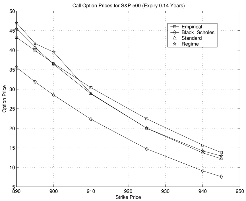
Figure 1: Graph of Table 1 for Options with Expiry of 0.14 Years

The numerical experiments give option pricing results for state one, from four different quote periods over a range of strikes and expiries. We see that regime based option pricing provides lower average percentage error compared to Black-Scholes or standard Fouque option pricing. In fact the average Black-Scholes option pricing error is 30.3% whereas Fouque’s standard and regime based average option pricing errors are 10.6% and 9.9% respectively.

The average Black-Scholes option pricing error of 30.3% over different expiries and strikes validates Fouque’s perturbation solution to stochastic volatility option pricing. Since the option price C is solved by the perturbation expansion equation (54) therefore C should be approximately equal to the leading order term $C_{0}$, which is the Black-Scholes option price. Additionally, it supports our claim that $C_{0}$ can be used as an approximation for intra-regime option prices.

Figure 1 plots table 1 for options with expiry of 0.14 years, with the empirical option prices labelled “empirical”. It is reassuring that all three pricing methods follow the same trend as empirical option prices, providing evidence that all three are viable option pricing methods. We observe that the Black-Scholes option prices consistently underprice over all strikes compared to the empirical prices, which has been frequently observed by many researchers. For instance, the Black-Scholes underpricing is most easily noticeable when empirical option prices exhibit volatility smiles.

The Black-Scholes underpricing has been explained by researchers recognising that Black-Scholes option pricing assumes constant volatility and therefore no risk premium can be associated with any “volatility risk”. In stochastic volatility our risk premium associated with volatility is accounted for by the market price of volatility risk term, therefore it is possible to price options with volatility risk. In Fouque’s perturbation solution to option pricing, $C_{1}$ contains the market price of volatility risk, therefore suffers less from underpricing compared to the Black-Scholes equation.

4.3 State 2 Option Pricing Results

We present the results of our option pricing numerical experiments in state two.

Table 5: Option Pricing Results for S&P 500 Call Option

Expiry	Strike	Empirical	Option Pricing Method
		Price	Black-Scholes	Perturbation Method
(Years)	(Cents)	(Cents)	Pricing	Standard	Regime Based
0.12	1250	75.6	49.7	94.3	92.8
0.12	1275	59.4	32.5	58.4	58.2
0.12	1300	44.6	19.4	35.7	35.6
0.21	1250	89.9	59.5	106.5	105.2
0.21	1275	73.9	42.7	75.1	74.8
0.21	1285	68.0	36.9	65.4	65.3
0.21	1300	59.1	29.2	53.1	53.1
0.45	1250	122.6	84.1	143.7	142.0
0.45	1275	106.9	67.6	115.3	114.7
0.45	1300	91.8	53.2	93.1	93.0
0.72	1250	150.5	107.0	180.2	178.0
0.72	1275	135.0	90.5	152.1	151.0
0.72	1300	120.0	75.6	129.1	128.7
0.97	1300	145.4	95.1	160.0	159.2
		Average Percentage	39.4%	11.2%	10.6%
		Error

Table 6: Option Pricing Results for S&P 500 Call Option

Expiry	Strike	Empirical	Option Pricing Method
		Price	Black-Scholes	Perturbation Method
(Years)	(Cents)	(Cents)	Pricing	Standard	Regime Based
0.14	1200	66.9	50.7	82.5	81.3
0.14	1210	60.1	43.5	68.5	67.8
0.14	1225	50.6	33.8	51.7	51.5
0.14	1250	36.9	20.8	31.3	31.3
0.23	1200	80.2	60.7	93.4	92.3
0.23	1225	64.3	44.3	66.3	66.1
0.23	1250	50.3	30.9	46.7	46.7
0.40	1200	98.5	75.6	112.8	111.7
0.40	1225	83.0	59.6	87.9	87.5
0.40	1250	68.9	45.8	68.5	68.4
0.65	1225	105.4	78.9	112.8	114.5
		Average Percentage	32.1%	9.6%	9.0%
		Error

Table 7: Option Pricing Results for S&P 500 Call Option

Expiry	Strike	Empirical	Option Pricing Method
		Price	Black-Scholes	Perturbation Method
(Years)	(Cents)	(Cents)	Pricing	Standard	Regime Based
0.08	1175	50.9	41.1	62.3	61.2
0.08	1200	32.9	23.6	34.2	34.1
0.08	1225	20.5	11.6	17.5	17.5
0.17	1175	64.4	50.5	71.6	70.8
0.17	1190	55.0	40.2	56.7	56.4
0.17	1200	47.1	34.1	48.5	46.3
0.17	1210	41.3	28.6	41.3	41.3
0.17	1225	33.8	21.5	32.4	32.3
0.17	1240	26.9	15.7	25.3	25.1
0.42	1175	90.3	70.1	96.7	96.0
		Average Percentage	30.0%	7.3%	6.9%
		Error

Table 8: Option Pricing Results for S&P 500 Call Option

Expiry	Strike	Empirical	Option Pricing Method
		Price	Black-Scholes	Perturbation Method
(Years)	(Cents)	(Cents)	Pricing	Standard	Regime Based
0.11	1060	63.4	40.6	80.6	79.2
0.11	1070	56.7	33.2	64.3	63.7
0.11	1075	53.3	29.8	57.7	57.3
0.11	1080	50.2	26.6	51.8	51.6
0.11	1090	44.1	20.9	42.1	42.0
0.11	1100	37.8	15.9	34.4	34.4
0.11	1125	26.3	7.3	21.7	21.2
0.18	1100	48.7	22.3	47.2	47.2
0.18	1125	36.0	12.6	34.6	34.2
0.28	1160	83.4	52.3	97.2	96.4
0.28	1100	59.0	29.0	60.5	60.5
0.28	1125	46.1	18.6	47.5	47.3
		Average Percentage
		Error	51.5%	9.4%	9.1%

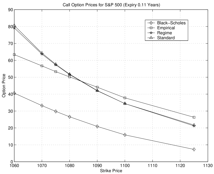
Figure 2: Graph of Table 8 for Options with Expiry of 0.11 Years

The numerical experiments give option pricing results for state two, from four different quote periods over a range of strikes and expiries. As in state one regime based option pricing provides lower average percentage error compared to Black-Scholes or standard Fouque option pricing. In fact the average Black-Scholes option pricing error is 38.2% whereas Fouque’s standard and regime based average option pricing errors are 9.4% and 8.9% respectively. Therefore the pricing error under Black-Scholes option pricing is higher in state two than in state one, which is consistent with empirical observations as volatility smiles increase during “down states” (state two) and therefore option prices deviate away from a constant volatility assumption.

Figure 2 plots table 5 for options with expiry of 0.11 years with the empirical option prices labelled “empirical”. As in state one, all three pricing methods follow the same trend as empirical option prices, providing evidence that all three are viable option pricing methods in state two. We also note the Black-scholes option prices are consistently underpricing over all strikes, as in state one, for the same reasons as in state one -Black-Scholes option pricing does not take into account “volatility risk”.

From figure 2 we observe that both Fouque based option pricing methods exhibit a more pronounced volatility smiling effect compared to figure 1. Since we price options upto the first correction $\sqrt{\epsilon}C_{1}$ and $C_{0}$ does not take into account any volatility smiling effects, we can attribute the smiling effect to $\sqrt{\epsilon}C_{1}$. The term $\sqrt{\epsilon}C_{1}$ can increase volatility smiling through an increase in the market price of volatility risk, which is likely because state two models the “down” state and we expect risk associated with volatility to be higher. Additionally, we notice that $\sqrt{\epsilon}C_{1}$ contains $\rho$, the correlation between the volatility’s Wiener process $W_{2}$ and $W_{1}$, which may increase in “down” states compared to “up” states. This is consistent with empirical observations since volatility tends to increase during a down state.

5 Conclusions

It can be seen from our literature review of volatility models that the development of volatility models has progressed in a logical order to address key shortcomings of previous models. Time dependent models addressed option prices varying with expiration dates, local volatility also addressed volatility smiles and the leverage effect, whereas stochastic volatility could incorporate all the effects captured by local volatility and a range of other empirical effects e.g. greater variability in observed volatility. However the trade-off associated with improved volatility modelling has been loss of analytical tractability.

In conclusion we have shown that Fouque’s option pricing method provides significantly better option pricing accuracy compared to Black-Scholes option pricing over a variety of strikes and expiries. We have provided option prices and have shown that taking into account regime specific $\bar{\sigma}_{i}$, rather than using one $\bar{\sigma}$, improves option pricing accuracy.

References

- AK [08] C. Alexander and A. Kaeck. Regime dependent determinants of credit default swap spreads. Journal of Banking and Finance, 32(6):637–648, 2008.
- Ale [04] C. Alexander. Normal mixture diffusion with uncertain volatility: modelling short and long term smile effects. Journal of Banking and Finance, 28(12):2957–2980, 2004.
- Bac [00] L. Bachelier. Theorie de la speculation (thesis). Annales Scientifiques de l Éole Normale Superieure, 3(17):21–86, 1900.
- BD [07] P. Boyle and T. Draviam. Pricing exotic options under regime switching. Insurance Mathematics and Economics, 40(2):267–282, 2007.
- BM [00] D. Brigo and F. Mercurio. A mixed-up smile. Risk, 13(9):123–126, 2000.
- BO [99] C.M. Bender and S.A. Orszag. Advanced Mathematical Methods for Scientists and Engineers I: Asymptotic Methods and Perturbation Theory. Springer, 1999.
- CR [76] J.C. Cox and S.A. Ross. The Valuation of Options for Alternative Stochastic Processes. Journal of Financial Economics, 3(1), 1976.
- DK [94] E. Derman and I. Kani. Riding on a smile. Risk, 7(2):32–39, 1994.
- DM [94] J.M. Durland and T.H. McCurdy. Duration-Dependent Transitions in a Markov Model of US GNP Growth. Journal of Business and Economic Statistics, 12(3):279–288, 1994.
- Dup [94] B. Dupire. Pricing with a smile. Risk, 7(1):18–20, 1994.
- Dup [97] B. Dupire. Pricing and hedging with smiles. Mathematics of Derivative Securities, 1(1):103–111, 1997.
- Dur [07] G.B. Durham. SV mixture models with application to S&P 500 index returns. Journal of Financial Economics, 85(3):822–856, 2007.
- ECS [05] R.J. Elliott, L. Chan, and T.K. Siu. Option pricing and Esscher transform under regime switching. Annals of Finance, 1(4):423–432, 2005.
- EH [90] C. Engel and J.D. Hamilton. Long Swings in the Dollar: Are They in the Data and Do Markets Know It? American Economic Review, 80(4):689–713, 1990.
- Eng [82] R.F. Engle. Autoregressive Conditional Heteroscedasticity with Estimates of the Variance of United Kingdom Inflation. Econometrica, 50(4):987–1007, 1982.
- EvdH [97] R.J. Elliott and J. van der Hoek. An application of hidden Markov models to asset allocation problems. Finance and Stochastics, 1(3):229–238, 1997.
- [17] J.P. Fouque, G. Papanicolaou, and K.R. Sircar. Derivatives in Financial Markets with Stochastic Volatility. Cambridge University Press New York, 2000.
- [18] J.P. Fouque, G. Papanicolaou, and K.R. Sircar. Mean-reverting stochastic volatility. International Journal of Theoretical and Applied Finance, 3(1):101–142, 2000.
- GL [93] T.J. George and F.A. Longstaff. Bid-Ask Spreads and Trading Activity in the S&P 100 Index Options Market. Journal of Financial and Quantitative Analysis, 28(3):381–397, 1993.
- Ham [89] J.D. Hamilton. A New Approach to the Economic Analysis of Nonstationary Time Series and the Business Cycle. Econometrica, 57(2):357–384, 1989.
- Har [01] M.R. Hardy. A Regime-Switching Model of Long-Term Stock Returns. North American Actuarial Journal, 5(2):41–53, 2001.
- Hes [93] S.L. Heston. A Closed-Form Solution for Options with Stochastic Volatility with Applications to Bond and Currency Options. Review of Financial Studies, 6(2):327–43, 1993.
- Hin [91] E.J. Hinch. Perturbation Methods. Cambridge University Press, 1991.
- Hon [03] T. Honda. Optimal portfolio choice for unobservable and regime-switching mean returns. Journal of Economic Dynamics and Control, 28(1):45–78, 2003.
- HS [94] J.D. Hamilton and R. Susmel. Autoregressive Conditional Heteroskedasticity and Changes in Regime. Journal of Econometrics, 64(1-2):307–33, 1994.
- HW [87] J. Hull and A. White. The Pricing of Options on Assets with Stochastic Volatilities. The Journal of Finance, 42(2):281–300, 1987.
- JS [87] H. Johnson and D. Shanno. Option Pricing when the Variance is Changing. The Journal of Financial and Quantitative Analysis, 22(2):143–151, 1987.
- Kan [79] D. Kannan. An introduction to stochastic processes. New York: North Holland, 1979.
- Kre [93] E. Kreyszig. Advanced Engineering Mathematics. John Wiley & Sons, 1993.
- KS [04] M. Kalimipalli and R. Susmel. Regime-switching stochastic volatility and short-term interest rates. Journal of Empirical Finance, 11(3):309–329, 2004.
- KY [95] M.J. Kim and J.S. Yoo. New index of coincident indicators: A multivariate Markov switching factor model approach. Journal of Monetary Economics, 36(3):607–630, 1995.
- Lei [99] D.P.J. Leisen. Valuation of Barrier Options in a Black-Scholes Setup with Jump Risk. European Finance Review, 3(3):319–342, 1999.
- LH [92] R.G. Lipsey and C.D. Harbury. First Principles of Economics. Oxford University Press, 1992.
- Mar [06] C. Mari. Regime-switching characterization of electricity prices dynamics. Physica A: Statistical Mechanics and its Applications, 371(2):552–564, 2006.
- Mer [73] R.C. Merton. Theory of rational option pricing. Bell Journal of Economics and Management Science, 4(1):141–183, 1973.
- MGPG [06] C. Melodelima, L. Guéguen, D. Piau, and C. Gautier. A computational prediction of isochores based on hidden Markov models. Gene, 385(1):41–49, 2006.
- [37] R.S. Mamon and M.R. Rodrigo. Explicit solutions to European options in a regime-switching economy. Operations Research Letters, 33(6):581–586, 2005.
- [38] M. Musiela and M. Rutkowski. Martingale Methods In Financial Modelling. Springer, 2005.
- Osb [59] M.F.M. Osborne. Brownian Motion in the Stock Market. Operations Research, 7(2):145–173, 1959.
- Pin [03] S. Pinder. An empirical examination of the impact of market microstructure changes on the determinants of option bid-ask spreads. International Review of Financial Analysis, 12(5):563–577, 2003.
- Reb [04] R. Rebonato. Volatility and Correlation: The Perfect Hedger and the Fox. Wiley & Sons, Chichester, UK, 2004.
- RT [96] E. Renault and N. Touzi. Option Hedging and Implied Volatilities in a Stochastic Volatility Model. Mathematical Finance, 6(3):279–302, 1996.
- Sam [65] P.A. Samuelson. Proof that properly anticipated prices fluctuate randomly. Industrial Management Review, 6(2):41–49, 1965.
- Sch [81] R. Schiller. The Uses of Volatility Measures in Assessing Market Efficiency. Journal of Finance, 36(2):291–304, 1981.
- Sch [89] G.W. Schwert. Why Does Stock Volatility Change Over Time? Journal of Finance, 44(5):1115–1153, 1989.
- Sch [90] G.W. Schwert. Stock volatility and the crash of’87. Review of Financial Studies, 3(1):77–102, 1990.
- Sco [87] L.O. Scott. Option Pricing when the Variance Changes Randomly: Theory, Estimation, and an Application. The Journal of Financial and Quantitative Analysis, 22(4):419–438, 1987.
- SF [06] T. Salih and K. Fidanboylu. Modeling and analysis of queuing handoff calls in single and two-tier cellular networks. Computer Communications, 29(17):3580–3590, 2006.
- SM [98] J.G. Simmonds and J.E. Mann. A First Look at Perturbation Theory. Dover Publications, 1998.
- Smi [02] D.R. Smith. Markov-Switching and Stochastic Volatility Diffusion Models of Short-Term Interest Rates. Journal of Business and Economic Statistics, 20(2):183–97, 2002.
- SS [91] E. Stein and J. Stein. Stock price distributions with stochastic volatility: an analytic approach. Review of Financial Studies, 4(4):727–752, 1991.
- SSS [02] M. Sola, F. Spagnolo, and N. Spagnolo. A test for volatility spillovers. Economics Letters, 76(1):77–84, 2002.
- TG [01] E. Trentin and M. Gori. A survey of hybrid ANN/HMM models for automatic speech recognition. Neurocomputing, 37(1-4):91–126, 2001.
- Tim [00] A. Timmermann. Moments of Markov switching models. Journal of Econometrics, 96(1):75–111, 2000.
- TK [84] H.M. Taylor and S. Karlin. An introduction to stochastic modeling. Academic Press San Diego, 1984.
- VPHS [04] P.L. Valls-Pereira, S. Hwang, and S.E. Satchell. How persistent is volatility? An answer with stochastic volatility models with Markov regime switching state equations. Journal of Business Finance and Accounting, 34(5-6):1002–1024, 2004.
- W+ [98] P. Wilmott et al. Derivatives: the theory and practice of financial engineering. John Wiley & Sons, 1998.