Implementing Loss Distribution Approach for Operational Risk

Abstract

To quantify the operational risk capital charge under the current regulatory framework for banking supervision, referred to as Basel II, many banks adopt the Loss Distribution Approach. There are many modeling issues that should be resolved to use the approach in practice. In this paper we review the quantitative methods suggested in literature for implementation of the approach. In particular, the use of the Bayesian inference method that allows to take expert judgement and parameter uncertainty into account, modeling dependence and inclusion of insurance are discussed.

Keywords: operational risk; loss distribution approach; Bayesian inference; dependence modeling; Basel II.

1 Operational risk under Basel II

Under the current regulatory framework for the banking industry [1], referred to as Basel II, the banks are required to hold adequate capital against operational risk (OR) losses. OR is a new category of risk, in addition to market and credit risks, attracting capital charge and defined by Basel II [1, p.144] as: “[…] the risk of loss resulting from inadequate or failed internal processes, people and systems or from external events. This definition includes legal risk, but excludes strategic and reputational risk.” Similar regulatory requirements for the insurance industry are referred to as Solvency 2. OR is significant in many financial institutions. Examples of extremely large OR losses are: Barings Bank (loss GBP 1.3 billion in 1995), Sumitomo Corporation (loss USD 2.6 billion in 1996), Enron (USD 2.2 billion in 2001), and recent loss in Société Générale (Euro 4.9 billion in 2008). In Basel II, three approaches can be used to quantify the OR annual capital charge $C$, see [1, pp.144-148]:

• The Basic Indicator Approach: $C=\alpha\frac{1}{n}\sum\nolimits_{j=1}^{n}{GI(j)}$, $\alpha=0.15$, where $GI(j)$, $j=1,..,n$ are the annual positive gross incomes over the previous three years.

• The Standardised Approach: $C=\frac{1}{3}\sum\nolimits_{j=1}^{3}{\max[\sum\nolimits_{i=1}^{8}{\beta_{i}GI_{i}(j)},0]}$, where $\beta_{i}$, $i=1,\ldots,8$ are the factors for eight business lines (BL) listed in Table 1 and $GI_{i}(j)$, $j=1,2,3$ are the annual gross incomes of the $i$-th BL in the previous three years.

• The Advanced Measurement Approaches (AMA): a bank can calculate the capital charge using internally developed model subject to regulatory approval.

A bank intending to use the AMA should demonstrate accuracy of the internal models within the Basel II risk cells (eight business lines times seven risk types, see Table 1) relevant to the bank and satisfy some criteria, see [1, pp.148-156], including:

• The use of the internal data, relevant external data, scenario analysis and factors reflecting the business environment and internal control systems;

• The risk measure used for capital charge should correspond to the 99.9% confidence level for a one-year holding period;

• Diversification benefits are allowed if dependence modeling is approved by a regulator;

• Capital reduction due to insurance is capped by 20%.

A popular method under the AMA is the loss distribution approach (LDA). Under the LDA, banks quantify distributions for frequency and severity of OR losses for each risk cell (business line/event type) over a one-year time horizon. The banks can use their own risk cell structure but must be able to map the losses to the Basel II risk cells. There are various quantitative aspects of the LDA modeling discussed in several books [2, 3, 4, 5, 6, 7] and various papers, e.g. [8, 9, 10] to mention a few. The commonly used LDA model for calculating the total annual loss $Z_{(\bullet)}(t)$ in a bank (occurring in the years $t=1,2,\ldots)$ can be formulated as

$$Z_{(\bullet)}(t)=\sum\limits_{j=1}^{J}{Z_{j}(t)};\quad Z_{j}(t)=\sum\limits_{i=1}^{N_{j}(t)}{X_{j}^{(i)}(t)}.$$ (1)

Here, the annual loss $Z_{j}(t)$ in risk cell $j$ is modeled as a compound process over one year with the frequency (annual number of events) $N_{j}(t)$ implied by a counting process (e.g. Poisson process) and random severities $X_{j}^{(i)}(t)$, $i=1,\ldots,N_{j}(t)$. Typically, the frequencies and severities are assumed independent. Estimation of the annual loss distribution by modeling frequency and severity of losses is a well-known actuarial technique, see e.g. Klugman et al.[11]. It is also used to model solvency requirements for the insurance industry, see e.g. Sandström [12] and Wüthrich and Merz [13]. Under the model (1), the capital is defined as the 0.999 Value at Risk (VaR) which is the quantile of the distribution for the next year annual loss $Z_{(\bullet)}(T+1)$:

$$VaR_{q}(Z_{(\bullet)}(T+1))=F_{Z_{(\bullet)}(T+1)}^{-1}(q)=\inf\{z:\Pr[Z_{(\bullet)}(T+1)>z]\leq 1-q\}$$ (2)

at the level $q=0.999$. Here, index $T$+1 refers to the next year and notation $F_{Y}^{-1}(q)$ denotes the inverse distribution of a random variable (rv) $Y$. The capital can be calculated as the difference between the 0.999 VaR and expected loss if the bank can demonstrate that the expected loss is adequately captured through other provisions. If correlation assumptions can not be validated between some groups of risks (e.g. between business lines) then the capital should be calculated as the sum of the 0.999 VaRs over these groups. This is equivalent to the assumption of perfect positive dependence between annual losses of these groups.

In this paper, we review some methods proposed in the literature for the LDA model (1). In particular, we consider the Bayesian inference approach that allows to account for expert judgment and parameter uncertainty which are important issues in operational risk management.

The paper is organised as follows. Section 2 describes the requirements for the data that should be collected and used for Basel II AMA. Section 3 and Section 4 are focused on modeling truncated data and the tail of severity distribution respectively. Calculation of compound distributions is considered in Section 5. In Section 6, we review the estimation of the frequency and severity distributions using frequentist and Bayesian inference approaches. Combining different data sources (internal data, expert judgement and external data) is considered in Section 7. Modeling dependence and insurance are discussed in Section 8 and Section 9 respectively. Finally, Section 10 presents the estimation of the capital charge via full predictive distribution accounting for parameter uncertainty.

2 Data

Basel II specifies requirement for the data that should be collected and used for AMA. In brief, a bank should have: internal data, external data and expert opinion data. In addition, internal control indicators and factors affecting the businesses should be used. Development and maintenance of OR databases is a difficult and challenging task. Some of the main features of the required data are summarized as follows.

Internal data. The internal data should be collected over a minimum five year period to be used for capital charge calculations (when the bank starts the AMA, a three-year period is acceptable). Due to a short observation period, typically, the internal data for many risk cells contain few (or none) high impact low frequency losses. A bank must be able to map its historical internal loss data into the relevant Basel II risk cells in Table 1. The data must capture all material activities and exposures from all appropriate sub-systems and geographic locations. A bank can have an appropriate reporting threshold for internal data collection, typically of the order of Euro 10,000. Aside from information on gross loss amounts, a bank should collect information about the date of the event, any recoveries of gross loss amounts, as well as some descriptive information about the drivers of the loss event.

External data. A bank’s OR measurement system must use relevant external data. These data should include data on actual loss amounts, information on the scale of business operations where the event occurred, and information on the causes and circumstances of the loss events. Industry data are available through external databases from vendors (e.g. Algo OpData provides publicly reported OR losses above USD 1 million) and consortia of banks (e.g. ORX provides OR losses above Euro 20,000 reported by ORX members). The external data are difficult to use directly due to different volumes and other factors. Moreover, the data have a survival bias as typically the data of all collapsed companies are not available. Several Loss Data Collection Exercises (LDCE) for historical OR losses over many institutions were conducted and their analyses reported in the literature. In this respect, two papers are of high importance: Moscadelli [14] analysing 2002 LDCE and Dutta and Perry [15] analysing 2004 LDCE where the data were mainly above Euro 10,000 and USD 10,000 respectively.

Scenario Analysis/expert opinion. A bank must use scenario analysis in conjunction with external data to evaluate its exposure to high-severity events. Scenario analysis is a process undertaken by experienced business managers and risk management experts to identify risks, analyse past internal/external events, consider current and planned controls in the banks; etc. It may involve: workshops to identify weaknesses, strengths and other factors; opinions on the impact and likelihood of losses; opinions on sample characteristics or distribution parameters of the potential losses. As a result some rough quantitative assessment of risk frequency and severity distributions can be obtained. Scenario analysis is very subjective and should be combined with the actual loss data. In addition, it should be used for stress testing, e.g. to assess the impact of potential losses arising from multiple simultaneous loss events.

Business environment and internal control factors. A bank’s methodology must capture key business environment and internal control factors affecting OR. These factors should help to make forward-looking estimation, account for the quality of the controls and operating environments, and align capital assessments with risk management objectives.

3 A note on modeling truncated data

As mentioned above, typically internal data are collected above some low level of the order of Euro 10,000. Generally speaking, omitting data increases uncertainty in modeling but having a reporting threshold helps to avoid difficulties with collection of too many small losses. Often, the data below a reported level are simply ignored in the analysis, arguing that the capital is mainly determined by the low frequency heavy tailed severity risks. However, the impact of data truncation for other risks can be significant. Even if the impact is small often it should be estimated to justify the reporting level. Recent studies of this problem include Frachot et al. [9], Bee [16], Chernobai et al. [17], Mignola and Ugoccioni [18], Luo et al. [19], and Baud et al. [20]. A consistent procedure to adjust for missing data is to fit the data above the threshold using the correct conditional density. To demonstrate, consider one risk cell only, where the loss events follow a Poisson process, so that the annual counts $N(t)$, $t=1,\ldots,T$ are independent and Poisson distributed, $Poisson(\lambda)$, with the probability function

$$p(k|\lambda)=\Pr[N(t)=k]=\frac{\lambda^{k}}{k!}\exp(-\lambda),\quad\lambda>0,\;k=0,1,\ldots\quad.$$ (3)

Assume that the severities $X^{(i)}(t)$ are all independent and identically distributed (iid) from the density $f(x|{{\bm{\beta}}})$ whose distribution is denoted $F(x|{{\bm{\beta}}})$, where ${{\bm{\beta}}}$ is a vector of distribution parameters. Also, assume that the counts and severities are independent. Then the loss events above the level $L$ have iid counts $\tilde{N}(t)$ from $Poisson(\lambda_{L})$, $\lambda_{L}=\lambda(1-F(L|{{\bm{\beta}}}))$ and iid severities $\tilde{X}^{(i)}(t)$ from the conditional density

$$f_{L}(x|{{\bm{\beta}}})=\frac{f(x|{{\bm{\beta}}})}{1-F(L|{{\bm{\beta}}})};\quad L\leq x<\infty.$$ (4)

The joint density (likelihood) of the data ${\rm{\bf Y}}$ over a period of $T$ years (all counts $\tilde{N}(t)$ and severities $\tilde{X}^{(i)}(t)$, $i=1,\ldots,\tilde{N}(t)$, $t=1,\ldots,T)$, at $\tilde{N}(t)=\tilde{n}(t)$ and $\tilde{X}^{(i)}(t)=\tilde{x}^{(i)}(t)$, is

$$l({\rm{\bf y}}|{{\bm{\beta}}},\lambda)=\prod\limits_{t=1}^{T}{p\left({\tilde{n}(t)|\lambda(1-F(L|{{\bm{\beta}}}))}\right)\prod\limits_{i=1}^{\tilde{n}(t)}{f_{L}\left({\tilde{x}^{(i)}(t)|{{\bm{\beta}}}}\right)}}.$$ (5)

Note that here, the conditional density $f_{L}(x|{{\bm{\beta}}})$, rather than $f(x|{{\bm{\beta}}})$, is used. The parameters $({{\bm{\beta}}},\lambda)$ can be estimated, for example, by maximizing the likelihood (5) and their uncertainties can be estimated using the second derivatives of the log-likelihood; see Section 6.1. Then estimated frequency $Poisson(\lambda)$ and severity $f(x|{{\bm{\beta}}})$ densities are used for the annual loss calculations.

In the case of constant threshold, the maximum likelihood estimators (MLEs) for parameters ${{\hat{\bm{\beta}}}}$ and $\hat{\lambda}$ can be calculated marginally, i.e. ${{\hat{\bm{\beta}}}}$ is calculated by maximizing the likelihood of the severities; $\hat{\lambda}_{L}$ is calculated using the average of the observed counts; and finally $\hat{\lambda}=\hat{\lambda}_{L}/(1-F(L|{{\hat{\bm{\beta}}}}))$. However, calculation of their uncertainties will require the use of the full joint likelihood (5). If the observed losses are scaled before fitting or the reporting threshold has changed over time then one should consider a model with the threshold varying in time studied in [21]. In this case the joint estimation of the frequency and severity parameters using full likelihood of the data is required even for parameter point estimators.

Of course, the assumption in the above approach is that missing losses and reported losses are realizations from the same distribution. Thus the method should be used with extreme caution if a large proportion of data is missing.

Ignoring missing data. Ignoring missing data will have an impact on risk estimates. For example, using data reported above the threshold, one can fit $Poisson(\lambda_{L})$ frequency and fit the severity using:

• “naive model” – $f(x|{{\bm{\beta}}})$;

• “shifted model” – $f(x-L|{{\bm{\beta}}})$;

• “truncated model” – $f_{L}(x|{{\bm{\beta}}})$.

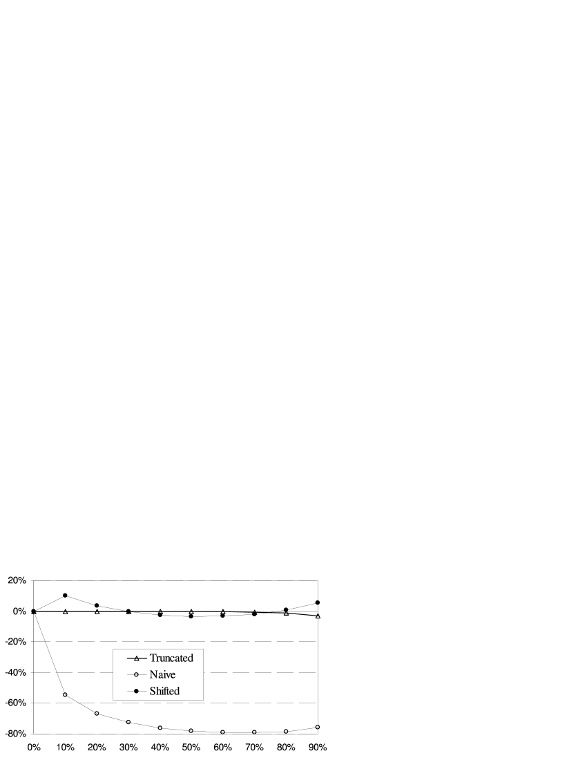
Figure 2: Relative bias in the 0.999 quantile of the annual loss vs % of truncated points for several models ignoring truncation in the case of heavier tail severities from $LN(3,2)$. The annual counts above the truncation level are from $Poisson(10)$.

Calculation of the annual loss quantile using incorrect frequency and severity distributions will induce a bias. Figure 1 and Figure 2 show the relative bias in the 0.999 annual loss quantile (relative difference between the 0.999 quantiles under the false and true models) vs a fraction of truncated points for the cases of light and heavy tail severities respectively. In this example, the severity is from Lognormal distribution, $LN(\mu,\sigma)$, i.e. log-severity $\ln X^{(i)}(t)$ is from the Normal distribution, $Normal(\mu,\sigma)$, with mean $\mu$ and standard deviation $\sigma$. The parameter values are chosen the same as some cases considered in [19]. In particular: Figure 1 is the case of $\lambda_{L}=10$ and $\sigma=1$; and Figure 2 is the case of $\lambda_{L}=10$ and $\sigma=2$. The latter corresponds to the heavier tail severity. Here, the calculated bias is due to the model error only, i.e. corresponds to the case of a very large data sample. Also note, that the actual value of the scale parameter $\mu$ is not relevant because only relative quantities are calculated. “Naive model” and “shifted model” are easy to fit but induced bias can be very large. Typically: “naive model” leads to a significant underestimation of the capital, even for a heavy tail severity; “shifted model” is better than “naive model” but worse then “truncated model”; the bias from “truncated model” is less for heavier tail severities.

4 Modeling severity tail

Due to simple fitting procedure, one of the popular distributions to model severity is Lognormal. It is a heavy tail distribution, i.e. belongs to the class of so-called sub-exponential distributions where the tail decays slower than any exponential tail. Often, it provides a reasonable overall statistical fit as reported in the literature, see e.g. [15]. Also, it was suggested for OR at the beginning of Basel II development, see [22, p.34]. However, due to the high quantile level requirement for OR capital charge, accurate modeling of extremely high losses (the tail of severity distribution) is critical and other heavy tail distributions are often considered to be more appropriate. Two studies of OR data collected over many institutions are of central importance here: Moscadelli [14] analysing 2002 LDCE (where Extreme Value Theory (EVT) is used for analysis in addition to some standard two parameter distributions) and Dutta and Perry [15] analysing 2004 LDCE. The latter paper considered the four-parameter g-and-h and GB2 distributions as well as EVT and several two parameter distributions.

EVT–threshold exceedances. There are two types of EVT models: traditional block maxima (modeling the largest observation) and threshold exceedances. The latter is often used to model the tail of OR severity distribution and is briefly described below; for more details see McNeil et al. [6] and Embrechts et al. [23]. Consider a rv $X$, whose distribution is $\Pr[X\leq x]=F(x)$. Given a threshold $u$, the exceedance of $X$ over $u$ is distributed from

$$F_{u}(y)=\Pr[X-u\leq y|X>u]=\frac{F(y+u)-F(u)}{1-F(u)}.$$ (6)

Under quite general conditions, as the threshold $u$ increases, the excess distribution $F_{u}(.)$ converges to a generalized Pareto distribution (GPD)

$$G_{\xi,\beta}(y)=\left\{{{\begin{array}[]{*{20}c}{1-(1+\xi y/\beta)^{-1/\xi};\;\;\xi\neq 0,\hfill}\\ {1-\exp(-y/\beta);\;\quad\xi=0.\hfill}\\ \end{array}}}\right.$$ (7)

That is we can find a function $\beta(u)$ such that

$$\mathop{\lim}\limits_{u\to a}\;\mathop{\sup}\limits_{0\leq y\leq a-u}|F_{u}(y)-G_{\xi,\beta(u)}(y)|=0,$$

where $a\leq\infty$ is the right endpoint of $F(x)$, $\xi$ is the shape parameter and $\beta>0$ is the scale parameter. Also, $y\geq 0$ when $\xi\geq 0$ and $0\leq y\leq-\beta/\xi$ when $\xi<0$. The GPD case $\xi=0$ corresponds to an exponential distribution. If $\xi>0$, the GPD is heavy tailed and some moments do not exist. In particular, if $\xi\geq 1/m$ then the $m$-th and higher moments do not exist. The analysis of OR data in [14] reported even the cases of $\xi\geq 1$ for some business lines, i.e. infinite mean distributions; also see discussions in Nešlehová et al. [24]. It seems that the case of $\xi<0$ is not relevant to modeling OR as all reported results indicate non-negative shape parameter. Though, one could think of a risk control mechanism restricting the losses by an upper level and then the case of $\xi<0$ might be relevant.

In the context of OR, given iid losses $X^{(k)}$, $k=1,2,\ldots,K$ one can chose a threshold $u$ and model the losses above the threshold using GPD (7) and the losses below using empirical distribution, i.e.

$$F(x)\approx\left\{{{\begin{array}[]{c}{G_{\xi,\beta}(x-u)(1-F_{n}(u))+F_{n}(u);\;\;x\geq u,}\\ {F_{n}(x)=\frac{1}{K}\sum\nolimits_{k=1}^{K}{I(X^{(k)}\leq x)};\quad x<u.}\end{array}}}\right.$$ (8)

Here, $I(.)$ is an indicator function. There are various ways to fit the GPD parameters including the Bayesian inference and maximum likelihood methods; see Section 6 and Embrechts et al. [23, Section 6.5]. The approach (8) is a so-called splicing method when the density is modeled as

$$f(x)=w_{1}f_{1}(x)+w_{2}f_{2}(x),\quad w_{1}+w_{2}=1,$$ (9)

where $f_{1}(x)$ and $f_{2}(x)$ are proper density functions defined on $x<L$ and $x\geq L$ respectively. In (8), $f_{1}(x)$ is modeled by the empirical distribution but one may choose a parametric distribution instead. Splicing can be viewed as a mixture of distributions defined on non-overlapping regions while a standard mixture distribution is a combining of distributions defined on the same range. The choice of the threshold $u$ is critical, for details of the methods to choose a threshold we refer to [23, Section 6.5].

g-and-h, GB2 and GCD distributions. A rv $X$ is said to have g-and-h distribution if

$$X=a+b\frac{\exp(gY)-1}{g}\exp(hY^{2}/2),$$ (10)

where $Y$ is a rv from the standard Normal distribution and $(a,b,g,h)$ are the parameters. A comparison of the g-and-h with EVT was studied in Degen et al. [25]. It was demonstrated that for the g-and-h distribution, convergence of the excess distribution to the GPD is extremely slow. Therefore, quantile estimation using EVT may lead to inaccurate results if data are well modeled by the g-and-h distribution.

GB2 (the generalized Beta distribution of the second kind) is another four-parameter distribution that nests many important one- and two-parameter distributions. Its density is defined as

$$f(x)=\frac{|a|x^{ap-1}}{b^{ap}B(p,q)[1+(x/b)^{a}]^{p+q}},\quad x>0,$$ (11)

where $B(p,q)$ is the Beta function and ($a$,$b$,$p$,$q)$ are parameters. Both g-and-h and GB2 four parameter distributions were used in [15] as the alternative to EVT.

A convenient distribution recently suggested for OR in [26] is Generalized Champernowne distribution (GCD) with the density defined as

$$f(x)=\frac{\alpha(x+c)^{\alpha-1}((M+c)^{\alpha}-c^{\alpha})}{((x+c)^{\alpha}+(M+c)^{\alpha}-2c^{\alpha})^{2}},\;x\geq 0$$ (12)

and parameters $\alpha>0$, $M>0$, $c\geq 0$. It behaves as Lognormal in a middle and as Pareto in the tail.

5 Calculating compound distribution

If the severity and frequency distributions and their parameters are known then, in general, the distribution $H(.)$ of the annual loss

$$Z=\sum_{i=1}^{N}{X^{(i)}}$$ (13)

should be calculated numerically. Here, we assume that severities $X^{(i)}$ are iid from the distribution $F(x)$ and the frequency $N$, with $p_{n}=\mathrm{Pr}[N=n]$, is independent from the severities. Most popular numerical methods are Monte Carlo, Panjer recursion and FFT methods described below. Also, there are several approximations discussed below too.

5.1 Monte Carlo method.

The easiest to implement is Monte Carlo method with the following logical steps:

1. For $k=1,\ldots,K$

   1. Simulate the annual number of events $N$ from the frequency distribution.

   2. Simulate independent severities $X^{(1)},\ldots,X^{(N)}$ from the severity distribution.

   3. Calculate $Z^{(k)}=\sum\nolimits_{i=1}^{N}{X^{(i)}}$.

2. Next $k$

Obtained $Z^{(1)},\ldots,Z^{(K)}$ are samples from a compound distribution $H(.)$. The 0.999 quantile and other distribution characteristics can be estimated using the simulated samples in the usual way. Denote the samples $Z^{(1)},\ldots,Z^{(K)}$ sorted into ascending order as $\tilde{Z}^{(1)}\leq\ldots\leq\tilde{Z}^{(K)}$, then the quantile $H^{-1}(q)$ can be estimated by $\tilde{Z}^{(\left\lfloor{Kq+1}\right\rfloor)}$. Here, $\left\lfloor.\right\rfloor$ denotes rounding downward. The numerical error (due to the finite number of simulations $K$) in the quantile estimator can be assessed by forming a conservative confidence interval $[\tilde{Z}^{(r)},\tilde{Z}^{(s)}]$ to contain the true value with probability $\gamma$. This can be done by utilizing the fact that the number of samples not exceeding the quantile $H^{-1}(q)$ has a Binomial distribution with parameters $q$ and $K$ (i.e. with $\mathrm{mean}=Kq$ and ${\mathrm{var}}=Kq(1-q))$. Approximating the Binomial by the Normal distribution leads to a simple formula:

$$\begin{array}[]{l}r=\left\lfloor l\right\rfloor{\kern 1.0pt}{\kern 1.0pt},\;\;l=Kq-F_{N}^{-1}((1+\gamma)/2)\sqrt{Kq(1-q)},\\ s=\left\lceil u\right\rceil{\kern 1.0pt},\;\;u=Kq+F_{N}^{-1}((1+\gamma)/2)\sqrt{Kq(1-q)},\\ \end{array}$$ (14)

where $\left\lceil.\right\rceil$ denotes rounding upwards and $F_{N}^{-1}$ is the standard Normal distribution. The above formula works very well for $Kq(1-q)\gtrsim 50$.

A large number of simulations, typically $K\geq 10^{5}$, should be used to get a good numerical accuracy for the 0.999 quantile. However, a priori, the number of simulations required to achieve a specific accuracy is not known. One of the approaches is to continue simulations until a numerical error, calculated using (14), achieves the desired level.

5.2 FFT and Panjer recursion.

Although Monte Carlo is straightforward and robust, it is slow to get accurate results. High precision results are especially important for sensitivity studies, where the first or even the second order derivatives are involved. Fast Fourier Transform (FFT) and Panjer recursion are the other two popular alternatives to calculate the distribution of compound loss (13). Both have a long history, but their applications to computing very high quantiles of the compound distributions in the case of high frequencies or heavy tail severities are relatively recent developments in the area of quantitative risk.

Panjer recursion. The Panjer recursion is based on calculating the compound distribution via convolutions. Using a well known fact that the distribution of the sum of two independent continuous random variables can be calculated as convolution, the compound distribution of the annual loss $Z$ can be calculated as

$$H(z)=\sum_{k=0}^{\infty}\Pr[Z\leq z|N=k]\Pr[N=k]=\sum_{k=0}^{\infty}p_{k}F^{(k)}(z),$$ (15)

where $F^{(k)}(z)=\Pr[X_{1}+\cdots+X_{k}\leq z]$ is the $k$th convolution of $F$ calculated recursively as

$$F^{(k)}(z)=\int_{0}^{z}F^{(k-1)}(z-x)f(x)dx$$

with $F^{(0)}(z)=1$, $z\geq 0$ and $F^{(0)}(z)=0$, $z<0$. Note that integration limits are $0$ and $z$ because severities considered are nonnegative. Thought the formula is analytic, its direct calculation is difficult as the convolution powers are not available in closed form in general. Panjer recursion is a very efficient method to calculate (15) in the case of Poisson, negative binomial and binomial frequency distributions and discrete severities. More precisely, the frequency distribution should belong to a Panjer class $(a,b,1)$, i.e. to satisfy

$$p_{n}=\left(a+b/n\right)p_{n-1},\quad\mbox{for }n\geq 2.$$ (16)

The continuous severity distribution $F(x)$ can be discretized on $\{0,\Delta,2\Delta,\ldots\}$, by choosing a unit $\Delta>0$ and defining discrete density $f_{n}=\mathrm{Pr}[X=n\Delta]$ as e.g.

$$f_{0}=F(\Delta/2),\quad f_{n}=F(n\Delta+\Delta/2)-F(n\Delta-\Delta/2),\quad n=1,2,\ldots.$$ (17)

Then the discrete compound density $h_{n}=\mathrm{Pr}[Z=n\Delta]$ can be calculated recursively as

$$h_{n}=\frac{(p_{1}-(a+b)p_{0})f_{n}+\sum_{j=1}^{n}\left(a+bj/n\right)f_{j}h_{n-j}}{1-af_{0}},\quad n\geq 1$$ (18)

with $h_{0}=\sum\limits_{k=0}^{\infty}{(f_{0})^{k}p_{k}}$. The corresponding discrete distribution converges to the true continuous distribution $H(z)$ weakly as $\Delta\rightarrow 0$ and the number of required operations is of the order of $O(n^{2})$ (in comparison with $O(n^{3})$ of explicit convolution). Detailed description of this method can be found in [5, Section 6.6] and generalized versions of Panjer recursion are discussed in [27], [28], [29].

FFT method. The characteristic function (CF) of the compound loss $Z$ can be calculated as

$$\chi(t)=\sum\limits_{k=0}^{\infty}{[\varphi(t)]^{k}p_{k}}=\psi(\varphi(t)),$$ (19)

where $\varphi(t)$ is the CF of the severity density $f(x)$: $\varphi(t)=\int\nolimits_{-\infty}^{\infty}{f(x)\exp(itx)dx}$ and $\psi(s)$ is the probability generating function of the frequency distribution: $\psi(s)=\sum\nolimits_{k=0}^{\infty}{s^{k}p_{k}}$. For example, in the case of $N$ distributed from $Poisson(\lambda)$, $\chi(t)=\exp(\lambda\varphi(t)-\lambda)$. Given CF, the density of $Z$ can be calculated via the inverse Fourier transform as $h(z)=\frac{1}{2\pi}\int\nolimits_{-\infty}^{\infty}{\chi(t)\exp(-itz)dt}$. For severity discretized as $(f_{0},f_{1},\ldots,f_{M-1})$, e.g. using (17), the continuous Fourier transform is reduced to the discrete Fourier transformation (DFT)

$$\varphi_{k}=\sum_{m=0}^{M-1}f_{m}\exp\left(\frac{2\pi m}{M}k\right),\quad k=0,1,\ldots,M-1.$$ (20)

Then the compound loss discrete CF $\chi_{k}=\psi(\varphi_{k})$, $k=0,\ldots,M-1$ is calculated and the discrete density $h_{k}$ is recovered from $\chi_{k}$ by the inverse transformation

$$h_{n}=\frac{1}{M}\sum_{k=0}^{M-1}\chi_{k}\exp\left(-\frac{2\pi k}{M}n\right),\quad n=0,1,\ldots,M-1.$$ (21)

FFT is a method that allows to calculate the above DFTs (20-21) efficiently using $O(M\log_{2}M)$ operations, when $M=2^{r}$ with a positive integer $r$; see e.g. [30, Chapter 12] for details and code. A commonly recognised pitfall of FFT in evaluating compound distribution, which was recently studied in great detail in [31, 32], is the so-called aliasing error. To explain, assume that there is no truncation error in severity discretisation, then FFT procedure calculates the compound distribution on $m=0,\ldots,M-1$, i.e. the mass of compound distribution beyond $M-1$ is “wrapped” into the range $m=0,\ldots,M-1$. This error is larger for heavy tailed severities. Choosing $M$ much larger than the required quantile to reduce this error is very inefficient and the recommended procedure is to use tilting, the transformation increasing the severity tail decay that commutes with convolution. The tilting transforms the severity as $\tilde{f}_{j}=\exp(-j\theta)f_{j},\quad j=0,\ldots,M-1$. Then FFT calculation of the compound distribution (20-21) is performed using transformed severity and the final result $\tilde{h}_{j}$ is adjusted to get the compound distribution $h_{j}=\tilde{h}_{j}\exp(\theta j)$. It was reported that the choice $\theta\approx 20/M$ for standard double precision (8 bytes) calculations works well.

The Panjer recursion has often been compared with FFT, and it is accepted that the former is slower if the grid size is large, see e.g. [31]. Both methods have discretization error. Note that, Panjer recursion has no truncation error presented in FFT. Also note that, FFT can be used in general for any frequency and severity distributions while Panjer recursion is restricted to non-negative severities and a special class of frequency distributions. Typically, both methods are faster than Monte Carlo by a factor of few orders. Other methods to calculate the compound distribution include direct integration of the CF [33] and a hybrid method combining Panjer recursion, importance sampling and trans-dimensional Markov chain Monte Carlo considered in [34].

5.3 Closed-form approximation

The moments of compound distributions can be expressed via the moments of frequency and severity distributions. This can be utilized to approximate the compound loss using e.g. Normal or translated Gamma distributions by matching two or three moments respectively, see e.g. [6, Section 10.2.3]. Of course for heavy tailed distributions and high quantiles these approximations do not work well (note that low order moments may not even exist for some ORs). If the severities $X^{(i)}$ are iid from the sub-exponential (heavy tail) distribution $F(.)$, then the tail of the compound distribution $H(.)$ is related to the severity tail as

$$1-H(z)\sim E[N](1-F(z)),\quad z\to\infty,$$ (22)

see e.g. [23, Theorem 1.3.9]. Here, “$\sim$” means that the ratio of the left- and right-hand sides converge to 1. The validity of this asymptotic result was demonstrated for the cases when $N$ is distributed from Poisson, binomial or negative binomial. This approximation can be used to calculate the quantiles of the annual loss as

$$VaR_{q}(Z)\sim F^{-1}\left({1-\frac{1-q}{E[N]}}\right),\quad q\to 1.$$ (23)

For application in the OR context, see Böcker and Klüppelberg [35]. Under the assumption that the severity has finite mean, Böcker and Sprittulla [36] derived a correction reducing the approximation error of (23).

6 Model fitting

Estimation of the frequency and severity distributions is a challenging task, especially for low frequency high impact losses, due to very limited data for some risks. The main tasks involved into the fitting are: finding the best point estimates for the distribution parameters, quantification of the parameter uncertainties, assessing the model quality (model error). In general, these tasks can be accomplished by undertaking either the so-called frequentist or Bayesian approaches briefly discussed below.

6.1 Frequentist approach

Fitting distribution parameters using data via the frequentist approach is a classical problem described in many textbooks. For the purposes of this review it is worth to mention several aspects and methods. Firstly, under the frequentist approach one says that the model parameters are fixed while their estimators have associated uncertainties that typically converge to zero when a sample size increases. Several popular methods to fit parameters of the assumed distribution are:

• method of moments – matching the observed moments;

• matching certain quantiles of empirical distribution;

• maximum likelihood – find parameter values that maximize the joint likelihood of data;

• estimating parameters by minimizing a certain distance between empirical and theoretical distributions, e.g. Anderson-Darling or other statistics, see Ergashev [37].

The most popular approach is the maximum likelihood method. Here, given the model parameters ${{\bm{\theta}}}=(\theta_{1},\theta_{2},\ldots)$, assume that the joint density (likelihood) of data ${\rm{\bf Y}}=(Y_{1},\ldots,Y_{n})$ is known in functional form $\ell({\rm{\bf y}}|{{\bm{\theta}}})$. Then the maximum likelihood estimators (MLEs) ${{\hat{\bm{\theta}}}}^{MLE}$ are the values of the parameters ${{\bm{\theta}}}$ maximizing $\ell({\rm{\bf y}}|{{\bm{\theta}}})$. Often it is assumed that $Y_{1},\ldots,Y_{n}$ are iid from $f(.|{{\bm{\theta}}})$; then the likelihood is $\ell({\rm{\bf y}}|{{\bm{\theta}}})=\prod\limits_{i=1}^{n}{f(y_{i}|{{\bm{\theta}}})}$. The uncertainty of the MLEs can be estimated using the asymptotic result that: under suitable regularity conditions, as the sample size increases, ${{\hat{\bm{\theta}}}}^{MLE}$ converges to ${{\bm{\theta}}}$ and is Normally distributed with the mean ${{\bm{\theta}}}$ and covariance matrix $n^{-1}{\rm{\bf I}}({{\bm{\theta}}})^{-1}$, where

$${\rm{\bf I}}({{\bm{\theta}}})_{km}=-\frac{1}{n}E[\partial^{2}\ln\ell({\rm{\bf Y}}|{{\bm{\theta}}})/\partial\theta_{k}\partial\theta_{m}]$$ (24)

is the expected Fisher information matrix. For precise details on regularity conditions and proofs see e.g Lehmann [38, Theorem 6.2.1 and 6.2.3]. The required regularity conditions are mild but often difficult to prove. Also, whether a sample size is large enough to use this asymptotic result is another difficult question to answer in practice. Often, (24) is approximated by the observed information matrix

$$-\frac{1}{n}\partial^{2}\ln\ell({\mathrm{\bf y}}|{{\bm{\theta}}})/\partial\theta_{k}\partial\theta_{m}=-\frac{1}{n}\sum\nolimits_{i=1}^{n}{\partial^{2}\ln f(y_{i}|{{\bm{\theta}}})/\partial\theta_{k}\partial\theta_{m}}$$ (25)

for a given realization of data ${\mathrm{\bf y}}$. This should converge to the matrix (24) by the law of large numbers. Note that the mean and covariances depend on the unknown parameters ${{\bm{\theta}}}$ and are usually estimated by replacing ${{\bm{\theta}}}$ with ${{\hat{\bm{\theta}}}}^{MLE}$ for a given realization of data. This asymptotic approximation may not be accurate enough for small samples.

Another common way to estimate the parameter uncertainties is Bootstrap method. It is based on generating many data samples of the same size from the empirical distribution of the original sample and calculating the parameter estimates for each sample to get the distribution of the estimates. For a good introduction to the method we refer the reader to Efron and Tibshirani [39].

Usually maximization of the likelihood (or minimization of some distances in other methods) should be done numerically. Popular numerical optimization algorithms include: simplex method, Newton methods, expectation maximization (EM) algorithm, simulated annealing. It is worth to mention that the last is attempting to find a global maximum while other methods are designed to find a local maximum only. For the latter, using different starting points helps to find a global maximum. Typically, EM is more stable and robust than the standard deterministic methods such as simplex or Newton methods. To assess the quality of the fit, there are several popular goodness of fit tests including Kolmogorov-Smirnov, Anderson-Darling and chi-square tests. Also, the likelihood ratio test and Akaike’s information criterion are often used to compare models. Again, detailed descriptions of the above mentioned methodologies can be found in many textbooks; for application in OR context see e.g. Panjer [5].

6.2 Bayesian inference approach

There is a broad literature covering Bayesian inference and its applications for the insurance industry as well as other areas. For a good introduction to the Bayesian inference method, see Berger [40]. In our opinion, this approach is well suited for OR, though it is not often used in the OR literature; it was briefly mentioned in books Cruz [3] and Panjer [5] and was applied to OR modeling in several recent papers referred to below. To sketch the method, consider a random vector of data ${\rm{\bf Y}}=(Y_{1},\ldots,Y_{n})$ whose density, for a given vector of parameters ${{\bm{\theta}}}=(\theta_{1},\theta_{2},\ldots)$, is $\ell({\rm{\bf y}}|{{\bm{\theta}}})$. In the Bayesian approach, both data and parameters are considered to be random. A convenient interpretation is to think that the parameter is a rv with some distribution and the true value (which is deterministic but unknown) of the parameter is a realization of this rv. Then Bayes’ theorem can be formulated as

$$h({\rm{\bf y}},{{\bm{\theta}}})=\ell({\rm{\bf y}}|{{\bm{\theta}}})\pi({{\bm{\theta}}})=\pi({{\bm{\theta}}}|{\rm{\bf y}})h({\rm{\bf y}}),$$ (26)

where $\pi({{\bm{\theta}}})$ is the density of parameters (a so-called prior density); $\pi({{\bm{\theta}}}|{\rm{\bf y}})$ is the density of parameters given data ${\rm{\bf Y}}$ (a so-called posterior density); $h({\rm{\bf y}},{{\bm{\theta}}})$ is the joint density of the data and parameters; $\ell({\rm{\bf y}}|{{\bm{\theta}}})$ is the density of data for given parameters (likelihood); and $h({\rm{\bf y}})$ is a marginal density of ${\rm{\bf Y}}$. If $\pi({{\bm{\theta}}})$ is continuous then $h({\rm{\bf y}})=\int{\ell({\rm{\bf y}}|{{\bm{\theta}}})\pi({{\bm{\theta}}})d{{\bm{\theta}}}}$ and if $\pi({{\bm{\theta}}})$ is a discrete, then the integration should be replaced with a corresponding summation. Typically, $\pi({{\bm{\theta}}})$ depends on a set of further parameters, the so-called hyper-parameters, omitted here for simplicity of notation. The choice and estimation of the prior will be discussed in Section 7.2. Using (26), the posterior density can be written as

$$\pi({{\bm{\theta}}}|{\rm{\bf y}})=\ell({\rm{\bf y}}|{{\bm{\theta}}})\pi({{\bm{\theta}}})/h({\rm{\bf y}}).$$ (27)

Here, $h({\rm{\bf y}})$ plays the role of a normalization constant and the posterior can be viewed as a combination of a prior knowledge contained in $\pi({{\bm{\theta}}})$ with the data likelihood $\ell({\rm{\bf y}}|{{\bm{\theta}}})$.

If the data $Y_{1},\ldots,Y_{n}$ are conditionally (given ${{\bm{\theta}}})$ iid then the posterior can be calculated iteratively, i.e. the posterior distribution calculated after $k-1$ observations can be treated as a prior distribution for the $k$-th observation. Thus the loss history over many years is not required, making the model easier to understand and manage, and allowing experts to adjust the priors at every step.

In practice, it is not unusual to restrict parameters. In this case the posterior distribution will be a truncated version of the posterior distribution in the unrestricted case. For example, if we identified that ${{\bm{\theta}}}$ is restricted to some range $[{{\bm{\theta}}}_{L},{{\bm{\theta}}}_{H}]$ then the posterior will have the same type as in the unrestricted case but truncated outside this range.

Sometimes the posterior density can be calculated in closed form. This is the case for the so called conjugate prior distributions where the prior and posterior distributions are of the same type, for a precise definition, see e.g. [40, Section 4.2.2, p.130]

The mode, mean or median of the posterior $\pi({{\bm{\theta}}}|{\rm{\bf y}})$ are often used as point estimators for the parameter ${{\bm{\theta}}}$, though in OR context we recommend the use of the whole posterior as discussed in Section 10. Popular model selection criteria include the Deviance Information Criterion (DIC) and Bayes Information Criterion (BIC); see e.g. Peters and Sisson [41] in the OR context.

Gaussian approximation. A Gaussian approximation for the posterior $\pi({{\bm{\theta}}}|{\rm{\bf y}})$ is obtained by a second order Taylor series expansion around the mode ${{\hat{\bm{\theta}}}}$

$$\ln\pi({{\bm{\theta}}}|{\rm{\bf y}})\approx\ln\pi({{\hat{\bm{\theta}}}}|{\rm{\bf y}})+\frac{1}{2}\sum\limits_{i,j}{\left.{\frac{\partial^{2}\ln\pi({{\bm{\theta}}}|{\rm{\bf y}})}{\partial\theta_{i}\partial\theta_{j}}}\right|_{{{\bm{\theta}}}={{\hat{\bm{\theta}}}}}(\theta_{i}-\hat{\theta}_{i})(\theta_{j}-\hat{\theta}_{j})},$$ (28)

if the prior is continuous at ${{\hat{\bm{\theta}}}}$. Under this approximation, $\pi({{\bm{\theta}}}|{\rm{\bf y}})$ is a multivariate Normal distribution with the mean ${{\hat{\bm{\theta}}}}$ and covariance matrix ${{\bm{\Sigma}}}={\rm{\bf{I}}}^{-1}$,

$$({\rm{\bf I}})_{ij}=\left.{-\partial^{2}\ln\pi({{\bm{\theta}}}|{\rm{\bf y}})/\partial\theta_{i}\partial\theta_{j}}\right|_{{{\bm{\theta}}}={{\hat{\bm{\theta}}}}}.$$

In the case of improper constant priors, this approximation compares to the Gaussian approximation for the MLEs (25). Also, note that in the case of constant priors, the mode of the posterior and MLE are the same. This is also true if the prior is uniform within a bounded region, provided that the MLE is within this region.

Markov chain Monte Carlo methods. In general, estimation (sampling) of the posterior numerically can be accomplished using Markov chain Monte Carlo (MCMC) methods, see e.g. Robert and Casella [42, Sections 6-10] for widely used Metropolis-Hastings and Gibbs sampler algorithms. In particular, Random Walk Metropolis-Hastings (RW-MH) within Gibbs algorithm is easy to implement and often efficient if the likelihood function can be easily evaluated. It is referred to as single-component Metropolis-Hastings in Gilks et al. [43, Section 1.4]. The algorithm is not well known among OR practitioners and we would like to mention its main features; see e.g. [21] for application in the context of OR and Peters et al. [44] for application in the context of a similar problem in the insurance. The RW-MH within Gibbs algorithm creates a reversible Markov chain with a stationary distribution corresponding to our target posterior distribution. Denote by ${{\bm{\theta}}}^{(m)}$ the state of the chain at iteration $m$. The algorithm proceeds by proposing to move the $i$th parameter from the current state $\theta_{i}^{(m-1)}$ to a new proposed state $\theta_{i}^{\ast}$ sampled from the MCMC proposal transition kernel. Then the proposed move is accepted according to some rejection rule derived from a reversibility condition. Note that, here the parameters are updated one by one while in a general Metropolis-Hastings algorithm all parameters are updated simultaneously. Typically, the parameters are restricted by simple ranges, $\theta_{i}\in[a_{i},b_{i}]$, and proposals are sampled from Normal distribution. Then the logical steps of the algorithm are as follows:

1. Initialize $\theta_{i}^{(m=0)}$, $i=1,\ldots,I$ by e.g. using MLEs.

2. For $m=1,\ldots,M$

   1. Set ${{\bm{\theta}}}^{(m)}={{\bm{\theta}}}^{(m-1)}$

   2. For $i=1,\ldots,I$

   3. Sample proposal $\theta_{i}^{\ast}$ from the transition kernel, e.g. from the truncated Normal density

      $$f_{N}^{(T)}(\theta_{i}^{\ast}|\theta_{i}^{(m)},\sigma_{i})=\frac{f_{N}(\theta_{i}^{\ast}|\theta_{i}^{(m)},\sigma_{i})}{F_{N}(b_{i}|\theta_{i}^{(m)},\sigma_{i})-F_{N}(a_{i}|\theta_{i}^{(m)},\sigma_{i})},$$ (29)

      where $f_{N}(x|\mu,\sigma)$ and $F_{N}(x|\mu,\sigma)$ are the Normal density and its distribution with mean $\mu$ and standard deviation $\sigma$.

   4. Accept proposal with the acceptence probability

      $$p({{\bm{\theta}}}^{(m)},{{\bm{\theta}}}^{\ast})=\min\left\{{1,\frac{\pi({{\bm{\theta}}}^{\ast}|{\rm{\bf y}})f_{N}^{(T)}(\theta_{i}^{(m)}|\theta_{i}^{\ast},\sigma_{i})}{\pi({{\bm{\theta}}}^{(m)}|{\rm{\bf y}})f_{N}^{(T)}(\theta_{i}^{\ast}|\theta_{i}^{(m)},\sigma_{i})}}\right\},$$

      where ${{\bm{\theta}}}^{\ast}=(\theta_{1}^{(m)},\ldots,\theta_{i-1}^{(m)},\theta_{i}^{\ast},\theta_{i}^{(m-1)},\ldots)$, i.e. simulate $U$ from the uniform (0,1) and set $\theta_{i}^{(m)}=\theta_{i}^{\ast}$ if $U<p({{\bm{\theta}}}^{(m)},{{\bm{\theta}}}^{\ast})$. Note that, the normalization constant of the posterior (27) does not contribute here.

   5. Next $i$

3. Next $m$

This procedure builds a set of correlated samples from the target posterior distribution. One of the most useful asymptotic properties is the convergence of ergodic averages constructed using the Markov chain samples to the averages obtained under the posterior distribution. The chain has to be run until it has sufficiently converged to the stationary distribution (posterior distribution) and then one obtains samples from the posterior distribution. The RW-MH algorithm is simple in nature and easy to implement. General properties of this algorithm can be found in e.g. [42, Section 7.5]. However, for a bad choice of the proposal distribution, the algorithm gives a very slow convergence to the stationary distribution. There have been several recent studies regarding the optimal scaling of the proposal distributions to ensure optimal convergence rates, see e.g. Bedard and Rosenthal [45]. The suggested asymptotic acceptance rate optimizing the efficiency of the process is 0.234. Usually it is recommended that the $\sigma_{i}$ in (29) are chosen to ensure that the acceptance probability is roughly close to $0.234$ (this requires some tuning of the $\sigma_{i}$ prior to final simulations).

7 Combining different data sources

Basel II AMA requires (see [1, p.152]) that: “Any operational risk measurement system must have certain key features to meet the supervisory soundness standard set out in this section. These elements must include the use of internal data, relevant external data, scenario analysis and factors reflecting the business environment and internal control systems”.

Combining these different data sources for model estimation is certainly one of the main challenges in OR. As it was emphasized in the interview with several industry’s top risk executives [46]: “[. . .] Another big challenge for us is how to mix the internal data with external data; this is something that is still a big problem because I don’t think anybody has a solution for that at the moment” and “What can we do when we don’t have enough data [. . .] How do I use a small amount of data when I can have external data with scenario generation? [. . .] I think it is one of the big challenges for operational risk managers at the moment”.

Often in practice, accounting for factors reflecting the business environment and internal control systems is achieved via scaling of data. Then ad-hoc procedures are used to combine internal data, external data and expert opinions. For example:

• Fit the severity distribution to the combined samples of internal and external data and fit the frequency distribution using internal data only.

• Estimate the Poisson annual intensity for the frequency distribution as $w\lambda_{int}+(1-w)\lambda_{ext}$, where the intensities $\lambda_{ext}$ and $\lambda_{int}$ are implied by the external and internal data respectively, using expert specified weight $w$.

• Estimate the severity distribution as a mixture $w_{1}F_{SA}(x)+w_{2}F_{I}(x)+(1-w_{1}-w_{2})F_{E}(x)$, where $F_{SA}(x)$, $F_{I}(x)$ and $F_{E}(x)$ are the distributions identified by scenario analysis, internal data and external data respectively, using expert specified weights $w_{1}$ and $w_{2}$.

• Minimum variance principle – the combined estimator is a linear combination of the individual estimators obtained from internal data, external data and expert opinion separately with the weights chosen to minimise the variance of the combined estimator.

Probably the easiest to use and flexible procedure is minimum variance principle. The rationale behind the principle is as follows. Consider two unbiased independent estimates $\hat{\theta}^{(1)}$ and $\hat{\theta}^{(2)}$ for parameter $\theta$, i.e. $E[\hat{\theta}^{(k)}]=\theta$ and ${\rm{var}}(\hat{\theta}^{(k)})=\sigma_{k}^{2}$, $k=1,2$. Then the combined unbiased linear estimator and its variance are

$$\begin{array}[]{l}\hat{\theta}_{tot}=w_{1}\hat{\theta}^{(1)}+w_{2}\hat{\theta}^{(2)},\quad w_{1}+w_{2}=1;\\ {\rm{var}}(\hat{\theta}_{tot})=w_{1}^{2}\sigma_{1}^{2}+(1-w_{1})^{2}\sigma_{2}^{2}.\\ \end{array}$$ (30)

It is easy to find that the weights

$$w_{1}=\frac{\sigma_{2}^{2}}{\sigma_{1}^{2}+\sigma_{2}^{2}},\quad w_{2}=\frac{\sigma_{1}^{2}}{\sigma_{1}^{2}+\sigma_{2}^{2}}$$

minimize $\rm{var}(\hat{\theta}_{tot})$. These weights behave as it is expected in practice. In particular, $w_{1}\to 1$ if $\sigma_{1}^{2}/\sigma_{2}^{2}\to 0$ ($\sigma_{1}^{2}/\sigma_{2}^{2}$ is the uncertainty of the estimator $\hat{\theta}^{(1)}$ over the uncertainty of $\hat{\theta}^{(2)})$ and $w_{1}\to 0$ if $\sigma_{2}^{2}/\sigma_{1}^{2}\to 0$. This method can easily be extended to combine three or more estimators:

$$\hat{\theta}_{tot}=w_{1}\hat{\theta}^{(1)}+\ldots+w_{K}\hat{\theta}^{(K)},\;\;w_{1}+\ldots+w_{K}=1;$$ (31)

with

$$w_{i}=\frac{1/\sigma^{2}_{i}}{\sum_{k=1}^{K}(1/\sigma_{k}^{2})},\quad i=1,\ldots,K$$ (32)

minimizing ${\rm{var}}(\hat{\theta}_{tot})$. Heuristically, it can be applied to almost any quantity e.g. distribution parameter or distribution characteristic such as mean, variance, etc. The assumption that the estimators are unbiased estimators for $\theta$ is probably reasonable when combining estimators from different experts (or from expert and internal data). However, it is certainly questionable if applied to combine estimators from the external and internal data. Below, we focus on the Bayesian inference method that can be used to combine these data sources in a consistent statistical framework.

7.1 Bayesian Inference to combine two data sources

Bayesian inference is a statistical technique well suited to combine different data sources for data analysis; for application in OR context, see Shevchenko and Wüthrich [47]. For the closely related methods of credibility theory, see Bühlmann and Gisler [48] and Bühlmann et al. [49].

As in Section 6.2, consider a random vector of data ${\rm{\bf Y}}=(Y_{1},\ldots,Y_{n})$ whose density, for a given vector of parameters ${{\bm{\theta}}}=(\theta_{1},\ldots,\theta_{I})$, is $\ell({\rm{\bf y}}|{{\bm{\theta}}})$. Then the posterior distribution (27) is

$$\pi({{\bm{\theta}}}|{\rm{\bf y}})\propto\ell({\rm{\bf y}}|{{\bm{\theta}}})\pi({{\bm{\theta}}}).$$ (33)

Hereafter, $\propto$ is used for statements with the relevant terms only. The prior distribution $\pi({{\bm{\theta}}})$ can be estimated using appropriate expert opinions or using external data. Thus the posterior distribution $\pi({{\bm{\theta}}}|{\rm{\bf y}})$ combines the prior knowledge (expert opinions or external data) with the observed data using formula (33). In practice, we start with the prior $\pi({{\bm{\theta}}})$ identified by expert opinions or external data. Then, the posterior $\pi({{\bm{\theta}}}|{\rm{\bf y}})$ is calculated using (33) when actual data are observed. If there is a reason (e.g. a new control policy introduced in a bank), then this posterior can be adjusted by an expert and treated as the prior for subsequent observations. Examples are presented in [47].

As an illustrative example, consider modeling of the annual counts using Poisson distribution. Suppose that, given $\lambda$, data ${\rm{\bf N}}=(N(1),\ldots,N(T))$ are iid from $Poisson(\lambda)$ and prior for $\lambda$ is $Gamma(\alpha,\beta)$ with a density

$$\pi(\lambda)=(\lambda/\beta)^{\alpha-1}\exp(-\lambda/\beta)/(\Gamma(\alpha)\beta),$$

where $\Gamma(\alpha)$ is a gamma function. Substituting the prior density and the likelihood of the data $\ell({\rm{\bf n}}|\lambda)=\prod\limits_{t=1}^{T}{e^{-\lambda}\lambda^{n(t)}/n(t)!}$ into (33), it is easy to find that the posterior is $Gamma(\tilde{\alpha},\tilde{\beta})$ with parameters $\tilde{\alpha}=\alpha+\sum\nolimits_{t=1}^{T}{n(t)}$ and $\tilde{\beta}=\beta/(1+\beta T)$. The expected number of events, given past observations, (which is a mean of the posterior in this case) allows for a good interpretation as follows:

$$E[N(T+1)|{\rm{\bf N}}]=E[\lambda|{\rm{\bf N}}]=\tilde{\alpha}\tilde{\beta}=w\bar{N}+(1-w)\lambda_{0},$$ (34)

where $\bar{N}=\frac{1}{T}\sum\nolimits_{t=1}^{T}{n(t)}$ is the MLE of $\lambda$ using the observed counts only; $\lambda_{0}=\alpha\beta$ is the estimate of $\lambda$ using a prior distribution only (e.g. specified by expert or from external data); $w=T/(T+1/\beta)$ is the credibility weight in [0,1) used to combine $\lambda_{0}$ and $\bar{N}$. As the number of years $T$ increases, the credibility weight $w$ increases and vice versa. That is, the more observations we have, the greater credibility weight we assign to the estimator based on the observed counts, while the lesser weight is attached to the prior estimate. Also, the larger the volatility of the prior (larger $\beta)$, the greater the credibility weight assigned to observations.

One of the features of the Bayesian method is that the variance of the posterior $\pi({{\bm{\theta}}}|{{\bm{y}}})$ converges to zero for a large number of observations. This means that the true value of the risk profile ${{\bm{\theta}}}$ will be known exactly. However, there are many factors (for example, political, economical, legal, etc.) changing in time that will not allow precise knowledge of the risk profile. One can model this by allowing parameters to be truly stochastic variables as discussed in Section 8. Also, the variance of the posterior distribution can be limited by some lower levels (e.g. 5%) as has been done in solvency approaches for the insurance industry, see e.g. Swiss Solvency Test [50, formulas (25)-(26)].

7.2 Estimating priors

In general, the structural parameters of the prior distributions can be estimated subjectively using expert opinions (pure Bayesian approach) or using data (empirical Bayesian approach).

Pure Bayesian approach. In a pure Bayesian approach, the prior is specified subjectively (i.e. using expert opinions). Berger [40, Section 3.2] lists several methods:

• Histogram approach: split the space of ${{\bm{\theta}}}$ into intervals and specify the subjective probability for each interval.

• Relative Likelihood Approach: compare the intuitive likelihoods of the different values of ${{\bm{\theta}}}$.

• CDF determinations: subjectively construct the cumulative distribution function for the prior and sketch a smooth curve.

• Matching a Given Functional Form: find the prior distribution parameters assuming some functional form for the prior to match beliefs (on the moments, quantiles, etc) as close as possible.

The use of a particular method is determined by the specific problem and expert experience. Usually, if the expected values for the quantiles (or mean) and their uncertainties are estimated by the expert then it is possible to fit the priors; also see [47].

Empirical Bayesian approach. The prior distribution can be estimated using the marginal distribution of the observations. The data can be collective industry data, collective data in the bank, etc. For example, consider a specific risk cell in $J$ banks with the data ${\rm{\bf Y}}_{j}=(Y_{j}(1),\ldots,Y_{j}(K_{j}))$, $j=1,\ldots,J$. Here, $K_{j}$ is the number of observations in bank $j$. Depending on the set up, these could be annual counts or severities or both. Assume that $Y_{j}(k)$, $k=1,\ldots,K_{j}$ are iid from $f(.|{{\bm{\theta}}}_{j})$, for given ${{\bm{\theta}}}_{j}$, and are independent between different banks; and ${{\bm{\theta}}}_{j}$, $j=1,\ldots,J$ are iid from the prior $\pi(.)$. That is, the risk cell in the $j$-th bank has its own risk profile ${{\bm{\theta}}}_{j}$, but ${{\bm{\theta}}}_{1},\ldots,{{\bm{\theta}}}_{J}$ are drawn from the same distribution $\pi(.)$. One can say that the risk cells in different banks are the same a priori. Then the likelihood of all observations can be written as

$$h({\rm{\bf y}}_{1},\ldots,{\rm{\bf y}}_{J})=\prod\limits_{j=1}^{J}{\int{\left[{\prod\limits_{k=1}^{K_{j}}{f(y_{j}(k)|{{\bm{\theta}}}_{j})}}\right]\pi({{\bm{\theta}}}_{j})d{{\bm{\theta}}}_{j}}}.$$ (35)

Now, the parameters of $\pi({{\bm{\theta}}}_{j})$ can be estimated by maximizing the above likelihood. The distribution $\pi({{\bm{\theta}}}_{j})$ is a prior distribution for the cell in the $j$-th bank. Then, using internal data of the risk cell in the $j$-th bank, the posterior $\pi({{\bm{\theta}}}_{j}|{\rm{\bf y}}_{j})$ is calculated using (33).

It is not difficult to include a priori known differences (e.g. exposure indicators, expert opinions on the differences, etc) between the risk cells from the different banks. As an example, consider the case when the annual frequency of the events in the $j$th bank is modeled by a Poisson distribution with a Gamma prior and observations $N_{j}(k)$, $k=1,\ldots,K_{j},\;j=1,\ldots,J$. Assume that, for given $\lambda_{j}$, $N_{j}(1),\ldots,N_{j}(K_{j})$ are independent and $N_{j}(k)$ is distributed from $Poisson(\lambda_{j}V{}_{j}(k))$. Here, $V_{j}(k)$ is a known constant (i.e. the gross income or the volume or combination of several exposure indicators) and $\lambda_{j}$ is the risk profile of the cell in the $j$-th bank. Assuming further that $\lambda_{1},\ldots,\lambda_{J}$ are iid from a common prior distribution $Gamma(\alpha,\beta)$, the likelihood of all observations can be written similar to (35) and parameters $(\alpha,\beta)$ can be estimated using the maximum likelihood or method of moments; see [47]. Often it is easier to scale the actual observations that can be incorporated into the model set up as follows. Given data $X_{j}(k)$, $k=1,\ldots,K_{j}$, $j=1,\ldots,J$ (these could be frequencies or severities), consider variables $Y_{j}(k)=X_{j}(k)/V{}_{j}(k)$. Assume that, for given ${{\bm{\theta}}}_{j},\quad Y_{j}(k)$, $k=1,\ldots,K_{j}$ are iid from $f(.|{{\bm{\theta}}}_{j})$ and ${{\bm{\theta}}}_{1},\ldots,{{\bm{\theta}}}_{J}$ are iid from the prior $\pi(.)$. Then again one can construct the likelihood of all data similar to (35) and fit the parameters of $\pi(.)$ by maximizing the likelihood.

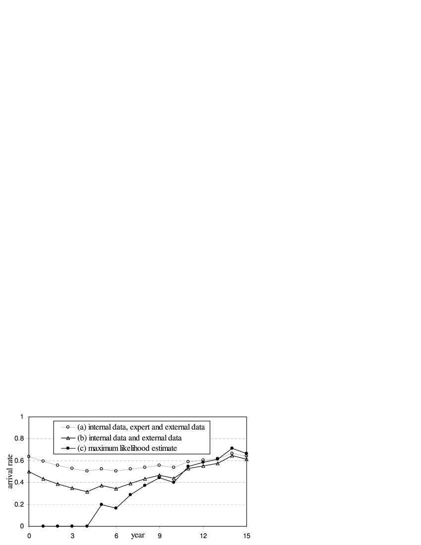
Figure 3: Three estimators for the Poisson arrival rate vs the observation year: (a) Bayesian estimator combining internal data, expert opinion $\hat{\vartheta}=0.7$ and external data; (b) Bayesian estimator combining internal data and external data; (c) MLE based on internal data only. The internal data annual counts (0,0,0,0,1,0,1,1,1,0,2,1,1,2,0) were sampled from the $Poisson(0.6)$. The prior implied by external data is $Gamma(\alpha,\beta)$ with $\rm{mean}=0.5$.

Example. Suppose that the annual frequency $N$ is modeled by a Poisson distribution $Poisson(\lambda)$ and the prior $\pi(\lambda)$ for $\lambda$ is $Gamma(\alpha,\beta)$. As described above, the prior can be estimated using either expert opinions or external data. The expert may specify the “best” estimate for the expected number of events $E[E[N|\lambda]]=E[\lambda]$ and an uncertainty that the “true” $\lambda$ for next year is within the interval [$a$,$b$] with the probability $\Pr[a\leq\lambda\leq b]=p$. Then the equations $E[\lambda]=\alpha\beta$ and $p=\int_{a}^{b}{\pi(\lambda)d\lambda}$ can be solved numerically to estimate the structural parameters $\alpha$ and $\beta$. In the insurance industry, the uncertainty for the “true” $\lambda$ is often measured in terms of the coefficient of variation, $\rm{Vco}(\lambda)=\sqrt{\rm{var}(\lambda)}/E[\lambda]$. Given the estimates for $E[\lambda]=\alpha\beta$ and $\rm{Vco}(\lambda)=1/\sqrt{\alpha},$ the structural parameters $\alpha$ and $\beta$ are easily estimated. For example, if the expert specifies (or external data imply) that $E[\lambda]=0.5$ and $\Pr[0.25\leq\lambda\leq 0.75]=2/3,$ then we can fit a prior $Gamma(\alpha\approx 3.407,\beta\approx 0.147)$. This prior is used in Figure 3, presenting the posterior best estimate for the arrival rate calculated using (34) and referred to as estimator (b), when the annual counts data $N(k)$, $k=1,\ldots,15$ are simulated from $Poisson(0.6)$. Note that, in Figure 3, the prior is considered to be implied by external data. On the same Figure we show the standard MLE, $\hat{\lambda}_{{}^{k}}^{MLE}=\frac{1}{k}\sum\nolimits_{i=1}^{k}{n(i)}$, referred to as estimator (c). For a small number of observed years the Bayesian estimator (b) is more accurate as it takes prior information into account. For a large sample size, both the MLE and Bayesian estimators converge to the true value 0.6. Also, the Bayesian estimator is more stable (smooth) with respect to bad years. The same behavior is observed if the experiment is repeated many times with different sequences of random numbers. This and other examples can be found in [47].

7.3 Combining three data sources

In Section 7.1, Bayesian inference was used to combine two data sources, i.e. expert opinion with internal data, or external data with internal data. An approach to combine all three data sources (internal data, expert opinion and external data) can be accomplished as described in Lambrigger et al. [51]. Consider data ${\rm{\bf X}}$ and expert opinions ${{\bm{\upsilon}}}$ on parameter ${{\bm{\theta}}}$. Then the posterior is

$$\pi({{\bm{\theta}}}|{\rm{\bf x}},{{\bm{\upsilon}}})\propto\ell_{1}({\rm{\bf x}}|{{\bm{\theta}}})\ell_{2}({{\bm{\upsilon}}}|{{\bm{\theta}}})\pi({{\bm{\theta}}}),$$ (36)

where $\ell_{1}({\rm{\bf x}}|{{\bm{\theta}}})$ is the likelihood of data given ${{\bm{\theta}}}$, $\ell_{2}({{\bm{\upsilon}}}|{{\bm{\theta}}})$ is the likelihood of expert opinions and $\pi({{\bm{\theta}}})$ is the prior density estimated using external data. This posterior for ${{\bm{\theta}}}$ combines information from internal data, expert opinions and external data. Here it is assumed that given ${{\bm{\theta}}}$, expert opinions are independent from internal data. A more general relation $\pi({{\bm{\theta}}}|{\rm{\bf x}},{{\bm{\upsilon}}})\propto\ell({\rm{\bf x}},{{\bm{\upsilon}}}|{{\bm{\theta}}})\pi({{\bm{\theta}}})$ can be considered to avoid this assumption.

For illustration purposes, consider modeling of the annual counts: assume that the annual counts $N(1),\ldots,N(T)$ are iid from $Poisson(\lambda)$; expert opinions $\upsilon_{1},\ldots,\upsilon_{M}$ on $\lambda$ are iid from $Gamma(\xi,\lambda/\xi)$; and the prior on $\lambda$ is $Gamma(\alpha,\beta)$. Then the posterior is the generalized inverse gamma density

$$\pi(\lambda|{\rm{\bf n}},{{\bm{\upsilon}}}) \propto \pi(\lambda)\ell({\rm{\bf n}}|\lambda)\ell({{\bm{\upsilon}}}|\lambda)$$

$$\propto \lambda^{\alpha-1}e^{-\lambda/\beta}\prod\limits_{t=1}^{T}{e^{-\lambda}\frac{\lambda^{n(t)}}{n(t)!}}\prod\limits_{m=1}^{M}{e^{-\upsilon_{m}\xi/\lambda}\frac{\upsilon_{m}^{\xi-1}}{(\lambda/\xi)^{\xi}}}\propto\lambda^{{\kern 1.0pt}\nu}e^{-\lambda\omega-\phi/\lambda},$$

$$\nu = \alpha-1+\sum\limits_{t=1}^{T}{n(t)}-M\xi,\quad\omega=T+1/\beta,\quad\phi=\xi\sum\limits_{m=1}^{M}{\upsilon_{m}}.$$ (37)

In Figure 3, we show the posterior best estimate for the arrival rate $E[\lambda|{\rm{\bf N}},{{\bm{\upsilon}}}]$ combining three data sources (referred to as estimator (a)) and compare it with the estimator $E[\lambda|{\rm{\bf N}}]$ combining internal and external data (referred to as estimator (b), also see (21)). The counts $N(k)$, $k=1,\ldots,15$ are simulated from $Poisson(0.6)$; the assumed prior distribution implied by external data is the same as considered in the example in Section 7.2, i.e. $Gamma(\alpha\approx 3.41,\;\beta\approx 0.15)$ such that $E[\lambda]=0.5$ and $\Pr[0.25\leq\lambda\leq 0.75]=2/3$; and there is one expert opinion $\hat{\upsilon}=0.7$ from the distribution with ${\rm{Vco}}(\upsilon|\lambda)=$0.5, i.e $\xi=4$. The standard maximum likelihood estimate of the arrival rate $\lambda_{k}^{MLE}=\frac{1}{k}\sum\nolimits_{i=1}^{k}{n(i)}$ is referred to as estimator (c). Estimator (a), combining all three data sources, certainly outperforms other estimators and is more stable around the true value, especially for small data sample size. All estimators converge to the true value as the number of observed years increases. The same behavior is observed if the experiment is repeated; see detailed discussions in [51].

8 Modeling dependence

Basel II requires (see [1, p.152]) that: “Risk measures for different operational risk estimates must be added for purposes of calculating the regulatory minimum capital requirement. However, the bank may be permitted to use internally determined correlations in operational risk losses across individual operational risk estimates, provided it can demonstrate to the satisfaction of the national supervisor that its systems for determining correlations are sound, implemented with integrity, and take into account the uncertainty surrounding any such correlation estimates (particularly in periods of stress). The bank must validate its correlation assumptions using appropriate quantitative and qualitative techniques”. Thus if dependence is properly quantified between all risk cells $j=1,\ldots,J$ then, under the LDA model (1), the capital is calculated as

$$VaR_{0.999}\left({Z_{(\bullet)}(T+1)=\sum\limits_{j=1}^{J}{Z_{j}(T+1)}}\right),$$ (38)

otherwise the capital should be estimated as

$$\sum\limits_{j=1}^{J}{VaR_{0.999}\left({Z_{j}(T+1)}\right)}.$$ (39)

Adding up VaRs for capital estimation is equivalent to an assumption of perfect positive dependence between the annual losses $Z_{j}(T+1)$, $j=1,\ldots,J$. In principle, VaR can be estimated at any level of granularity and then the capital is calculated as a sum of resulting VaRs. Often banks quantify VaR for business lines and add up these estimates to get capital, but for simplicity of notations, (39) is given at the level of risk cells. It is expected that the capital under (38) is less than (39); 20% diversification is not uncommon. However, it is important to note that VaR is not a coherent risk measure, see Artzner et al. [52]. In particular, under some circumstances VaR measure may fail a sub-additivity property

$$VaR_{q}(Z_{(\bullet)}(T+1))\leq\sum\limits_{j=1}^{J}{VaR_{q}(Z_{j}(T+1)}),$$ (40)

see Embrechts et al. [53] and [54], i.e. dependence modeling could also increase VaR. As can be seen from the literature, the dependence between different ORs can be introduced by:

• Modeling dependence between the annual counts via a copula, as described in Frachot et al. [55], Bee [56], Aue and Klakbrener [10];

• Using common shock models to introduce events common across different risks and leading to the dependence between frequencies studied in Lindskog and McNeil [57] and Powojowski et al. [58]. Dependence between severities occurring at the same time is considered in Lindskog and McNeil [57];

• Modeling dependence between the $k$th severities or between $k$th event times of different risks; see Chavez-Demoulin et al. [8] (e.g. $1^{st}$, $2^{nd}$, etc losses/event times of the $j$th risk are correlated to the $1^{st}$, $2^{nd}$, etc losses/event times of the $i$th risk respectively);

• Modeling dependence between the annual losses of different risks via copulas; see Giacometti et al. [59], Embrechts and Puccetti [60];

• Using the multivariate compound Poisson model based on Lévy copulas suggested in Böcker and Klüppelberg [61], [62];

• Using structural models with common (systematic) factors that can lead to the dependence between severities and frequencies of different risks and within risk;

• Modeling dependence between severities and frequencies from different risks and within risk using dependence between risk profiles considered in Peters et al. [44].

Below, we describe the main concepts involved into these approaches.

8.1 Copula

The concept of a copula is a flexible and general technique to model dependence; for an introduction see e.g. Joe [63] and Nelson [64]; and for application in financial risk management see e.g. [6, Section 5]. In brief, a copula is a $d$-dimensional multivariate distribution on $[0,1]^{d}$ with uniform margins. Given a copula function $C$(.) and univariate marginal distributions $F_{1}(.),\ldots,F_{d}(.)$, the joint distribution with these margins can be constructed as

$$F(x_{1},\ldots,x_{d}))=C(F_{1}(x_{1}),\ldots,F_{d}(x_{d})).$$ (41)

A well known theorem due to Sklar, published in 1959, says that one can always find a unique copula $C$(.) for a joint distribution with given continuous margins. In the case of discrete distributions this copula may not be unique. The most commonly used copula (due its simple calibration and simulation) is the Gaussian copula, implied by the multivariate Normal distribution. It is a distribution of $U_{1}=F_{N}(X_{1}),\ldots,U_{d}=F_{N}(X_{d})$, where $F_{N}(.)$ is the standard Normal distribution and $X_{1},\ldots,X_{d}$ are from the multivariate Normal distribution $F_{\Sigma}($.) with zero mean, unit variances and correlation matrix $\Sigma$. Formally, in explicit form, the Gaussian copula is

$$C_{\Sigma}^{Ga}(u_{1},\ldots,u_{n})=F_{\Sigma}(F_{N}^{-1}(u_{1}),\ldots,F_{N}^{-1}(u_{d})).$$ (42)

There are many other copulas (e.g. t-copula, Clayton copula, Gumbel copulas to mention a few) studied in academic research and used in practice, that can be found in the referenced literature.

8.2 Dependence between frequencies via copula

The most popular approach in practice is to consider a dependence between the annual counts of different risks via a copula. Assuming a $J$-dimensional copula $C(.)$ and the marginal distributions $P_{j}(.)$ for the annual counts $N_{1}(t),\ldots,N_{J}(t)$ leads to a model

$$N_{1}(t)=P_{1}^{-1}(U_{1}(t)),\ldots,N_{J}(t)=P_{J}^{-1}(U_{J}(t)),$$ (43)

where $U_{1}(t),\ldots,U_{J}(t)$ are uniform (0,1) rvs from a copula $C(.)$ and $P_{j}^{-1}(.)$ is the inverse marginal distribution of the counts in the $j$th risk. Here, $t$ is a discrete time (typically in annual units but shorter steps might be needed to calibrate the model) and usually the counts are assumed to be independent between different $t$ steps. The approach allows us to model both positive and negative dependence between counts. As reported in the literature, the implied dependence between annual losses even for a perfect dependence between counts is relatively small and as a result the impact on capital is small too. Some theoretical reasons for the observation that frequency dependence has only little impact on the operational risk capital charge are given in [61]. As an example, in Figure 4 we plot Spearman’s rank correlation between the annual losses of two risks, $Z_{1}$ and $Z_{2}$, induced by the Gaussian copula dependence between frequencies. Marginally, the frequencies $N_{1}$ and $N_{2}$ are from the Poisson distributions with the intensities $\lambda=5$ and $\lambda=10$ respectively and the severities are from $LN(\mu=1,\sigma=2)$ distributions for both risks.

8.3 Dependence between aggregated losses via copula

Dependence between the aggregated losses can be introduced similarly to (43). In this approach, one can model the aggregated losses as

$$Z_{1}(t)=F_{1}^{-1}(U_{1}(t)),\ldots,Z_{J}(t)=F_{J}^{-1}(U_{J}(t)),$$ (44)

where $U_{1}(t),\ldots,U_{J}(t)$ are uniform (0,1) rvs from a copula $C(.)$ and $F_{j}^{-1}(.)$ is the inverse marginal distribution of the aggregated loss of the $j$-th risk. Note that the marginal distribution $F_{j}(.)$ should be calculated using frequency and severity distributions. Typically, the data are available over several years only and a short time step $t$ (e.g. quarterly) is needed to calibrate the model. This dependence modeling approach is probably the most flexible in terms of the range of achievable dependencies between risks; e.g. perfect positive dependence between the annual losses is achievable. However, note that this approach may create difficulties with incorporation of insurance into the overall model. This is because an insurance policy may apply to several risks with the cover limit applied to the aggregated loss recovery; see Section 9.

8.4 Dependence between the kth event times/losses

Theoretically, one can introduce dependence between the $k$th severities or between the $k$th event inter-arrival times or between the $k$th event times of different risks. For example: $1^{st}$, $2^{nd}$, etc losses of the$j$th risk are correlated to the $1^{st}$, $2^{nd}$, etc losses of the $i$th risk respectively while the severities within each risk are independent. The actual dependence can be done via a copula similar to (43), for an accurate description we refer to [8]. Here, we would like to note that a physical interpretation of such models can be difficult. Also, an example of dependence between annual losses induced by dependence between the $k$th inter-arrival times is presented in Figure 4.

8.5 Modeling dependence via Lévy copulas

Böcker and Klüppelberg [61, 62] suggested to model dependence in frequency and severity between different risks at the same time using a new concept of Lévy copulas, see e.g. [65, Sections 5.4-5.7]. It is assumed that each risk follows to a univariate compound Poisson process (that belongs to a class of Lévy processes). Then, the idea is to introduce the dependence between risks in such a way that any conjunction of different risks constitutes a univariate compound Poisson process. It is achieved using the multivariate compound Poisson processes based on Lévy copulas. Note that, if dependence between frequencies or annual losses is introduced via copula as in (43) or (44), then the conjunction of risks does not follow to a univariate compound Poisson.

The precise definitions of Lévy measure and Lévy copula are beyond the purpose of this paper and can be found in the above mentioned literature. Here, we would like to mention that in the case of a compound Poisson process Lévy measure is the expected number of losses per unit of time with a loss amount in a pre-specified interval, $\bar{\Pi}_{j}(x)=\lambda_{j}\Pr(X_{j}>x)$. Then the multivariate Lévy measure can be constructed from the marginal measures and a Lévy copula $\tilde{C}$ as

$$\bar{\Pi}(x_{1},\ldots,x_{d})=\tilde{C}(\bar{\Pi}_{1}(x_{1}),\ldots,\bar{\Pi}_{d}(x_{d}))$$ (45)

which is somewhat similar to (41) in a sense that the dependence structure between different risks can be separated from the marginal processes. However, it is quite a different concept. In particular, a Lévy copula for processes with positive jumps is $[0,\infty)^{d}\to[0,\infty)$ mapping while a standard copula (41) is $[0,1]^{d}\to[0,1]$ mapping. Also, a Lévy copula controls dependence between frequencies and dependence between severities (from different risks) at the same time. The interpretation of this model is that dependence between different risks is due to the loss events occurring at the same time. Important implication of this approach is that a total bank’s loss can be modeled as a compound Poisson process with some intensity and iid severities. If this common severity distribution is sub-exponential then closed-form approximation (23) can be used to estimate VaR of the total annual loss in a bank.

8.6 Structural model with common factors

The use of common (systematic) factors is useful to identify dependent risks and to reduce the number of required correlation coefficients that must be estimated, see e.g. [6, Section 3.4]. Structural models with common factors to model dependence are widely used in credit risk, see industry examples in [6, Section 8.3.3]. For OR, these models are qualitatively discussed in Marshall [66, Sections 5.3 and 7.4] and there are unpublished examples of a practical implementation. As an example, assume a Gaussian copula for the annual counts of different risks and consider one common (systematic) factor $\Omega(t)$ affecting the counts as follows:

$$Y_{j}(t) = \rho_{j}\Omega(t)+\sqrt{1-\rho_{j}^{2}}W_{j}(t),\quad j=1,\ldots,J;\quad$$

$$N_{1}(t) = P_{1}^{-1}\left({F_{N}(Y_{1}(t))}\right),\ldots,N_{J}(t)=P_{J}^{-1}\left({F_{N}(Y_{J}(t))}\right).$$ (46)

Here, $W_{1}(t),\ldots,W_{J}(t)$ and $\Omega(t)$ are independent rvs from the standard Normal distribution. All rvs are independent between different time steps $t$. Given $\Omega(t)$, the counts are independent but unconditionally the risk profiles are dependent if the corresponding $\rho_{j}$ are nonzero. In this example, one should identify $J$ correlation parameters $\rho_{j}$ only instead of $J(J-1)/2$ parameters of the full correlation matrix.

Extension of this approach to many factors $\Omega_{k}(t)$, $k=1,\ldots,K$ is easy:

$$Y_{j}(t)=\sum\limits_{k=1}^{K}{\rho_{jk}\Omega_{k}(t)}+\sqrt{1-\sum\limits_{k=1}^{K}{\rho_{jk}\rho_{jm}{\rm{cov}}(\Omega_{k}(t)\Omega_{m}(t))}}W_{j}(t),$$ (47)

where $\Omega_{1}(t),\ldots,\Omega_{K}(t)$ are from a multivariate Normal distribution with zero means, unit variances and some correlation matrix. This approach can also be extended to introduce a dependence between both severities and frequencies. For example, in the case of one factor, one can structure the model as follows:

$$Y_{j}(t) = \rho_{j}\Omega(t)+\sqrt{1-\rho_{j}^{2}}W_{j}(t),\quad j=1,\ldots,J;$$

$$N_{j}(t) = P_{j}^{-1}\left({F_{N}(Y_{j}(t))}\right),\quad j=1,\ldots,J;$$

$$R_{j}^{(s)}(t) = \tilde{\rho}_{j}\Omega(t)+\sqrt{1-\tilde{\rho}_{j}^{2}}V_{j}^{(s)}(t),\quad s=1,\ldots,N_{j}(t),\quad j=1,\ldots,J;$$

$$X_{j}^{(s)}(t) = F_{j}^{-1}\left({F_{N}(R_{j}^{(s)}(t))}\right),\quad s=1,\ldots,N_{j}(t),\quad j=1,\ldots,J.$$

Here: $W_{j}(t)$, $V_{j}^{(s)}(t)$, $s=1,\ldots,N_{j}(t)$, $j=1,\ldots,J$ and $\Omega(t)$ are iid from the standard Normal distribution. Again, the logic is that there is a factor affecting severities and frequencies within a year such that conditional on this factor, severities and frequencies are independent. The factor is changing stochastically from year to year, so that unconditionally there is dependence between frequencies and severities. Also note that in such setup, there is a dependence between severities within a risk category. Often, common factors are unobservable and practitioners use generic intuitive definitions such as: changes in political, legal and regulatory environments, economy, technology, system security, system automation, etc. Several external and internal factors are typically considered, so that some of the factors affect frequencies only (e.g. system automation), some factors affect severities only (e.g. changes in legal environment) and some factors affect both the frequencies and severities (e.g. system security).

8.7 Stochastic and dependent risk profiles

Consider the LDA for risk cells $j=1,\ldots,J$:

$$Z_{j}(t)=\sum\limits_{s=1}^{N_{j}(t)}{X_{j}^{(s)}(t)},\quad t=\mbox{1,2,\ldots}\quad,$$ (48)

where $N_{j}(t)\sim P_{j}(.|\lambda_{t}^{(j)})$ and $X_{j}^{(s)}(t)\sim F_{j}(.|\psi_{t}^{(j)})$. Hereafter, notation $X\sim F(.)$ means that $X$ is a rv from distribution $F(.)$. It is realistic to consider that the risk profiles ${{\bm{\lambda}}}_{t}=(\lambda_{t}^{(1)},\ldots,\lambda_{t}^{(J)})$ and ${{\bm{\psi}}}_{t}=(\psi_{t}^{(1)},\ldots,\psi_{t}^{(J)})$ are not constant but changing in time stochastically due to changing risk factors (e.g. changes business environment, politics, regulations, etc). Also it is realistic to say that risk factors affect many risk cells and thus the risk profiles are dependent. One can model this by assuming some copula $C(.)$ and marginal distributions for the risk profiles (also see [67]), i.e. the joint distribution between the risk profiles is

$$F\left({{{\bm{\lambda}}}(t),{{\bm{\psi}}}(t)}\right)=C\left({G_{1}(\lambda_{1}(t)),\ldots,G_{J}(\lambda_{J}(t)),H_{1}(\psi_{1}(t)),\ldots,H_{J}(\psi_{J}(t))}\right),$$ (49)

where $G_{j}(.)$ and $H_{j}(.)$ are the marginal distributions of $\lambda_{j}(t)$ and $\psi_{j}(t)$ respectively. Dependence between the risk profiles will induce a dependence between the annual losses. This general model can be used to model dependence between the annual counts; between the severities of different risks; between the severities within a risk; and between the frequencies and severities. The likelihood of data (counts and severities) can be derived but involves a multidimensional integral with respect to latent variables (risk profiles). Advanced MCMC methods (such as the Slice Sampler method used in [67]) can be used to fit the model. For example, consider the bivariate case ($J=2)$ where:

• Frequencies $N_{j}(t)\sim Poisson(\lambda_{j}(t))$ and severities $X_{j}^{(s)}(t)\sim LN(\mu_{j}(t),\sigma_{j}(t))$;

• $\lambda_{1}(t)\sim Gamma(2.5,2)$, $\lambda_{2}(t)\sim Gamma(5,2)$, $\mu_{j}(t)\sim Normal(1,1)$, $\sigma_{j}(t)=2;$

• The dependence between $\lambda_{1}(t)$, $\lambda_{2}(t)$, $\mu_{1}(t)$ and $\mu_{2}(t)$ is a Gaussian copula.

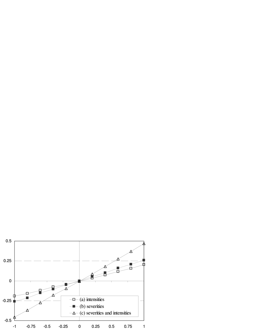
Figure 5: Spearman’s rank correlation $\rho_{S}(Z_{1},Z_{2})$ between annual losses vs the Gaussian copula parameter $\rho$: (a) – copula for the frequency profiles $\lambda_{1}$ and $\lambda_{2}$; (b) – copula for the severity profiles $\mu_{1}$ and $\mu_{2}$; (c) – copula for $\lambda_{1}$ and $\lambda_{2}$ and the same copula for $\mu_{1}$ and $\mu_{2}$

Figure 5 shows the induced dependence between the annual losses $Z_{1}(t)$ and $Z_{2}(t)$ vs the copula dependence parameter for three cases: if only $\lambda_{1}(t)$ and $\lambda_{2}(t)$ are dependent; if only $\mu_{1}(t)$ and $\mu_{2}(t)$ are dependent; if the dependence between $\lambda_{1}(t)$ and $\lambda_{2}(t)$ is the same as between $\mu_{1}(t)$ and $\mu_{2}(t)$. In all cases the dependence is Gaussian copula.

8.8 Common shock processes

Modeling OR events affecting many risk cells can be done using common shock process models; see Johnson et al. [68, Section 37]. In particular, consider $J$ risks with the event counts $N_{j}(t)=N^{(C)}(t)+\tilde{N}_{j}(t)$, where $\tilde{N}_{j}(t)$, $j=1,\ldots,J$ and $N^{(C)}(t)$ are generated by independent Poisson processes with intensities $\tilde{\lambda}_{j}$ and $\lambda_{C}$ respectively. Then $N_{j}(t)$, $j=1,\ldots,J$ are Poisson distributed with intensities $\lambda_{j}=\tilde{\lambda}_{j}+\lambda_{C}$ marginally and are dependent via the common events $N^{(C)}(t)$. The linear correlation and covariance between risk counts are $\rho(N_{i}(t),N_{j}(t))=\lambda_{C}/\sqrt{\lambda_{i}\lambda_{j}}$ and ${\rm{cov}}(N_{i}(t),N_{j}(t))=\lambda_{C}$ respectively. Only a positive dependence between counts can be modeled using this approach. Also, note that the covariance for any pair of risks is the same though the correlations are different. More flexible dependence can be achieved by allowing a common shock process to contribute to the $k$-th risk process with some probability $p_{k}$; then ${\rm{cov}}(N_{i}(t),N_{j}(t))=\lambda_{C}p_{i}p_{j}$. This method can be generalized to many common shock processes; see [57] and [58]. It is also reasonable to consider the dependence between the severities in different risk cells that occurred due to the same common shock event.

9 Insurance

Many ORs are insured. If a loss occurred and it is covered by an insurance policy then part of the loss will be recovered. A typical policy will provide a recovery $R$ for a loss $X$ subject to the excess amount (deductible) $D$ and top cover limit amount $U$ as follows:

$$R=\left\{{{\begin{array}[]{*{20}c}{0,\quad\mbox{if }0\leq X<D;\hfill}\\ {X-D,\quad\mbox{if }D\leq X<U+D;\hfill}\\ {U,\quad\mbox{if }D+U\leq X.\hfill}\\ \end{array}}}\right.$$ (50)

That is the recovery will take place if the loss is larger than the excess and the maximum recovery that can be obtained from the policy is $U$. Note that in (50), the time of the event is not involved and the top cover limit applies for a recovery per risk event, i.e. for each event the obtained recovery is subject of the top cover limit. Including insurance into the LDA is simple; the loss severity in (1) should be simply reduced by the amount of recovery (50) and can be viewed as a simple transformation of the severity. However, there are several difficulties in practice. Policies may cover several different risks and different policies may cover the same risk. The top cover limit may apply for the aggregated recovery over many events of one or several risks (e.g. the policy will pay the recovery for losses until the top cover limit is reached by accumulated recovery). These aspects and special insurance haircuts required by Basel II [1] make recovery dependent on time. Accurate modeling insurance accounting for practical details requires modeling the event times rather than the annual counts only, e.g. a Poisson process can be used to model the event times. It is not difficult to incorporate the insurance into an overall model if a Monte Carlo method is used to quantify the annual loss distributions.

The Basel II requires that the total capital reduction due to the insurance recoveries is capped by 20%. Incorporating insurance into the LDA is not only important for capital reduction but also beneficial for negotiating a fair premium with the insurer because the distribution of the recoveries and its characteristics can be estimated.

10 Capital charge via full predictive distribution

Consider the annual loss in a bank (or the annual loss at a different level depending on where the 0.999 quantiles are quantified; see Section 8) over the next year, $Z(T+1)$. Denote the density of the annual loss, conditional on parameters ${{\bm{\theta}}}$, as $f(z(T+1)|{{\bm{\theta}}})$. Typically, given observations, the MLEs ${{\hat{\bm{\theta}}}}$ are used as the “best fit” point estimators for ${{\bm{\theta}}}$. Then the annual loss distribution for the next year is estimated as $f(z(T+1)|{{\hat{\bm{\theta}}}})$ and its 0.999 quantile, $Q_{0.999}({{\hat{\bm{\theta}}}})$, is used for the capital charge calculation.

However, the parameters ${{\bm{\theta}}}$ are unknown and it is important to account for this uncertainty when capital charge is estimated (especially for risks with small datasets) as discussed in [69]. If Bayesian inference is used to quantify the parameters through their posterior distribution $\pi({{\bm{\theta}}}|{\rm{\bf y}})$, then the full predictive density (accounting for parameter uncertainty) of $Z(T+1)$, given all data ${\rm{\bf Y}}$ used in the estimation procedure, is

$$f(z(T+1)|{\rm{\bf y}})=\int{f(z(T+1)|{{\bm{\theta}}})\times\pi({{\bm{\theta}}}|{\rm{\bf y}})d{{\bm{\theta}}}}.$$ (51)

Here, it is assume that, given parameters ${{\bm{\theta}}}$, $Z(T+1)$ and ${\rm{\bf Y}}$ are independent. If a frequentist approach is taken to estimate the parameters, then ${{\bm{\theta}}}$ should be replaced with ${{\hat{\bm{\theta}}}}$ and the integration should be done with respect to the density of parameter estimators ${{\hat{\bm{\theta}}}}$. The 0.999 quantile of the full predictive distribution (51),

$$Q_{q}^{B}=F_{Z(T+1)|{\rm{\bf Y}}}^{-1}(q)=\inf\{z:\Pr[Z(T+1)>z|{\rm{\bf Y}}]\leq 1-q\},\;q=0.999,$$ (52)

can be used as a risk measure for capital calculations.

Another approach under a Bayesian framework to account for parameter uncertainty is to consider a quantile $Q_{0.999}({{\bm{\theta}}})$ of the conditional annual loss density $f(.|{{\bm{\theta}}})$:

$$Q_{q}({{\bm{\theta}}})=F_{Z(T+1)|{{\bm{\theta}}}}^{-1}(q)=\inf\{z:\Pr[Z(T+1)>z|{{\bm{\theta}}}]\leq 1-q\},\;q=0.999.$$ (53)

Then, given that ${{\bm{\theta}}}$ is distributed as $\pi({{\bm{\theta}}}|{\rm{\bf y}})$, one can find the distribution of $Q_{0.999}({{\bm{\theta}}})$ and form a predictive interval to contain the true value with some probability. This is similar to forming a confidence interval in the frequentist approach using the distribution of $Q_{0.999}({{\hat{\bm{\theta}}}})$, where ${{\hat{\bm{\theta}}}}$ is treated as random (usually, the Gaussian approximation (24) is assumed for ${{\hat{\bm{\theta}}}})$. Often, if derivatives can be calculated efficiently, the variance of $Q_{0.999}({{\hat{\bm{\theta}}}})$ is simply estimated via an error propagation method and a first order Taylor expansion). Here, one can use deterministic algorithms such as FFT or Panjer recursion to calculate $Q_{0.999}({{\bm{\theta}}})$ efficiently. Under this approach, one can argue that the conservative estimate of the capital charge accounting for parameter uncertainty should be based on the upper bound of the constructed interval. Note that specification of the confidence level is required and it might be difficult to argue that the commonly used confidence level $0.95$ is good enough for estimation of the 0.999 quantile.

In OR, it seems that the objective should be to estimate the full predictive distribution (51) for the annual loss $Z(T+1)$ over next year conditional on all available information and then estimate the capital charge as a quantile $Q_{0.999}^{B}$ of this distribution (52.

Consider a risk cell in the bank. Assume that the frequency $p(.|{{\bm{\alpha}}})$ and severity $f(.|{{\bm{\beta}}})$ densities for the cell are chosen. Also, suppose that the posterior distribution $\pi({{\bm{\theta}}}|{\rm{\bf y}})$, ${{\bm{\theta}}}=({{\bm{\alpha}}},{{\bm{\beta}}})$ is estimated. Then, the full predictive annual loss distribution (51) in the cell can be calculated using Monte Carlo procedure with the following logical steps:

1. For $k=1,\ldots,K$

   1. For a given risk simulate the risk parameters ${{\bm{\theta}}}=({{\bm{\alpha}}},{{\bm{\beta}}})$ from the posterior $\pi({{\bm{\theta}}}|{\rm{\bf y}})$. If the posterior is not known in closed form then this simulation can be done using MCMC (see Section 6.2). For example, one can run MCMC for $K$ iterations beforehand and simply take the $k$th iteration parameter values.

   2. Given ${{\bm{\theta}}}=({{\bm{\alpha}}},{{\bm{\beta}}})$, simulate the annual number of events $N$ from $p(.|{{\bm{\alpha}}})$ and severities $X^{(1)},\ldots,X^{(N)}$ from $f(.|{{\bm{\beta}}})$; and calculate the annual loss $Z^{(k)}=\sum\nolimits_{n=1}^{N}{X^{(n)}}$.

2. Next $k$

Obtained annual losses $Z^{(1)},\ldots,Z^{(K)}$ are samples from the full predictive density (51). Extending the above procedure to the case of many risks is easy but requires specification of the dependence model, see Section 8. In this case, in general, all model parameters (including the dependence parameters) should be simulated from their joint posterior in Step 1. Then, given these parameters, Step 2 should simulate all risks with a chosen dependence structure. In general, sampling from the joint posterior of all model parameters can be accomplished via MCMC, see e.g. [67, 70]. The 0.999 quantile $Q_{0.999}^{B}$ and other distribution characteristics can be estimated using the simulated samples in the usual way, see Section 5.1.

Note that in the above Monte Carlo procedure the risk profiles ${{\bm{\alpha}}}$ and ${{\bm{\beta}}}$ are simulated from their posterior distribution for each simulation. Thus, we model both the process risk (process uncertainty), which comes from the fact that frequencies and severities are rvs, and the parameter risk (parameter uncertainty), which comes from the fact that we do not know the true values of ${{\bm{\theta}}}=({{\bm{\alpha}}},{{\bm{\beta}}})$. To calculate the conditional density $f(z|{\rm{\hat{\bm{\theta}}}})$ and its quantile $Q_{0.999}({{\hat{\bm{\theta}}}})$ using parameter point estimators ${{\hat{\bm{\theta}}}}$, step 1 in the above procedure should be simply modified by setting ${{\bm{\theta}}}={{\hat{\bm{\theta}}}}$ for all simulations $k=1,\ldots,K$. Thus, Monte Carlo calculations of $Q_{0.999}^{B}$ and $Q_{0.999}({{\hat{\bm{\theta}}}})$ are similar, given that $\pi({{\bm{\theta}}}|{\rm{\bf y}})$ is known. If $\pi({{\bm{\theta}}}|{\rm{\bf y}})$ is not known in closed form then it can be estimated efficiently using Gaussian approximation or available MCMC algorithms; see Section 6.2.

The parameter uncertainty is ignored by the estimator $Q_{0.999}({\hat{\bm{\theta}}})$ but is taken into account by $Q_{0.999}^{B}$. Figure 6 presents results for the relative bias (averaged over 100 realizations) $E[Q_{0.999}^{B}-Q_{0.999}({{\hat{\bm{\theta}}}})]/Q^{(0)}$, where ${{\hat{\bm{\theta}}}}$ is MLE, $Q^{(0)}$ is the quantile of $f(.|{{\bm{\theta}}}_{0})$ and ${{\bm{\theta}}}_{0}$ is the true value of the parameter. The frequencies and severities are simulated from $Poisson(\lambda_{0}=10)$ and $LN(\mu_{0}=1,\sigma_{0}=2)$ respectively. Also, constant priors are used for the parameters so that there are closed form expressions for the posterior. In this example, the bias induced by parameter uncertainty is large: it is approximately 10% after 40 years (i.e. approximately 400 data points) and converges to zero as the number of losses increases.

The parameter values used in the example may not be typical for some ORs. One should do the above analysis with real data to find the impact of parameter uncertainty. For example a similar analysis for a multivariate case was performed in [70] with real data. For high frequency low impact risks, where a large amount of data is available, the impact is certainly expected to be small. However for low frequency high impact risks, where the data are very limited, the impact can be significant. Also, see Mignola and Ugoccioni [71] for discussion of uncertainties involved in OR estimation.

11 Conclusions

In this paper we reviewed some methods suggested in the literature for the LDA implementation. We emphasized that Bayesian methods can be well suited for modeling OR. In particular, Bayesian framework is convenient to combine different data sources (internal data, external data and expert opinions) and to account for the relevant uncertainties. Accurate quantification of the dependences between ORs is a difficult task with many challenges to be resolved. There are many aspects of the LDA that may require sophisticated statistical methods and different approaches are hotly debated.

12 Acknowledgments

The author would like to thank Mario Wüthrich, Hans Bühlmann, Gareth Peters, Xiaolin Luo, John Donnelly and Mark Westcott for fruitful discussions, useful comments and encouragement. Also, the comments from anonymous referee helped to improve the paper.

Basel II business lines (BL)	Basel II event types (ET)
• Corporate finance ($\beta_{1}=0.18$) • Trading & Sales ($\beta_{2}=0.18$) • Retail banking ($\beta_{3}=0.12$) • Commercial banking ($\beta_{4}=0.15$) • Payment & Settlement ($\beta_{5}=0.18$) • Agency Services ($\beta_{6}=0.15$) • Asset management ($\beta_{7}=0.12$) • Retail brokerage ($\beta_{8}=0.12$)	• Internal fraud • External fraud • Employment practices and workplace safety • Clients, products and business practices • Damage to physical assets • Business disruption and system failures • Execution, delivery and process management

Table 1: Basel II business lines and event types. $\beta_{1},\ldots,\beta_{8}$ are the business line factors used in the Basel II Standardised Approach.

Figure 1: Relative bias in the 0.999 quantile of the annual loss vs % of truncated points for several models ignoring truncation in the case of light tail severities from $LN(3,1)$. The annual counts above the truncation level are from $Poisson(10)$.

Figure 4: Spearman’s rank correlation between the annual losses $\rho_{S}(Z_{1},Z_{2})$ vs the Gaussian copula parameter $\rho$: (a) – copula between counts $N_{1}$ and $N_{2}$; (b) – copula between inter-arrival times of two Poisson processes. Marginally, the frequencies are from $Poisson(5)$ and $Poisson(10)$ respectively and the severities are iid from $LN(1,2)$ for both risks.

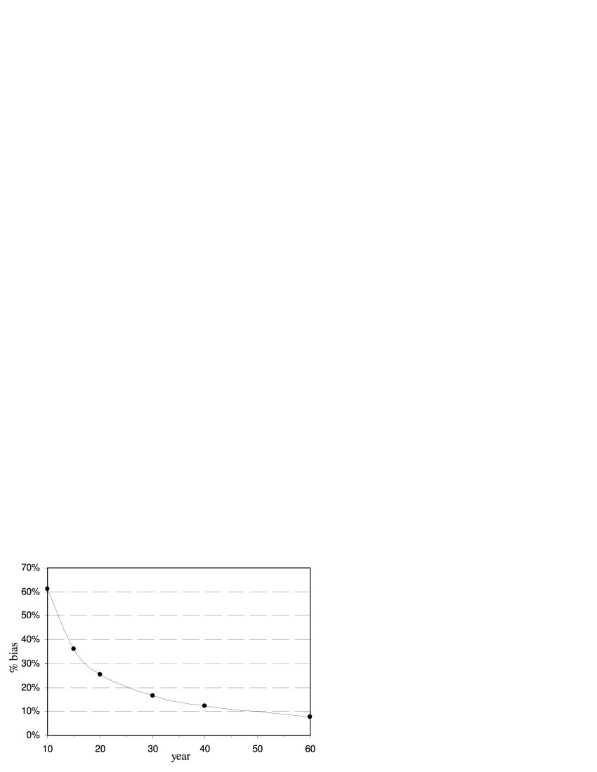
Figure 6: Relative bias (average over 100 realizations) in the 0.999 quantile of the annual loss induced by the parameter uncertainty vs the number of observation years. Losses were simulated from $Poisson(10)$ and $LN(1,2)$.

References

- [1] Basel Committee on Banking Supervision. International Convergence of Capital Measurement and Capital Standards: a revised framework. Bank for International Settlements: Basel, 2006. URL www.bis.org.
- [2] King JL. Operational Risk: Measurements and Modelling. John Wiley&Sons, 2001.
- [3] Cruz MG. Modeling, Measuring and Hedging Operational Risk. Wiley: Chichester, 2002.
- [4] Cruz MG ( (ed.)). Operational Risk Modelling and Analysis: Theory and Practice. Risk Books: London, 2004.
- [5] Panjer HH. Operational Risks: Modeling Analytics. Wiley: New York, 2006.
- [6] McNeil AJ, Frey R, Embrechts P. Quantitative Risk Management: Concepts, Techniques and Tools. Princeton University Press: Princeton, 2005.
- [7] Chernobai AS, Rachev ST, Fabozzi FJ. Operational Risk: A Guide to Basel II Capital Requirements, Models, and Analysis. John Wiley & Sons: New Jersey, 2007.
- [8] Chavez-Demoulin V, Embrechts P, Nešlehová J. Quantitative Models for Operational Risk: Extremes, Dependence and Aggregation. Journal of Banking and Finance 2006; 30(9):2635–2658.
- [9] Frachot A, Moudoulaud O, Roncalli T. Loss distribution approach in practice. The Basel Handbook: A Guide for Financial Practitioners, Ong M (ed.). Risk Books, 2004.
- [10] Aue F, Klakbrener M. Lda at work: Deutsche bank’s approach to quatifying operational risk. The Journal of Operational Risk 2006; 1(4):49–95.
- [11] Klugman SA, Panjer HH, Willmot GE. Loss Models From data to Decisions. John Wiley & Sons: New York, 1998.
- [12] Sandström A. Solvency: Models, Assessment and Regulation. Chapman & Hall/CRC: Boca Raton, 2006.
- [13] Wüthrich MV, Merz M. Stochastic Claims Reserving Methods in Insurance. John Wiley & Sons, 2008.
- [14] Moscadelli M. The modelling of operational risk: experiences with the analysis of the data collected by the Basel Committee. Bank of Italy 2004. Working paper No. 517.
- [15] Dutta K, Perry J. A tale of tails: an empirical analysis of loss distribution models for estimating operational risk capital. Federal Reserve Bank of Boston 2006. URL http://www.bos.frb.org/economic/wp/index.htm, working paper No. 06-13.
- [16] Bee M. On Maximum Likelihood Estimation of Operational Loss Distributions. Dipartimento di Economia, Universita degli Studi di Trento 2005. Discussion paper No.3.
- [17] Chernobai A, Menn C, Trück S, Rachev ST. A note on the estimation of the frequency and severity distribution of operational losses. The Mathematical Scientist 2005; 30(2).
- [18] Mignola G, Ugoccioni R. Effect of a data collection threshold in the loss distribution approach. The Journal of Operational Risk 2006; 1(4):35–47.
- [19] Luo X, Shevchenko PV, Donnelly J. Addressing impact of truncation and parameter uncertainty on operational risk estimates. The Journal of Operational Risk 2007; 2:3–26.
- [20] Baud N, Frachot A, Roncalli T. How to avoid over-estimating capital charge for operational risk? OpRisk&Compliance February 2003; URL www.opriskandcompliance.com.
- [21] Shevchenko PV, Temnov G. Modeling operational risk data reported above a time-varying threshold. The Journal of Operational Risk 2009; 4(2):19–42.
- [22] Basel Committee on Banking Supervision. Working Paper on the Regulatory Treatment of Operational Risk. Bank for International Settlements September 2001. URL www.bis.org.
- [23] Embrechts P, Klüppelberg C, Mikosch T. Modelling Extremal Events for Insurance and Finance. Springer-Verlag: Berlin, 1997. Corrected fourth printing 2003.
- [24] Nešlehová J, Embrechts P, Chavez-Demoulin V. Infinite mean models and the LDA for operational risk. Journal of Operational Risk 2006; 1(1):3–25.
- [25] Degen M, Embrechts P, Lambrigger DD. The quantitative modeling of operational risk: between g-and-h and EVT. ASTIN Bulletin 2007; 37(2):265–291.
- [26] Gustafsson J, Nielsen JP, Pritchard P, Roberts D. Operational risk guided by kernel smoothing and continuous credibility: A practioner s view. The Journal of Operational Risk 2006; 1(1):43–56.
- [27] Hess KT, Liewald A, Schmidt KD. An extension of Panjer’s recursion. ASTIN Bulletin 2002; 32(2):283–297.
- [28] Gerhold S, Schmock U, Warnung R. A generalization of Panjer’s recursion and numerically stable risk aggregation. Finance and Stochastics 2009; To appear.
- [29] Sundt B. On some extensions of Panjer’s class of counting distributions. ASTIN Bulletin 1992; 22(1):61–80.
- [30] Press WH, Teukolsky SA, Vetterling WT, Flannery BP. Numerical Recipes in C. Cambridge University Press, 2002.
- [31] Embrechts P, Frei M. Panjer recursion versus FFT for compound distributions. Mathematical Methods of Operations Research 2009; 69(3):497–508.
- [32] Schaller P, Temnov G. Efficient and precise computation of convolutions: applying FFT to heavy tailed distributions. Computational Methods in Applied Mathematics 2008; 8(2):187–200.
- [33] Luo X, Shevchenko PV. Computing tails of compound distributions using direct numerical integration. The Journal of Computational Finance 2009; To appear.
- [34] Peters GW, Johansen AM, Doucet A. Simulation of the annual loss distribution in operational risk via Panjer recursions and Volterra integral equations for Value-at-Risk and expected shortfall estimation. The Journal of Operational Risk 2007; 2(3):29–58.
- [35] Böcker K, Klüppelberg C. Operational VAR: a closed-form approximation. Risk Magazine December 2005; 12:90–93.
- [36] Böcker K, Sprittulla J. Operational VAR: meaningful means. Risk Magazine December 2006; 12:96–98.
- [37] Ergashev B. Should risk managers rely on the maximum likelihood estimation method while quantifying operational risk? The Journal of Operational Risk 2008; 3:63–86.
- [38] Lehmann EL. Theory of Point Estimation. Wiley & Sons: New York, 1983.
- [39] Efron BF, Tibshirani RJ. An Introduction to the Bootstrap. Chapman and Hall: London, 1993.
- [40] Berger JO. Statistical Decision Theory and Bayesian Analysis. 2nd edn., Springer-Verlag: New York, 1985.
- [41] Peters GW, Sisson SA. Bayesian inference, monte carlo sampling and operational risk. The Journal of Operational Risk 2006; 1(3):27–50.
- [42] Robert CP, Casella G. Monte Carlo Statistical Methods. 2nd edn., Springer Texts in Statistics: New York, 2004.
- [43] Gilks WR, Richardson S, Spiegelhalter DJ. Markov Chain Monte Carlo in practice. Chapman & Hall: London, 1996.
- [44] Peters GW, Shevchenko PV, Wüthrich MV. Model uncertainty in claims reserving within Tweedie’s compound Poisson models. ASTIN Bulletin 2009; 39(1):1–33.
- [45] Bedard M, Rosenthal JS. Optimal scaling of Metropolis algorithms: heading towards general target distributions. The Canadian Journal of Statistics 2008; 36(4):483–503.
- [46] Davis E. Theory vs reality. OpRisk&Compliance September 2006; URL www.opriskandcompliance.com/public/showPage.html?page=345305, 1 September 2006.
- [47] Shevchenko PV, Wüthrich MV. The structural modeling of operational risk via Bayesian inference: combining loss data with expert opinions. Journal of Operational Risk 2006; 1(3):3–26.
- [48] Bühlmann H, Gisler A. A Course in Credibility Theory and its Applications. Springer: Berlin, 2005.
- [49] Bühlmann H, Shevchenko PV, Wüthrich MV. A “Toy” model for operational risk quantification using credibility theory. Journal of Operational Risk 2007; 2(1):3–19.
- [50] Federal Office of Private Insurance, Bern. Swiss Solvency Test, Technical Document October 2006. URL www.bpv.admin.ch/themen/00506/00552.
- [51] Lambrigger DD, Shevchenko PV, Wüthrich MV. The quantification of operational risk using internal data, relevant external data and expert opinions. The Journal of Operational Risk 2007; 2:3–27.
- [52] Artzner P, Delbaen F, Eber JM, Heath D. Coherent measures of risk. Mathematical Finance 1999; 9:203–228.
- [53] Embrechts P, Nešlehová J, Wüthrich MV. Additivity properties for Value-at-Risk under Archimedean dependence and heavy-tailedness. Insurance: Mathematics and Economics 2009; 44:164–169.
- [54] Embrechts P, Lambrigger DD, Wüthrich MV. Multivariate extremes and the aggregation of dependent risks: examples and counter-examples. Extremes 2009; 12(2):107–127.
- [55] Frachot A, Roncalli T, Salomon E. The correlation problem in operational risk. Working paper 2004; Groupe de Recherche Opérationnelle, France.
- [56] Bee M. Copula-based multivariate models with applications to risk management and insurance. Dipartimento di Economia, Universita degli Studi di Trento 2005. URL www.gloriamundi.org, working paper.
- [57] Lindskog F, McNeil A. Common Poisson shock models: application to insurance and credit risk modelling. ASTIN Bulletin 2003; 33:209–238.
- [58] Powojowski MR, Reynolds D, Tuenter HJH. Dependent events and operational risk. ALGO Research Quarterly 2002; 5(2):65–73.
- [59] Giacometti R, Rachev ST, Chernobai A, Bertocchi M. Aggregation issues in operational risk. The Journal of Operational Risk 2008; 3(3).
- [60] Embrechts P, Puccetti G. Aggregation operational risk across matrix structured loss data. The Journal of Operational Risk 2008; 3(2):29–44.
- [61] Böcker K, Klüppelberg C. Modelling and measuring multivariate operational risk with Lévy copulas. The Journal of Operational Risk 2008; 3(2):3–27.
- [62] Böcker K, Klüppelberg C. Multivariate models for Operational Risk. Quantitative Finance 2009; To appear.
- [63] Joe H. Multivariate Models and Dependence Concepts. Chapman&Hall: London, 1997.
- [64] Nelson RB. An introduction to copulas. Springer, 1999.
- [65] Cont R, Tankov P. Financial Modelling With Jump Processes. Chapman & Hall/CRC: Boca Raton, 2004.
- [66] Marshall CL. Measuring and Managing Operational Risks in Financial Institutions. John Wiley&Sons: Singapore, 2001.
- [67] Peters GW, Shevchenko PV, Wüthrich MV. Dynamic operational risk: modeling dependence and combining different data sources of information. The Journal of Operational Risk 2009; 4(2):69–104.
- [68] Johnson NL, Kotz S, Balakrishnan N. Discrete Multivariate Distributions. JohnWiley & Sons: New York, 1997.
- [69] Shevchenko PV. Estimation of operational risk capital charge under parameter uncertainty. The Journal of Operational Risk 2008; 3(1):51–63.
- [70] Dalla Valle L. Bayesian copulae distributions, with application to operational risk management. Methodology and Computing in Applied Probability 2009; 11(1):95–115.
- [71] Mignola G, Ugoccioni R. Sources of uncertainty in modeling operational risk losses. The Journal of Operational Risk 2006; 1(2):33–50.