UMD-PP-09-034 Probing Resonant Leptogenesis at the LHC

Abstract

We explore direct collider probes of the resonant leptogenesis mechanism for the origin of matter. We work in the context of theories where the Standard Model is extended to include an additional gauged U(1) symmetry broken at the TeV scale, and where the light neutrinos obtain mass through a Type I seesaw at this scale. The $C\!P$ asymmetry that generates the observed matter-antimatter asymmetry manifests itself in a difference between the number of positive and negative like-sign dileptons $N(\ell^{+}\ell^{+})-N(\ell^{-}\ell^{-})$ that arise in the decay of the new $Z^{\prime}$ gauge boson to two right-handed neutrinos $N$, and their subsequent decay to leptons. The relatively low efficiency of resonant leptogenesis in this class of models implies that the $C\!P$ asymmetry, $\varepsilon$, is required to be sizable, i.e. of order one. In particular, from the sign of the baryon asymmetry of the Universe, an excess of antileptons is predicted. We identify the domains in $M_{Z^{\prime}}$–$M_{N}$ space where such a direct test is possible and find that with 300 fb^-1 of data and no excess found, the LHC can set the $2\sigma$ exclusion limit $\varepsilon\mathrel{\mathchoice{\vereq\displaystyle{<}}{\vereq\textstyle{<}}{\vereq\scriptstyle{<}}{\vereq\scriptscriptstyle{<}}}0.22$.

I Introduction

The origin of matter is a profound mystery. It is well known that the primordial generation of a tiny baryon-antibaryon asymmetry can explain why our present Universe consists almost exclusively of matter. The possibility that this was put in “by hand” at the beginning is not tenable since it is now generally believed that the universe underwent a period of inflation, which would have diluted this initial amount to negligible values. The observed asymmetry must therefore have been generated after the end of inflation.

In 1967, Sakharov sakharov laid down the criteria under which a baryon asymmetry can be spontaneously generated. Many particle physics scenarios have subsequently been proposed that realize Sakharov’s conditions and thereby generate the observed matter-antimatter asymmetry. In this paper, we focus on the mechanism of leptogenesis fuku , which is intimately tied to the origin of neutrino masses via the (Type I) seesaw mechanism seesaw . The basic idea is that the heavy right-handed (RH) Majorana neutrinos required for the seesaw mechanism can produce an asymmetry between leptons and antileptons using the same couplings that produce neutrino mass; this lepton asymmetry gets transformed to a baryon asymmetry with the intervention of electroweak sphaleron transitions, which are fast in the early Universe Kuzmin:1985mm .

Unfortunately, in most generic versions of the leptogenesis scenario, the RH neutrinos are superheavy and are therefore not accessible to colliders. The situation, however, is very different if there is an additional U(1) gauge symmetry broken at the TeV scale, under which the Standard Model (SM) fields are charged. In general the gauge charges of the new U(1) will forbid the $(LH)^{2}$ operator that generates Majorana neutrino mass. In such a scenario the simplest possibility for neutrino mass generation involves RH neutrinos at the TeV scale that carry charge under the additional U(1), and which are necessary for anomaly cancellation. These particles can only acquire Majorana masses once the U(1) symmetry is broken, and are therefore required to be light. The SM neutrinos have small Yukawa couplings (of order the electron Yukawa coupling) to the right-handed neutrinos, and acquire mass through a conventional Type I seesaw. In this class of theories RH neutrinos can be pair produced through decays of the $Z^{\prime}$ associated with the new gauge symmetry. Their subsequent decays $N\rightarrow\ell^{-}W^{+}$ and $N\rightarrow\ell^{+}W^{-}$ constitute a window into the dynamics underlying neutrino mass generation. In particular, the fact that the final state leptons can have the same sign constitutes concrete evidence for the Majorana nature of neutrinos. In this scenario, leptogenesis is possible provided that at least two of the RH neutrinos are quasi-degenerate. This is the so-called resonant leptogenesis mechanism resonant . Our considerations apply to this case.

Let us define the $C\!P$ asymmetry parameter relevant for the LHC,

$$\varepsilon_{i}~{}=~{}\frac{\sum_{\alpha}\left[\Gamma(N_{i}\to\ell_{\alpha}^{+}W^{-})-\Gamma(N_{i}\to\ell_{\alpha}^{-}W^{+})\right]}{\sum_{\alpha}\left[\Gamma(N_{i}\to\ell_{\alpha}^{+}W^{-})+\Gamma(N_{i}\to\ell_{\alpha}^{-}W^{+})\right]},$$ (1)

where $i=1,2,3$ and $\alpha=e,\mu,\tau$. The cosmological $C\!P$ asymmetry is usually expressed in a somewhat different way, since the RH neutrino can also decay into a $Z$ and a neutrino, or into a Higgs and a neutrino. However, in the limit $M_{N}\gg M_{W^{\pm},Z,H}$ and for the self-energy diagram which is the only one relevant for resonant leptogenesis, our definition agrees with the conventional one.

As we discuss in Section III, leptogenesis at the weak scale is very constrained in the class of models we consider, because of the $Z^{\prime}$-mediated scattering processes, $f\bar{f}\leftrightarrow NN$. The Type III seesaw case exhibits similar behavior Hambye . In fact, it is non-trivial that an allowed region in the space ($M_{Z^{\prime}}$, $M_{N}$) exists at all Frere:2008ct . The final baryon asymmetry is given by

$$\eta_{B}\simeq 10^{-2}\varepsilon\,\kappa^{\rm fin}$$ (2)

In our scenario, the efficiency factor at the end of leptogenesis, $\kappa^{\rm fin}$, is of order $10^{-7}$–$10^{-8}$ for $Z^{\prime}$ masses accessible at the LHC. It then follows that the $C\!P$ asymmetry parameter $\varepsilon$ must be of order one in order to match the observed baryon abundance, $\eta_{B}=(6.2\pm 0.15)\times 10^{-10}$ Komatsu:2008hk . This can be achieved if the RH neutrinos are degenerate to one part in $10^{14}$ resonant . An example of a simple framework in which such a spectrum of neutrinos can naturally arise is shown in Appendix B. Consequently, if the RH neutrinos satisfy the kinematic requirement that $M_{Z^{\prime}}\geq 2M_{N}$, so that the decay $Z^{\prime}\to NN$ is allowed, then $N$ must decay into leptons with order one asymmetry if leptogenesis is indeed at the origin of the observed baryon asymmetry. This “large” value of $\varepsilon$ then allows the number of positive like-sign dilepton, $N(\ell_{\alpha}^{+}\ell_{\beta}^{+})$, to be significantly different from the negative like-sign ones, $N(\ell_{\alpha}^{-}\ell_{\beta}^{-})$. This difference directly measures $(2\sum_{i}\varepsilon_{i})/(\sum_{i}1)$, as we discuss in Section IV. Therefore, an observation of this quantity constitutes a direct test of TeV-scale leptogenesis in this class of models. Specifically, as expected from leptogenesis, an excess of antileptons over leptons at the LHC is predicted by the sign of the baryon asymmetry of the universe. It should be emphasized here that the fact that large $C\!P$ asymmetries are required is entirely due to the presence of the new $Z^{\prime}$. In the standard resonant scenario at TeV scale, $C\!P$ asymmetries of order $10^{-4}$ suffice, which are much too small to be observed at colliders.

II Determining the Baryon Asymmetry

We consider the addition of an additional Abelian gauge group to the SM. For concreteness, we will take this new U(1) to be $B-L$ marshak . An alternative choice will not significantly affect our conclusions. The Lagrangian of this model differs from the SM by the usual Type I seesaw term,

$$\mathcal{L}\supset{\rm i}\overline{N_{Ri}}D_{\mu}\gamma^{\mu}N_{Ri}-h_{\alpha i}\overline{L_{L\alpha}}\tilde{\Phi}N_{Ri}-{1\over 2}M_{Ni}N_{Ri}^{T}CN_{Ri}+h.c.,$$ (3)

with $i=1,2,3$, $\alpha=e,\mu,\tau$, $L$ and $\Phi$ are $SU(2)$ doublets, $\tilde{\Phi}={\rm i}\sigma_{2}\Phi^{*}$, and $D_{\mu}=\partial_{\mu}-{\rm i}g_{1}^{\prime}Y_{B-L}B^{\prime}_{\mu}$. The charges under this group are particularly simple: $Y(Q_{L})=Y(D_{R})=Y(U_{R})=1/3$ and $Y(L_{L})=Y(E_{R})=Y(N_{R})=-1$, for quarks and leptons, respectively.

The efficiency factor $\kappa^{\rm fin}$ introduced above is determined by solving numerically the set of Boltzmann equations relevant for this model (see for instance Racker:2008hp ). In comparison to the standard Type I case, there is an additional scattering term in the equation for the evolution of the $N_{i}$ number density. In order to have enough $C\!P$ asymmetry when $M_{N}\sim 1$ TeV, the RH neutrinos need to be degenerate to a high degree resonant . However, in the computation of the efficiency factor the small mass differences do not matter, and we can assume $M_{N_{i}}\equiv M_{N}$, $i=1,2,3$. Moreover, since leptogenesis occurs in the TeV range, flavor effects Barbieri:1999ma must be included, and the three flavors are distinguished. Including flavor effects and the contributions from all RH neutrinos, we can express the final baryon asymmetry produced through leptogenesis as buch

$$\eta_{B}\simeq 10^{-2}\sum_{\alpha}N_{\Delta_{\alpha}}(z\to\infty)\simeq 10^{-2}\sum_{i,\alpha}\varepsilon_{i\alpha}\,\kappa_{i\alpha}(z\to\infty),$$ (4)

where $z=M_{N}/T$, $\Delta_{\alpha}=B/3-L_{\alpha}$ and $\sum_{\alpha}\varepsilon_{i\alpha}=\varepsilon_{i}$. The conveniently normalized number density $N_{\Delta_{\alpha}}$ or the efficiency factor $\kappa_{i\alpha}$ are found solving the relevant set of Boltzmann equations. Including only the dominant processes, i.e. decays, inverse decays, as well as scatterings mediated by $Z^{\prime}$, the latter are given by

$${{\rm d}N_{N_{i}}\over{\rm d}z}=-D(K_{i})(N_{N_{i}}-N_{N_{i}}^{\rm eq})-2\,S_{Z^{\prime}}\left(N_{N_{i}}^{2}-(N_{N_{i}}^{\rm eq})^{2}\right)\;,$$

$${{\rm d}N_{\Delta_{\alpha}}\over{\rm d}z}=\sum_{i}\varepsilon_{i\alpha}\,D(K_{i})\,(N_{N_{i}}-N_{N_{i}}^{\rm eq})-\sum_{i}W^{\rm ID}(K_{i\alpha})N_{\Delta_{\alpha}}\;,$$

where $N_{N_{i}}^{\rm eq}(z)={1\over 2}z^{2}\mathcal{K}_{2}(z)$, $D(K,z)=Kz\mathcal{K}_{1}(z)/\mathcal{K}_{2}(z)$ and $W^{\rm ID}(K,z)={1\over 4}K\mathcal{K}_{1}(z)z^{3}$, with $\mathcal{K}_{i}(z)$ being the modified Bessel function of the $i$th type. Since RH neutrinos in our model track closely equilibrium, it is possible to use the approximation ${\rm d}N_{N_{i}}/{\rm d}z\simeq{\rm d}N_{N_{i}}^{\rm eq}/{\rm d}z$ buch to write the efficiency factor $\kappa_{i\alpha}$ as

$$\kappa_{i\alpha}(z,z_{\rm in}) \simeq \int^{z}_{z_{\rm in}}{\rm d}z^{\prime}{{\rm d}N_{N_{i}}^{\rm eq}\over{\rm d}z^{\prime}}\frac{D(K_{i},z^{\prime})}{D(K_{i},z^{\prime})+4S_{Z^{\prime}}(z^{\prime})N_{N_{i}}^{\rm eq}(z^{\prime})}$$ (5)

$$\times\exp\left(-\int^{z}_{z^{\prime}}\sum_{i}W^{\rm ID}(K_{i\alpha},z^{\prime\prime}){\rm d}z^{\prime\prime}\right),$$

The flavored decay parameter is given by the ratio of the decay width to the Hubble expansion when the mass equals the temperature,

$$K_{i\alpha}={\widetilde{\Gamma}_{\rm D}(N_{i}\to L_{\alpha}\Phi+\bar{L}_{\alpha}\Phi^{\dagger})\over H(z=1)}={|h_{\alpha i}|^{2}v^{2}\over M_{N}m_{\star}},$$ (6)

with $m_{\star}=1.08\times 10^{-3}$ eV. Summing over alpha gives the total decay parameter $K_{i}=(h^{\dagger}h)_{ii}v^{2}/(M_{N}m_{\star})$. It is useful to define two typical values of the decay parameter deduced from neutrino masses: $K_{\rm sol}\equiv m_{\rm sol}/m_{\star}\simeq 8.1$ and $K_{\rm atm}\equiv m_{\rm atm}/m_{\star}\simeq 46$. Note how in general the efficiency factor in Eq. (5) depends on both $K_{i}$ and $\sum_{i}K_{i\alpha}$, and not only the sum $\sum_{i}K_{i\alpha}$ as in the usual resonant Type I case Blanchet:2006dq . The scattering rate $S_{Z^{\prime}}\equiv\gamma_{Z^{\prime}}/(Hn_{N}^{\rm eq}z)$, where $n_{N}^{\rm eq}$ is the RH neutrino equilibrium number density, and $\gamma_{Z^{\prime}}$ is a reaction density which depends on the following reduced cross section:

$$\hat{\sigma}_{Z^{\prime}}(x)={13g_{1}^{\prime 4}\over 6\pi}{\sqrt{x(x-4)^{3}}\over(x-M_{Z^{\prime}}^{2}/M_{N}^{2})^{2}+M_{Z^{\prime}}^{2}\Gamma_{Z^{\prime}}^{2}/M_{N}^{4}},$$ (7)

where $x=s/M_{N}^{2}$. The total $Z^{\prime}$ decay width in this model is given by

$$\Gamma_{Z^{\prime}}={g_{1}^{\prime 2}\over 24\pi}M_{Z^{\prime}}\left(13+3(1-4M_{N}^{2}/M_{Z^{\prime}}^{2})^{3/2}\right).$$ (8)

If one were to plot $S_{Z^{\prime}}(z)$ and $D(z)$, one would immediately see that $S_{Z^{\prime}}\gg D$ for $z\ll 1$, implying that essentially no asymmetry is produced at high temperatures $T\gg M_{N}$. The asymmetry is created once the Boltzmann suppression in $N_{N_{i}}^{\rm eq}$ starts acting, when $T\mathrel{\mathchoice{\vereq\displaystyle{<}}{\vereq\textstyle{<}}{\vereq\scriptstyle{<}}{\vereq\scriptscriptstyle{<}}}M_{N}$. It turns out that the maximal efficiency occurs at very large values of $K$, of the order of $10^{3}$–$10^{4}$ Frere:2008ct . We will be more conservative, and simply assume values of $\sum_{i}K_{i\alpha}$ that are motivated by neutrino masses, and for definiteness further assume that $K_{i\alpha}=K_{i}/3$ for each flavor $\alpha$, except in the case of normal hierarchy, where the washout in the $e$ flavor is typically suppressed Blanchet:2008zg . Note that both the assumption of flavor universality and $K\sim m_{\nu}/m_{\star}$ are conservative in the sense that relaxing them, we would get (slightly) larger efficiency factors. Since we know that $\sum_{i}K_{i}>K_{\rm sol}+K_{\rm atm}\,(2\,K_{\rm atm})$ for normal (inverted) hierarchy, and $\sum_{i}K_{i}>300$ if $m_{1}\simeq m_{2}\simeq m_{3}\simeq 0.1$ eV, i.e. for a quasi-degenerate spectrum, we will consider the following three benchmark points: $\sum_{i}K_{i\tau,\mu}=25,\sum_{i}K_{ie}=5$ for normal hierarchy, $\sum_{i}K_{i\alpha}=30$ for inverted hierarchy, and finally $\sum_{i}K_{i\alpha}=100$ for a quasi-degenerate spectrum. With reasonable assumptions about the flavored $C\!P$ asymmetries $\varepsilon_{i\alpha}$, it turns out that the normal hierarchy and inverted hierarchy cases lead to very similar results. This is because of the weak dependence of the final efficiency factor on $\sum_{i}K_{i\alpha}$. In what follows we therefore present the results for these two cases together.

We have numerically integrated Eq. (5), and assumed for concreteness that $\varepsilon_{1}=\varepsilon_{2}=\varepsilon_{3}\equiv\varepsilon$ and $K_{1}=K_{2}=K_{3}$, in order to get a typical region in the plane $M_{Z^{\prime}}$–$M_{N}$ where leptogenesis is successful. We have assumed that the production of asymmetry stops immediately once $T<T_{\rm sph}$, the sphaleron freeze-out temperature. For a Higgs mass of 120 GeV, this is given by 130 GeV Burnier . The results are shown in Figs. 1 and 2 for the value of the new gauge coupling $g^{\prime}_{1}=0.2$. The allowed regions are to the right and above the colored lines. Inside the contour of $\varepsilon=1$, the efficiency factor is $\kappa^{\rm fin}(\infty)\mathrel{\mathchoice{\vereq\displaystyle{>}}{\vereq\textstyle{>}}{\vereq\scriptstyle{>}}{\vereq\scriptscriptstyle{>}}}10^{-8}$, and inside $\varepsilon=0.1$, the efficiency factor calculated is $\kappa^{\rm fin}(\infty)\mathrel{\mathchoice{\vereq\displaystyle{>}}{\vereq\textstyle{>}}{\vereq\scriptstyle{>}}{\vereq\scriptscriptstyle{>}}}10^{-7}$. As mentioned above, we are showing only one plot for the normal and inverted hierarchy cases because the allowed regions are almost identical. We have restricted the plane to $M_{Z^{\prime}}\leq 5$ TeV and $M_{N}\leq M_{Z^{\prime}}/2$, which is favored for discovery at the LHC. Note however that leptogenesis is also successful in the region $M_{N}\geq M_{Z^{\prime}}/2$, as shown in Frere:2008ct .

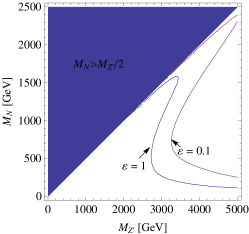
Figure 1: Regions in the space $(M_{Z^{\prime}}$–$M_{N})$ where leptogenesis can be tested for the case of normal or inverted hierarchy. The regions to the right and above the colored curves are allowed.

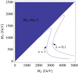
Figure 2: Same as Fig. 1 but for the case of quasi-degenerate neutrinos.

As pointed out earlier, the efficiency factor is maximal at large values of $K$. This upper bound implies an absolute lower bound for the $Z^{\prime}$ mass in order to have successful leptogenesis: $M_{Z^{\prime}}>2.6~{}(2.1)$ TeV for $g_{1}^{\prime}=0.2~{}(0.1)$. For smaller values, a $C\!P$ asymmetry parameter greater than one would be required, which is unphysical. Therefore, if a $Z^{\prime}$ with a mass below 2 TeV is discovered at the LHC, and RH neutrinos are observed with masses below $M_{Z^{\prime}}/2$, then leptogenesis is not possible, and some alternative mechanism of baryogenesis must be present. In any such scenario, the bounds on any pre-existing asymmetry derived in Blanchet:2008zg must be taken into account.

III Experimental prospects

We show in Fig. 3 the total LHC cross section calculated using CalcHEP calchep at 14 TeV to any pair of RH neutrinos, $pp\to Z^{\prime}\to NN$ rizzo . We have fixed $g_{1}^{\prime}=0.2$ and varied $M_{Z^{\prime}}$ between 2.5 and 5 TeV in steps of 500 GeV. For $M_{Z^{\prime}}=3$ TeV and $M_{N}~{}=~{}500$ GeV, we see that we obtain a total cross-section of about 1 fb, corresponding to about 300 signal events with 300 fb^-1 of data. With 1000 fb^-1 of data this increases to 1000 signal events.

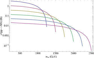
Figure 3: Total cross section $pp\to Z^{\prime}\to NN$ for $g_{1}^{\prime}=0.2$ and varying $M_{Z^{\prime}}$ between 2.5 and 5 TeV in steps of 500 GeV (top to bottom).

The decay modes of the RH neutrino that are relevant for us are $N\to\ell^{\pm}W^{\mp}$, which constitute half of the total decay rate of each RH neutrino in the limit $M_{N}\gg M_{W^{\pm},Z,H}$, as a consequence of the Goldstone boson equivalence theorem. We will concentrate on events where both right-handed neutrinos decay to charged leptons, since the backgrounds associated with such events tend to be smaller. To first order in $\varepsilon$, the asymmetry between positive and negative like-sign dileptons is given by

$${N(\ell^{+}\ell^{+})-N(\ell^{-}\ell^{-})\over N(\ell^{+}\ell^{+})+N(\ell^{-}\ell^{-})}={2\sum_{i}\varepsilon_{i}\over\sum_{i}1},$$ (9)

where we sum over all RH neutrino contributions. Therefore the difference between positive and negative like-sign dilepton events provides a direct probe of the asymmetry parameter.

We will primarily focus on events where both $W$ bosons decay hadronically. This has the advantage of avoiding ambiguities that can arise in distinguishing the leptons arising directly from RH neutrino decay from those arising subsequently from $W$ boson decay. The formula Eqn. (9) that relates the asymmetry parameter to the number of dilepton events is unaffected by this restriction. With 300 fb^-1 and no asymmetry, the expected number of such like-sign dileptons is $N(\ell^{+}\ell^{+})=N(\ell^{-}\ell^{-})=8.3\pm 2.0$ at 1$\sigma$ for $M_{Z^{\prime}}=3$ TeV and $M_{N}=500$ GeV. With 1000 fb^-1 this goes up to $27.8\pm 3.7$. If we assume $\varepsilon_{1}=\varepsilon_{2}=\varepsilon_{3}\equiv\varepsilon$, as we did for the leptogenesis analysis, and further that all such events can be identified and distinguished from background, we estimate that with 300 fb^-1 of data and no excess observed, the LHC will be able to set a 2$\sigma$ exclusion limit of order $\varepsilon<0.22$. With 1000 fb^-1 of data, this improves to $\varepsilon<0.13$. However, these assumptions clearly correspond to a best-case scenario, and a careful analysis that incorporates the effects of backgrounds, the acceptance of the detector and the challenge of signal identification in the LHC environment is required before a firm conclusion can be drawn. In this paper, we will limit ourselves to estimating the leading backgrounds, leaving a more complete study of these effects for future work.

Since the invariant mass in each event is so large, the dominant background at the LHC arises from events involving a top and anti-top that each decay leptonically, and where the charge of one of the resulting leptons is misidentified. To estimate this we calculate using CalcHEP the production cross section at the LHC for a $t\bar{t}$ pair with a total invariant mass of 3 TeV or more, and find that it is of order 10 fb. Requiring that this pair decay leptonically only reduces this to about a fb, and so additional cuts are needed. The cuts to be used depend on whether any of the leptons in the event is a tau. In events where all the leptons are electrons or muons, the requirement that the charge of one of the leptons is misidentified reduces this background to about 0.02 fb, well below the level of the signal. In addition, since these signal events involve no missing energy, this can be used to reduce the background. Finally, requiring that the invariant mass of each $\ell W$ pair add up to the mass of the $N$ provides another very strong constraint. We conclude that this background is under control.

Background events involving one or more taus are more difficult to constrain, since tau charge identification is in general less reliable unless the tau decays leptonically. In addition, since tau events always involve missing energy, such a cut cannot be used. In events where at least one of the leptons is an electron or a muon (about $90\%$ of events) requiring that the invariant mass of this $\ell W$ pair add up to the mass of the $N$ can be used to reduce the background. Furthermore, the fact that the direction of the invisible decay products of a highly boosted tau will align almost exactly with that of the visible decay products leads to a constraint on the direction of the missing energy in the event, and also to a separate invariant mass constraint. The same fact can be used to restrict the background even in events where both the leptons are taus. Separately, the fact that the mass of the RH neutrino is in general much larger than the mass of the top quark means that the angular distributions of their decay products are very different, leading to additional constraints.

Another possible background at the LHC arises from $jjW^{+}W^{+}$, with the $W$’s decaying leptonically. We have studied this background using MadGraph/MadEvent madgraph . Requiring that the energy of the visible particles in the event be greater than 3 TeV, that the transverse momentum of each lepton be at least 100 GeV, and that the total missing energy in the event be less than 50 GeV reduces this background to below 0.005 fb. We have verified that these cuts do not significantly affect the signal. An identical set of cuts can be used to kill the background arising from $jjW^{+}W^{-}$, with the charge of one of the leptons misidentified. This analysis suggests that the backgrounds are under control, though further study is required before a firm conclusion can be drawn.

While we have focused on events where both $W$ bosons decay into hadrons, events where one $W$ boson decays leptonically can also be used to extract information about the $C\!P$ asymmetry parameter $\varepsilon$, provided all the leptons in the event are electrons or muons. All the missing energy in such events is associated with a single neutrino, allowing the corresponding $W$ boson to be reconstructed. The lepton arising from decay of the $W$ can then be identified and distinguished from the leptons arising directly from RH neutrino decay. The primary background to such events arises from $jjWZ$, and can be made negligible after cuts.

It is also possible to calculate $\varepsilon$ from events where only one of the RH neutrinos decays to a charged lepton and $W$, while the other decays to a neutrino and $Z$, or alternatively to a neutrino and Higgs. Although the SM backgrounds are potentially larger, there are more such events than like-sign dilepton events. $\varepsilon$ is related to the asymmetry in the number of events with positively charged leptons relative to negatively charged leptons.

$${N(\ell^{+})-N(\ell^{-})\over N(\ell^{+})+N(\ell^{-})}={\sum_{i}\varepsilon_{i}\over\sum_{i}1},$$ (10)

Therefore, this class of events can be used as an independent measure of the value of $\varepsilon$.

In order to achieve order one values for the $C\!P$ asymmetry, we must be close to the resonance region $M_{j}-M_{i}\sim\Gamma/2$, where interference effects may be important. However, for perturbation theory in the computation of the $C\!P$ asymmetry to be applicable, we require $M_{j}-M_{i}\mathrel{\mathchoice{\vereq\displaystyle{>}}{\vereq\textstyle{>}}{\vereq\scriptstyle{>}}{\vereq\scriptscriptstyle{>}}}3\,\Gamma/2$  Anisimov:2005hr , which corresponds to $\varepsilon\mathrel{\mathchoice{\vereq\displaystyle{<}}{\vereq\textstyle{<}}{\vereq\scriptstyle{<}}{\vereq\scriptscriptstyle{<}}}0.3$. In Appendix A, we explicitly verify that interference effects arise only at order $\varepsilon^{3}$ for the $C\!P$ violating observable in Eq. (9), and at order $\varepsilon^{2}$ in the rates. Then, for $\varepsilon\mathrel{\mathchoice{\vereq\displaystyle{<}}{\vereq\textstyle{<}}{\vereq\scriptstyle{<}}{\vereq\scriptscriptstyle{<}}}0.3$, the corrections to our results from interference are not more than 10%.

An important element for resonant leptogenesis is the presence of at least two degenerate RH neutrinos. The extreme degeneracy in their masses implies that it will not be possible to determine the number of RH neutrinos based on invariant mass measurements. Nevertheless, by measuring their branching ratios into leptons of various flavors, it may be possible to distinguish the cases of one, two and three RH neutrinos, even in the absence of any observed $C\!P$ asymmetry. The decay probability of one RH neutrino into a certain lepton flavor (either lepton or antilepton) is given by

$$P_{i\alpha}={|h_{\alpha i}|^{2}\over(h^{\dagger}h)_{ii}}.$$ (11)

Clearly the sum of the probabilities must equal one: $\sum_{\alpha}P_{i\alpha}=1$, for $i=1,2$ and 3. Then, the probability of a given dilepton event to involve the flavors $\alpha$ and $\beta$, which can be directly measured at the LHC, is

$$P(\ell_{\alpha}\ell_{\beta})={\sum_{i}P_{i\alpha}P_{i\beta}\over\sum_{i}1},$$ (12)

where $\alpha,\beta=e,\mu,\tau$, and $i$ runs over the RH neutrinos (1, 2 or 3). Note that the tree level expressions used here are enough for our purposes since the total rates into leptons plus antileptons are only corrected by $\epsilon^{2}$ as described above, contrary to the difference in rates into leptons versus antileptons, which goes like $\varepsilon$. We have the additional constraint that $\sum_{\alpha,\beta}P(\ell_{\alpha}\ell_{\beta})=1$, which implies that one of the six equations in Eq. (12) is redundant. With only one RH neutrino, say $N_{1}$, we have five equations for two unknowns, $P_{1e}$ and $P_{1\mu}$ ($P_{1\tau}$ is known from the sum of probabilities), which means that the system is highly overconstrained. If no consistent solution to these five equations can be found, it means that there must be more than one RH neutrino. If there are two RH neutrinos, say $N_{1}$ and $N_{2}$, we have five equations for the four unknowns $P_{1e}$, $P_{1\mu}$, $P_{2e}$ and $P_{2\mu}$ and so the system is still overconstrained. Therefore this case can potentially also be distinguished from that of three RH neutrinos.

IV Conclusion

We have shown that in a model with TeV-scale RH neutrinos and $Z^{\prime}$ gauge boson, resonant leptogenesis is possible, and requires a large (order one) $C\!P$ asymmetry to work. The allowed range for leptogenesis in the space $M_{Z^{\prime}}$–$M_{N}$ is very constrained in the LHC-favored situation $M_{N}<M_{Z^{\prime}}/2$, and favors larger values of the $Z^{\prime}$ mass, $M_{Z^{\prime}}>2$ TeV. The large $C\!P$ asymmetry required in the decay of the RH neutrinos may have observable consequences at the LHC, in particular an asymmetry in the number of positive and negative like-sign dilepton events. Specifically, the sign of the baryon asymmetry of the Universe implies an excess of anti-leptons over leptons. If no excess is observed, we find that with 300 fb^-1 of integrated luminosity the LHC will be able to exclude at 2$\sigma$ that $\varepsilon\mathrel{\mathchoice{\vereq\displaystyle{>}}{\vereq\textstyle{>}}{\vereq\scriptstyle{>}}{\vereq\scriptscriptstyle{>}}}0.22$. Finally, although the RH neutrino masses are essentially identical, their couplings to leptons are not, and we show that some simple linear algebra considerations allow us to distinguish the cases of one, two and three degenerate RH neutrinos even in the absence of any observed $C\!P$ asymmetry.

Appendix A Interference effects

In the following we want to compute the parameter dependence of the interference terms in the process $Z^{\prime}\to\ell_{\alpha}\Phi\ell_{\beta}\Phi$, where RH neutrinos are exchanged in the intermediate step.

A.1 Field theory derivation

The amplitude for the process $Z^{\prime}(p_{Z^{\prime}})\to\ell_{\alpha}(k_{1})\Phi(k_{2})\ell_{\beta}(k_{1}^{\prime})\Phi(k_{2}^{\prime})$ is given by

$$\mathcal{M}(\ell_{\alpha}\ell_{\beta}) = g_{1}^{\prime}\bar{u}_{\alpha}(k_{1})P_{R}[h_{\alpha 1}S_{11}(p)+h_{\alpha 2}S_{12}(p)]\gamma_{\mu}\gamma_{5}$$ (13)

$$\varepsilon^{\mu}(p_{Z^{\prime}})[h_{\beta 1}S_{11}(p^{\prime})+h_{\beta 2}S_{12}(p^{\prime})]P_{R}v_{\beta}(k_{1}^{\prime})$$

$$+ g_{1}^{\prime}\bar{u}_{\alpha}(k_{1})P_{R}[h_{\alpha 1}S_{21}(p)+h_{\alpha 2}S_{22}(p)]\gamma_{\mu}\gamma_{5}$$

$$\varepsilon^{\mu}(p_{Z^{\prime}})[h_{\beta 1}S_{21}(p^{\prime})+h_{\beta 2}S_{22}(p^{\prime})]P_{R}v_{\beta}(k_{1}^{\prime}).$$

Following Anisimov:2005hr we decompose the propagator into chiral components

$$S_{ij}(p) = P_{R}S_{ij}^{RR}(p^{2})+P_{L}S_{ij}^{LL}(p^{2})$$ (14)

$$+ P_{L}\displaystyle{\not}pS_{ij}^{LR}(p^{2})+P_{R}\displaystyle{\not}pS_{ij}^{RL}(p^{2}).$$

It can then be easily shown that the only non-zero components are given by

$$S^{RR}(p^{2})[\ldots]p\!\!/^{\prime}S^{LR}(p^{\prime 2})+\displaystyle{\not}pS^{RL}(p^{2})[\ldots]S^{RR}(p^{\prime 2}).$$ (15)

The renormalized and resummed matrices of propagators $S^{RR}$, $S^{LL}$, $S^{LR}$ and $S^{RL}$ can be found in Anisimov:2005hr and will not be reproduced here. The crucial parameters for the following discussion are the poles of the propagators, given to leading order in the small Yukawa couplings by Anisimov:2005hr

$$s_{i}\simeq M_{i}^{2}-iM_{i}\Gamma_{i}\,.$$ (16)

We have to evaluate now the modulus squared of the amplitude (13). We will omit for clarity the spinor and gamma matrices product since they will be common to all terms. We obtain

$$|\mathcal{M}|^{2}/g_{1}^{\prime 2} =$$ (17)

$$|h_{\alpha 1}h_{\beta 1}S_{11}(p)S_{11}(p^{\prime})+h_{\alpha 1}h_{\beta 2}S_{11}(p)S_{12}(p^{\prime})$$

$$+h_{\alpha 2}h_{\beta 1}S_{12}(p)S_{11}(p^{\prime})+h_{\alpha 2}h_{\beta 2}S_{12}(p)S_{12}(p^{\prime})|^{2}$$

$$+|h_{\alpha 1}h_{\beta 1}S_{21}(p)S_{21}(p^{\prime})+h_{\alpha 1}h_{\beta 2}S_{21}(p)S_{22}(p^{\prime})$$

$$+h_{\alpha 2}h_{\beta 1}S_{22}(p)S_{21}(p^{\prime})+h_{\alpha 2}h_{\beta 2}S_{22}(p)S_{22}(p^{\prime})|^{2}$$

$$+2{\rm Re}\left[\left(h_{\alpha 1}h_{\beta 1}S_{11}(p)S_{11}(p^{\prime})+h_{\alpha 1}h_{\beta 2}S_{11}(p)S_{12}(p^{\prime})\right.\right.$$

$$\left.\left.+h_{\alpha 2}h_{\beta 1}S_{12}(p)S_{11}(p^{\prime})+h_{\alpha 2}h_{\beta 2}S_{12}(p)S_{12}(p^{\prime})\right)^{\star}\right.$$

$$\left.\times\left(h_{\alpha 1}h_{\beta 1}S_{21}(p)S_{21}(p^{\prime})+h_{\alpha 1}h_{\beta 2}S_{21}(p)S_{22}(p^{\prime})\right.\right.$$

$$\left.\left.+h_{\alpha 2}h_{\beta 1}S_{22}(p)S_{21}(p^{\prime})+h_{\alpha 2}h_{\beta 2}S_{22}(p)S_{22}(p^{\prime})\right)\right].$$

Note that we omit the upper scripts $RR$, $RL$ or $LR$ because the distinction will become irrelevant on mass shell. Keeping only first order terms in the off-diagonal elements of the propagator matrix $S_{12}=S_{21}$ and we obtain

$$|\mathcal{M}|^{2}/g_{1}^{\prime 2} = |h_{\alpha 1}|^{2}|h_{\beta 1}|^{2}|S_{11}(p)|^{2}|S_{11}(p^{\prime})|^{2}$$ (18)

$$+ |h_{\alpha 2}|^{2}|h_{\beta 2}|^{2}|S_{22}(p)|^{2}|S_{22}(p^{\prime})|^{2}$$

$$+ 2{\rm Re}\left(h_{\alpha 1}^{\star}h_{\beta 1}^{\star}h_{\alpha 2}h_{\beta 2}S_{11}^{\star}(p)S_{22}(p)S_{11}^{\star}(p^{\prime})S^{\star}_{22}(p^{\prime})\right)$$

$$+ 2|h_{\alpha 1}|^{2}|S_{11}(p)|^{2}{\rm Re}\left(h_{\beta 1}^{\star}h_{\beta 2}S_{11}^{\star}(p^{\prime})S_{12}(p^{\prime})\right)$$

$$+ 2|h_{\alpha 2}|^{2}|S_{22}(p)|^{2}{\rm Re}\left(h_{\beta 1}^{\star}h_{\beta 2}S_{21}^{\star}(p^{\prime})S_{22}(p^{\prime})\right)$$

$$+ 2|h_{\beta 1}|^{2}|S_{11}(p^{\prime})|^{2}{\rm Re}\left(h_{\alpha 1}^{\star}h_{\alpha 2}S_{11}^{\star}(p)S_{12}(p)\right)$$

$$+ 2|h_{\beta 2}|^{2}|S_{22}(p^{\prime})|^{2}{\rm Re}\left(h_{\alpha 1}^{\star}h_{\alpha 2}S_{21}^{\star}(p)S_{22}(p)\right)$$

$$+ 2|h_{\alpha 1}|^{2}{\rm Re}\left(h_{\beta 1}^{\star}h_{\beta 2}S_{11}^{\star}(p)S_{21}(p)S_{11}^{\star}(p^{\prime})S_{22}(p^{\prime})\right)$$

$$+ 2|h_{\alpha 2}|^{2}{\rm Re}\left(h_{\beta 1}^{\star}h_{\beta 2}S_{12}^{\star}(p)S_{22}(p)S_{11}^{\star}(p^{\prime})S_{22}(p^{\prime})\right)$$

$$+ 2|h_{\beta 1}|^{2}{\rm Re}\left(h_{\alpha 1}^{\star}h_{\alpha 2}S_{11}^{\star}(p)S_{22}(p)S_{11}^{\star}(p^{\prime})S_{21}(p^{\prime})\right)$$

$$+ 2|h_{\beta 2}|^{2}{\rm Re}\left(h_{\alpha 1}^{\star}h_{\alpha 2}S_{11}^{\star}(p)S_{22}(p)S_{12}^{\star}(p^{\prime})S_{22}(p^{\prime})\right).\hskip 14.22636pt$$

The first two terms are the ones that are naively expected if the RH neutrino propagation is incoherent. In the on-shell limit, within a narrow width approximation, they yield, respectively,

$$|S_{ii}(p)|^{2} \propto {1\over p^{2}-s_{i}}{1\over p^{2}-s_{i}^{\star}}$$ (19)

$$\longrightarrow {\pi\over\Gamma_{i}M_{i}}\,\delta(p^{2}-M_{i}^{2})\,.$$

They correspond to two incoherent RH neutrinos produced in $Z^{\prime}$ decay which subsequently decay into a lepton-Higgs pair. The third term in Eq. (18) is new. It is an interference term that does not rely on the mixing, or alternatively on the off-diagonal elements of the matrix of propagators. Let us analyze this term in detail:

$$S_{11}^{\star}(p)S_{22}(p) \propto {1\over p^{2}-s_{1}^{\star}}{1\over p^{2}-s_{2}}$$ (20)

$$\longrightarrow{2\pi i\over s_{2}-s_{1}^{\star}}\delta(p^{2}-\overline{M}^{2})$$

$$={2\pi i(M_{2}^{2}-M_{1}^{2}+i(\Gamma_{1}M_{1}+\Gamma_{2}M_{2}))\over(M_{2}^{2}-M_{1}^{2})^{2}+(\Gamma_{1}M_{1}+\Gamma_{2}M_{2})^{2}}\delta(p^{2}-\overline{M}^{2})\,,\hskip 14.22636pt$$

where $\overline{M}^{2}\equiv(M_{1}^{2}+M_{2}^{2})/2$. A similar term arises from $S_{11}^{\star}(p^{\prime})S_{22}(p^{\prime})$. Dropping the delta functions and the $\pi$ factors, we are left with the evaluation of

$${\rm Re}\left\{{-\left[M_{2}^{2}-M_{1}^{2}+i(\Gamma_{1}M_{1}+\Gamma_{2}M_{2})\right]^{2}\over\left[(M_{2}^{2}-M_{1}^{2})^{2}+(\Gamma_{1}M_{1}+\Gamma_{2}M_{2})^{2}\right]^{2}}h_{\alpha 1}^{\star}h_{\beta 1}^{\star}h_{\alpha 2}h_{\beta 2}\right\}$$

$$={-(M_{2}^{2}-M_{1}^{2})^{2}+(\Gamma_{1}M_{1}+\Gamma_{2}M_{2})^{2}\over\left[(M_{2}^{2}-M_{1}^{2})^{2}+(\Gamma_{1}M_{1}+\Gamma_{2}M_{2})^{2}\right]^{2}}{\rm Re}(h_{\alpha 1}^{\star}h_{\beta 1}^{\star}h_{\alpha 2}h_{\beta 2})+$$

$${2(M_{2}^{2}-M_{1}^{2})(\Gamma_{1}M_{1}+\Gamma_{2}M_{2})\over\left[(M_{2}^{2}-M_{1}^{2})^{2}+(\Gamma_{1}M_{1}+\Gamma_{2}M_{2})^{2}\right]^{2}}{\rm Im}(h_{\alpha 1}^{\star}h_{\beta 1}^{\star}h_{\alpha 2}h_{\beta 2}).$$ (21)

For the rate into two antileptons, $|\mathcal{M}(\bar{\ell}_{\alpha}\bar{\ell}_{\beta})|^{2}$, only the replacement $h_{\alpha i}\to h_{\alpha i}^{\star}$ needs to be made in Eq. (21). The difference in the rates into two leptons and two antileptons is then given by

$$|\mathcal{M}(\ell_{\alpha}\ell_{\beta})|^{2}-|\mathcal{M}(\bar{\ell}_{\alpha}\bar{\ell}_{\beta})|^{2}\propto\epsilon_{+}^{2}\,{\Gamma_{1}M_{1}+\Gamma_{2}M_{2}\over M_{2}^{2}-M_{1}^{2}}\,,$$ (22)

where we introduced the parameter

$$\epsilon_{\pm}\equiv{(M_{2}^{2}-M_{1}^{2})M_{2}\Gamma_{2}\over(M_{2}^{2}-M_{1}^{2})^{2}+(\Gamma_{1}M_{1}\pm\Gamma_{2}M_{2})^{2}}.$$ (23)

Note that in the following we shall assume a hierarchy between $M_{1}\Gamma_{1}$ and $M_{2}\Gamma_{2}$ such that $\epsilon_{+}\simeq\epsilon_{-}=\epsilon$. In the limit $M_{2}-M_{1}\gg\Gamma/2$, the overall suppression of the third term in Eq. (18) is therefore $\epsilon^{3}$. As for the sum of the rates $|\mathcal{M}(\ell_{\alpha}\ell_{\beta})|^{2}+|\mathcal{M}(\bar{\ell}_{\alpha}\bar{\ell}_{\beta})|^{2}$ it can be readily seen that it is suppressed as $\epsilon^{2}$.

For future use, we note that the $C\!P$ asymmetry in resonant leptogenesis, summed over flavor, is given by Anisimov:2005hr

$$\varepsilon_{1}={{\rm Im}(h^{\dagger}h)_{12}^{2}\over(h^{\dagger}h)_{11}(h^{\dagger}h)_{22}}\,\epsilon_{-}\,.$$ (24)

Terms 4 to 7 in Eq. (18) involve mixing. The prefactors $|S_{ii}(p)|^{2}$ yield delta functions as in Eq. (19). The more interesting part is the real part. We have

$$S_{11}^{\star}(p^{\prime})S_{12}(p^{\prime}) = {1\over p^{\prime 2}-s_{1}^{\star}}\times$$ (25)

$${M_{1}M_{2}\Sigma_{12}^{R}+p^{\prime 2}\Sigma_{21}^{R}+M_{1}\Sigma_{12}^{M\star}+M_{2}\Sigma_{12}^{M}\over(p^{\prime 2}-s_{1})(p^{\prime 2}-s_{2})}$$

$$= {\pi\delta(p^{\prime 2}-M_{1}^{2})\over\Gamma_{1}M_{1}}\,X_{12}\,,$$

where $\Sigma^{R}$ and $\Sigma^{M}$ are defined in Anisimov:2005hr [Eqs. (9)–(12)], and with

$$X_{12}\equiv{M_{1}M_{2}\Sigma_{12}^{R}+M_{1}^{2}\Sigma_{21}^{R}+M_{1}\Sigma_{12}^{M\star}+M_{2}\Sigma_{12}^{M}\over(s_{1}-s_{2})}.$$ (26)

To evaluate ${\rm Re}\left(h_{\beta 1}^{\star}h_{\beta 2}X_{12}\right)$, we multiply first the numerator and the denominator by $(s_{1}-s_{2})^{\star}$, noting that

$$|s_{1}-s_{2}|^{2}=(M_{1}^{2}-M_{2}^{2})^{2}+(\Gamma_{1}M_{1}-\Gamma_{2}M_{2})^{2}.$$ (27)

Then we turn to the rate into antileptons and find it to be proportional to ${\rm Re}\left(h_{\beta 1}h_{\beta 2}^{\star}X_{21}\right)$, where $X_{21}$ is equal to $X_{12}$ modulo the transformation of the Yukawas $h\to h^{\star}$. The difference $|\mathcal{M}(\ell_{\alpha}\ell_{\beta})|^{2}-|\mathcal{M}(\bar{\ell}_{\alpha}\bar{\ell}_{\beta})|^{2}$, summed over $\beta$ for convenience, is then found to be precisely proportional to $\varepsilon_{1}$ as defined in Eq. (24).

The fifth term in Eq. (18) will give another $\varepsilon_{1}$ contribution (from the other leg), whereas the terms 6 and 7 in Eq. (18) are the $\varepsilon_{2}$ contributions.

Now let us turn to terms 8 to 11 in Eq. (18). We will only show explicitly how to work out term 8, but the other terms follow in a similar fashion. From Eqs. (20) and (25) we have that

$${\rm Re}\left[h_{\beta 1}^{\star}h_{\beta 2}S^{\star}_{11}(p)S_{21}(p)S^{\star}_{11}(p^{\prime})S_{22}(p^{\prime})\right]=$$

$${\rm Re}\left[h_{\beta 1}^{\star}h_{\beta 2}S^{\star}_{11}(p)S_{21}(p)\right]{\rm Re}\left[S^{\star}_{11}(p^{\prime})S_{22}(p^{\prime})\right]$$

$$-{\rm Im}\left[h_{\beta 1}^{\star}h_{\beta 2}S^{\star}_{11}(p)S_{21}(p)\right]{\rm Im}\left[S^{\star}_{11}(p^{\prime})S_{22}(p^{\prime})\right]$$

$$\propto{2\pi^{2}\over M_{1}\Gamma_{1}}\delta(p^{2}-M_{1}^{2})\delta(p^{\prime 2}-M_{2}^{2})\times$$

$$\left[{\rm Re}\left(h_{\beta 1}^{\star}h_{\beta 2}X_{12}\right){M_{1}\Gamma_{1}+M_{2}\Gamma_{2}\over|s_{2}-s_{1}^{\star}|^{2}}\right.$$

$$\left.\hskip 28.45274pt-{\rm Im}\left(h_{\beta 1}^{\star}h_{\beta 2}X_{12}\right){M_{2}^{2}-M_{1}^{2}\over|s_{2}-s_{1}^{\star}|^{2}}\right]$$ (28)

When estimating the difference of rates into leptons and antileptons, we have already seen that ${\rm Re}\left(h_{\beta 1}^{\star}h_{\beta 2}X_{12}\right)$ gives rise to a term proportional to the $C\!P$ asymmetry $\varepsilon_{1}$. But here it is multiplied by another small term in the limit $M_{2}-M_{1}\gg\Gamma/2$, so that the overall suppression is equivalent to Eq. (22), namely an $\epsilon^{3}$ suppression.

As for the second term in the square bracket, there is an obvious suppression by $\epsilon$ to start with. The difference of rates into leptons and antileptons yields another suppression. It is given by

$${\rm Im}\left(h_{\beta 1}^{\star}h_{\beta 2}X_{12}\right) - {\rm Im}\left(h_{\beta 2}^{\star}h_{\beta 1}X_{21}\right)=$$ (29)

$${\rm Im}\left(h_{\beta 1}^{\star}h_{\beta 2}\right)\left({\rm Re}X_{12}+{\rm Re}X_{21}\right)$$

$$+{\rm Re}\left(h_{\beta 1}^{\star}h_{\beta 2}\right)\left({\rm Im}X_{12}-{\rm Im}X_{21}\right).$$

The first term on the right-hand side is given to leading order by

$${\rm Re}X_{12}+{\rm Re}X_{21} \simeq \left({\rm Im}\Sigma_{12}+{\rm Im}\Sigma_{21}\right){M_{2}\Gamma_{2}-M_{1}\Gamma_{1}\over|s_{2}-s_{1}|^{2}}$$ (30)

$$={M_{1}(M_{1}+M_{2})\over 8\pi}{\rm Re}(h^{\dagger}h)_{21}{M_{2}\Gamma_{2}-M_{1}\Gamma_{1}\over|s_{2}-s_{1}|^{2}},$$

which implies an additional suppression by $\epsilon^{2}$, such that the overall suppression is $\epsilon^{3}$. As before, the sum of rates into leptons and antileptons is only suppressed by a factor $\epsilon^{2}$.

The second term yields

$${\rm Im}X_{12}-{\rm Im}X_{21} \simeq \left({\rm Re}\Sigma_{12}-{\rm Re}\Sigma_{21}\right){\Gamma_{2}M_{2}-\Gamma_{1}M_{1}\over|s_{2}-s_{1}|^{2}}$$ (31)

$$={M_{1}(M_{2}-M_{1})\over 8\pi}{\rm Im}(h^{\dagger}h)_{12}{\Gamma_{2}M_{2}-\Gamma_{1}M_{1}\over|s_{2}-s_{1}|^{2}},$$

which is even more suppressed than the previous term.

We have therefore shown that the $C\!P$-violating interference effects are at least suppressed by three powers of $\epsilon$, while the $C\!P$ conserving ones are suppressed by two powers only.

A.2 Oscillation derivation

We employ here the formalism which was successfully used to describe $K^{0}$–$\overline{K}^{0}$ and $B^{0}$–$\overline{B}^{0}$ oscillations. The first part of our discussion will follow closely Covi:1996fm , where leptogenesis from mixed particle decays was considered.

In the non-relativistic limit the squared Hamiltonian can be decomposed as

$$\hat{H}_{ij}=M_{ij}-{\rm i}\,\Gamma_{ij}/2$$ (32)

where the renormalized mass matrix $M$ includes the dispersive parts of the self-energy diagram while the matrix $\Gamma$ arises from the absorptive part alone. The squared Hamiltonian can be diagonalized by a non-unitary matrix $V$,

$$(V\,\hat{H}\,V^{-1})_{ij}=\sqrt{s_{i}}\delta_{ij}\,,$$ (33)

and the squared eigenvalues of the Hamiltonian coincide with the poles of the propagator defined in Eq. (16).

An important ingredient in the present formalism is the proper identification of the initial state. In our case, the $Z^{\prime}$ is produced in the $s$ channel, and then decays into a pair of RH neutrinos. The only gauge invariant combination is $|N^{\prime}_{1}\overline{N}^{\prime}_{1}+N^{\prime}_{2}\overline{N}^{\prime}_{2}\rangle$, where $N^{\prime}_{i}$ are propagation eigenstates. The decay rate into dileptons will then be proportional to

$$|\mathcal{M}(\ell_{\alpha}\ell_{\beta})|^{2}=|\langle\ell_{\alpha}\Phi\ell_{\beta}\Phi|H_{\rm int}^{2}|N^{\prime}_{1}\overline{N}^{\prime}_{1}+N^{\prime}_{2}\overline{N}^{\prime}_{2}\rangle|^{2}\,.$$ (34)

Expanding this expression we obtain

$$|\mathcal{M}(\ell_{\alpha}\ell_{\beta})|^{2} = |\langle\ell_{\alpha}\Phi|H_{\rm int}|N^{\prime}_{1}\rangle|^{2}|\langle\ell_{\beta}\Phi|H_{\rm int}|N^{\prime}_{1}\rangle|^{2}$$ (35)

$$+ |\langle\ell_{\alpha}\Phi|H_{\rm int}|N^{\prime}_{2}\rangle|^{2}|\langle\ell_{\beta}\Phi|H_{\rm int}|N^{\prime}_{2}\rangle|^{2}$$

$$+ 2\,{\rm Re}\left(\langle\ell_{\alpha}\Phi|H_{\rm int}|N^{\prime}_{2}\rangle\langle\ell_{\beta}\Phi|H_{\rm int}|N^{\prime}_{2}\rangle\right.$$

$$\left.\langle N^{\prime}_{1}|H_{\rm int}^{\dagger}|\ell_{\alpha}\Phi\rangle\langle N^{\prime}_{1}|H_{\rm int}^{\dagger}|\ell_{\beta}\Phi\rangle\right)\,.$$

Evolving the propagation eigenstates in the usual way, we have that

$$T_{i\beta}(t) \equiv \langle\ell_{\beta}\Phi|H_{\rm int}|N^{\prime}_{i}(t)\rangle$$ (36)

$$= (h_{\beta 1}V_{1i}^{-1}+h_{\beta 2}V_{2i}^{-1})\,e^{-{\rm i}\,\sqrt{s_{i}}t}.$$

Let us now compute the first term in Eq. (35) allowing for oscillation, namely $|T_{1\alpha}(t)|^{2}$ to first order in the off-diagonal elements of the mixing matrix $V$. Note that $V_{11}=V_{22}=1+\mathcal{O}(h^{2}/(16\pi^{2}))$. We obtain

$$|T_{1\beta}(t)|^{2} = |h_{\beta 1}|^{2}e^{{\rm i}(\sqrt{s_{1}}^{\star}-\sqrt{s_{1}})t}$$ (37)

$$+ 2\,{\rm Re}\left(h_{\beta 1}^{\star}h_{\beta 2}V_{21}^{-1}e^{{\rm i}(\sqrt{s_{1}}^{\star}-\sqrt{s_{1}})t}\right)\,.$$

Carrying out the time integration from 0 to infinity, we have

$$\int_{0}^{\infty}dt\,|T_{1\beta}(t)|^{2} = |h_{\beta 1}|^{2}{1\over\Gamma_{1}}$$ (38)

$$+ 2{1\over\Gamma_{1}}{\rm Re}\left(h_{\beta 1}^{\star}h_{\beta 2}V_{21}^{-1}\right)$$

and $V_{21}^{-1}=-V_{21}$ coincides with $X_{12}$ defined in Eq. (26).

We obtain the first term in Eq. (35) by multiplying with the same expression as derived in Eq. (38) except for the replacement $\beta\to\alpha$. To first order in $V_{21}$, we obtain five terms, which correspond to the first, fourth, sixth term in Eq. (18). Note that the factor $g_{1}^{\prime 2}\pi/M$ difference between this formalism and the previous one can be trivially explained when computing explicitly the total cross-section $q\bar{q}\to\ell_{\alpha}\ell_{\beta}\Phi\Phi$.

It is easy to obtain the corresponding expressions for $|T_{2\beta}(t)|^{2}$, and the second term in Eq. (35) readily yields terms 2, 5, 7 in Eq. (18).

For the third term in Eq. (35) we have that

$$T_{1\beta}^{\star}(t)T_{2\beta}(t) = h_{\beta 1}^{\star}h_{\beta 2}e^{{\rm i}(\sqrt{s_{1}}^{\star}-\sqrt{s_{2}})t}$$ (39)

$$+ |h_{\beta 1}|^{2}\,V_{12}^{-1}e^{{\rm i}(\sqrt{s_{1}}^{\star}-\sqrt{s_{1}})t}$$

$$+ |h_{\beta 2}|^{2}\,(V_{21}^{-1})^{\star}e^{{\rm i}(\sqrt{s_{2}}^{\star}-\sqrt{s_{2}})t}$$

to first order in $V_{21}$, and the time integration yields

$$\int_{0}^{\infty}dt\,T_{1\beta}^{\star}(t)T_{2\beta}(t) = h_{\beta 1}^{\star}h_{\beta 2}{{\rm i}\,2M_{1}\over s_{2}-s_{1}^{\star}}$$ (40)

$$+ {1\over\Gamma_{1}}|h_{\beta 1}|^{2}\,V_{12}^{-1}$$

$$+ {1\over\Gamma_{2}}|h_{\beta 2}|^{2}\,(V_{21}^{-1})^{\star}\,.$$

A similar result can be obtained for $T_{1\alpha}^{\star}(t)T_{2\alpha}(t)$. Multiplying the two expressions, we obtain the third term in Eq. (18), as well as terms 8 to 11. This completes the proof of the equivalence between the field theory formalism and the oscillation one.

Appendix B A Framework for Natural Resonant Leptogenesis

In this section, we outline a framework which naturally realizes resonant leptogenesis at the TeV scale. In particular, the following features that are necessary for the scenario we have proposed to be viable will be shown to emerge naturally in this scheme.

• A simple understanding of why the RH neutrino masses naturally lie close to the weak scale.

• A straightforward explanation for the smallness of neutrino masses, and for the quasi-degeneracy of the RH neutrinos.

• A natural understanding of why the asymmetry in RH neutrino decays tends to be of order one.

We begin by extending the electroweak gauge group of the SM from $SU(2)_{L}\times U(1)_{Y}$ to $SU(2)_{L}\times U(1)_{Y}\times U(1)_{B-L}$. The assignment of the SM fermion charges under this gauge group is obvious, being dictated by their $B-L$ charge. We stress that this choice of charges is motivated primarily by simplicity, and that a different choice would not affect our conclusions. Anomalies are cancelled by three right handed neutrinos $N_{i}$, which are each SM singlets. In our framework, this extended gauge symmetry is broken to that of the SM by a scalar $\Delta$ with $B-L$ charge +2 that breaks $U(1)_{B-L}$ completely. The Yukawa coupling of $\Delta$ to the RH neutrinos gives them masses at the $B-L$ breaking scale. The interactions of the RH neutrinos take the form below

$${\cal L}~{}=~{}\sum_{i}\sum_{j}\left[f^{ij}\Delta N_{i}N_{j}+h^{ij}L_{i}HN_{j}\right]$$ (41)

For weak scale resonant leptogenesis we require $h\sim 10^{-6}$, $\langle\Delta\rangle\sim$ 1 TeV and $f^{ij}=f\delta^{ij}$ up to corrections of order $h^{2}/8\pi$. The challenge before us is to explain these features.

A simple understanding of the smallness of the Dirac neutrino couplings $h^{ij}$ can be obtained through the extra dimensional ‘shining mechanism’ AHTW . Consider a five dimensional theory, with the extra dimension $y$ compactified on $S^{1}/Z_{2}$. The radius of the extra dimension is denoted by $R$, and there are branes at the orbifold fixed points $y=0$ and $y=\pi R$. The extra dimension is assumed to be extremely small, so that the compactification scale $R^{-1}$ is much larger than the TeV scale, and is of order the grand unification scale or higher, $R^{-1}\geq 10^{16}$ GeV. All the SM fields are localized on the brane at $y=\pi R$, while the RH neutrinos $N_{i}$ and the $B-L$ gauge boson occupy the bulk of the space. The field $\Delta$ which breaks the $B-L$ symmetry is localized to the brane at $y=0$.

We now outline how the various interactions arise in this scheme. In order to naturally resolve the hierarchy problem of the SM, we work in a supersymmetric framework. The SM matter and Higgs fields are promoted to four dimensional chiral superfields while the SM gauge fields become components of four dimensional vector superfields. The field $\Delta$ also becomes part of a four dimensional chiral supefield, and must be complemented by a separate chiral superfield $\overline{\Delta}$ to ensure anomaly cancellation. On the other hand, the RH neutrinos must be incorporated into a hypermultiplet in five dimensions, while the $B-L$ gauge boson is now part of a five dimensional gauge multiplet.

To specify the boundary conditions to be satisfied by bulk fields we need to know their transformation properties under reflections about $y=0$, which we denote by $Z$. In addition, we also need to specify either their transformation properties under translations by $2\pi R$, which we denote by $T$, or their transformation properties under reflections about $\pi R$, which we denote by $Z^{\prime}$. $T$ and $Z^{\prime}$ are related by $Z^{\prime}=T\;Z$. We choose to describe the boundary conditions satisfied by the various fields in terms of $Z$ and $Z^{\prime}$.

A supersymmetric vector multiplet $\hat{V}$ in five dimensions consists of a five dimensional gauge field $A_{M}$, an adjoint scalar $\sigma$, and fermionic fields $\lambda$ and $\lambda^{\prime}$. From the four dimensional viewpoint the five dimensional theory has $\mathcal{N}=2$ supersymmetry. Under the action of $Z$ and $Z^{\prime}$ this $\mathcal{N}=2$ supersymmetry is broken to $\mathcal{N}=1$ supersymmetry. The five dimensional multiplet can be broken up into four dimensional $\mathcal{N}=1$ supermultiplets as $\hat{V}=\left(V,\Sigma\right)$ where the vector multiplet $V$ consists of $\left(A_{\mu},\lambda\right)$ and the chiral multiplet $\Sigma$ consists of $\left(\sigma+iA_{5},\lambda^{\prime}\right)$. $V$ and $\Sigma$ must necessarily have different transformation properties under $Z$. In order to obtain a light zero mode for the $B-L$ gauge boson we assign $V$ in the corresponding five dimensional gauge multiplet a parity of +1 under both $Z$ and $Z^{\prime}$, while $\Sigma$ is assigned a parity of -1.

A hypermultiplet $\hat{N}$ in five dimensions consists of bosonic fields $\tilde{N}$ and $\tilde{N}^{c}$ and fermionic fields $N$ and $N^{c}$. The hypermultiplet can be decomposed into four dimensional $\mathcal{N}=1$ superfields. Then $\hat{N}$ breaks up into $(n,n^{c})$ where $n=(\tilde{N},N)$ and $n^{c}=(\tilde{N}^{c},N^{c})$. Since $n$ and $n^{c}$ have different transformation properties under $Z$, the four dimensional $\mathcal{N}=2$ supersymmetry of the system is broken to $\mathcal{N}=1$. Since we require the RH neutrinos to have zero modes we assign $n$ in each of the corresponding five dimensional hypermultiplets a parity of +1 under both $Z$ and $Z^{\prime}$, while $n^{c}$ is assigned a parity of -1.

The bulk action for the RH neutrinos, in a formalism which keeps four dimensional $\mathcal{N}=1$ supersymmetry manifest AGW , takes the form below.

$$S=\int d^{4}xdy\left[\int d^{4}\theta\left({n_{i}}^{\dagger}e^{V}n_{i}+{n_{i}^{c}}^{\dagger}e^{-V}n^{c}\right)\right.$$

$$\left.+\int d^{2}\theta n_{i}^{c}\left(m_{i}+\partial_{y}\right)n_{i}\right]$$ (42)

The mass term $m$ is odd under the $Z_{2}$ symmetry $y\rightarrow-y$, and therefore does not contribute to the mass of the zero modes. Its effect is to give the zero modes of $n$ a profile $\sim e^{-my}$, which is exponentially localized towards $y=0$ for $m>(\pi R)^{-1}$.

The interactions of RH neutrinos are now localized on the branes and take the form below

$${\cal L}~{}=~{}\int d^{2}\theta\delta(y)\sum_{i,j}\hat{f}^{ij}\Delta n_{i}n_{j}+\delta(y-\pi R)\sum_{i,j}\hat{h}^{ij}L_{i}Hn_{j}$$ (43)

We now impose an $SO(3)_{H}$ horizontal symmetry which rotates the $n_{i}$ into each other, and also the $n_{i}^{c}$ into each other. This symmetry is exact in the bulk, and on the brane at $y=0$, but is assumed to be broken on the brane at $y=\pi R$. Then the bulk mass term $m_{i}=m$ and the coupling $\hat{f}^{ij}=\hat{f}\delta^{ij}$. However, the coupling $\hat{h}^{ij}$ retains non-trivial flavor structure. Then, after normalizing appropriately the interactions of the zero mode RH neutrino superfields in the four dimensional effective theory below the compactification scale take the form

$$\int d^{2}\theta f\Delta n_{i}n_{i}+\sum_{i,j}{h}^{ij}L_{i}Hn_{j}$$ (44)

Provided the compactification scale $R^{-1}$ is not far from the cutoff $\Lambda$ of the higher dimensional theory, $\Lambda R\mathrel{\mathchoice{\vereq\displaystyle{<}}{\vereq\textstyle{<}}{\vereq\scriptstyle{<}}{\vereq\scriptscriptstyle{<}}}10$, then the coupling constant $f$ can be order one. However, the exponential profile of the zero mode RH neutrino fields means that the Dirac Yukawa coupling $h$ is exponentially suppressed, $h\sim{\rm exp}\left(-m\pi R\right)$. For $\Lambda R$ of order a few, we then have a natural understanding of why the Dirac Yukawa couplings in the neutrino sector are small.

As we now explain this framework also leads to a natural understanding of why $\langle\Delta\rangle\sim$ TeV, along the lines of radiative electroweak breaking in the Minimal Supersymmetric Standard Model (MSSM). Let the scalar superpartners of the $n_{i}$ acquire a soft supersymmetry breaking mass $\widetilde{m}_{n}$ of order a TeV through any of several mediation mechanisms, such as anomaly mediation RS0 or gaugino mediation KKS . Then, if the Yukawa couplings $f_{i}$ are of order one, there is a large logarithmically enhanced negative contribution to the soft mass of $\Delta$,

$$\delta\widetilde{m}^{2}_{\Delta}\approx-\frac{3f_{i}^{2}}{8\pi^{2}}\widetilde{m}^{2}_{n}{\rm log}\left(\frac{\Lambda^{2}}{\widetilde{m}^{2}_{n}}\right)$$ (45)

The logarithmic enhancement means that this radiative contribution can naturally dominate over a comparable positive tree-level contribution to the soft mass of $\Delta$, leading to dynamical breaking of the $B-L$ symmetry. The quartic that stabilizes $\langle\Delta\rangle$ is provided by the D-term of $U(1)_{B-L}$, leading to

$$\langle\Delta\rangle\approx\sqrt{\frac{|\widetilde{m}^{2}_{\Delta}|}{g_{B-L}^{2}}}$$ (46)

Then the right handed scale and the $B-L$ gauge boson mass are both naturally of order a TeV, exactly in the right range to generate a signal at the LHC.

Finally we turn to the asymmetry parameter $\epsilon$. To estimate $\epsilon$ we first consider the mass splitting of the RH neutrinos. Logarithmically enhanced radiative effects arising from the Dirac Yukawa coupling $h$ lead to a small splitting in the coupling constant $f$ for the different generations

$$\delta f\sim\frac{h^{2}}{16\pi^{2}}{\rm log}\left(\frac{\Lambda^{2}}{\widetilde{m}^{2}_{n}}\right)$$ (47)

This in turn breaks the degeneracy of the RH neutrinos, $\delta m_{n}\sim\delta f\langle\Delta\rangle$. This must be compared to the decay width of the RH neutrinos

$$\Gamma\sim\frac{h^{2}}{8\pi}m_{n}$$ (48)

From the ratio $\Gamma/\delta m_{n}$ we see that the natural values of $\epsilon$ are indeed in the neighbourhood of 0.1, as required for successful weak scale leptogenesis.

In summary, we see that the framework outlined here can naturally explain the features necessary for a successful theory of resonant leptogenesis, without any need for the fine tuning of parameters.

References

• (1) A. D. Sakharov, Pisma Zh. Eksp. Teor. Fiz.  5 (1967) 32.
• (2) M. Fukugita and T. Yanagida, Phys. Lett.  B 174, 45 (1986).
• (3) P. Minkowski, Phys. Lett. B67 (1977) 421. T. Yanagida in Workshop on Unified Theories, KEK Report 79-18, p. 95, 1979. M. Gell-Mann, P. Ramond and R. Slansky, Supergravity, p. 315. Amsterdam: North Holland, 1979. S. L. Glashow, 1979 Cargese Summer Institute on Quarks and Leptons, p. 687. New York: Plenum, 1980. R. N. Mohapatra and G. Senjanovic, Phys. Rev. Lett. 44, 912 (1980).
• (4) V. A. Kuzmin, V. A. Rubakov and M. E. Shaposhnikov, Phys. Lett.  B 155, 36 (1985).
• (5) M. Flanz, E. A. Paschos, U. Sarkar and J. Weiss, Phys. Lett.  B 389, 693 (1996); A. Pilaftsis, Phys. Rev.  D 56, 5431 (1997); A. Pilaftsis and T. E. J. Underwood, Nucl. Phys.  B 692, 303 (2004).
• (6) T. Hambye, Y. Lin, A. Notari, M. Papucci and A. Strumia, Nucl. Phys.  B 695 (2004) 169; R. Franceschini, T. Hambye and A. Strumia, Phys. Rev.  D 78, 033002 (2008).
• (7) J. M. Frere, T. Hambye and G. Vertongen, JHEP 0901, 051 (2009).
• (8) E. Komatsu et al. [WMAP Collaboration], Astrophys. J. Suppl.  180, 330 (2009) [arXiv:0803.0547 [astro-ph]].
• (9) R. E. Marshak and R. N. Mohapatra, Phys. Lett.  B 91, 222 (1980); S. Khalil, J. Phys. G 35, 055001 (2008); M. Abbas and S. Khalil, JHEP 0804, 056 (2008).
• (10) J. Racker and E. Roulet, JHEP 0903, 065 (2009).
• (11) R. Barbieri, P. Creminelli, A. Strumia and N. Tetradis, Nucl. Phys.  B 575, 61 (2000); A. Pilaftsis, Phys. Rev. Lett.  95, 081602 (2005); A. Pilaftsis and T. E. J. Underwood, Phys. Rev.  D 72, 113001 (2005); E. Nardi, Y. Nir, E. Roulet and J. Racker, JHEP 0601, 164 (2006); A. Abada, S. Davidson, F. X. Josse-Michaux, M. Losada and A. Riotto, JCAP 0604, 004 (2006).
• (12) W. Buchmuller, P. Di Bari and M. Plumacher, Annals Phys.  315, 305 (2005).
• (13) S. Blanchet and P. Di Bari, JCAP 0606, 023 (2006)
• (14) M. Plumacher, Z. Phys.  C 74, 549 (1997) [arXiv:hep-ph/9604229].
• (15) S. Blanchet, Z. Chacko and R. N. Mohapatra, arXiv:0812.3837 [hep-ph].
• (16) Y. Burnier, M. Laine and M. Shaposhnikov, JCAP 0602, 007 (2006).
• (17) A. Pukhov et al., Preprint INP MSU 98-41/542, arXiv:hep-ph/9908288. A. Pukhov e-Print Archive: hep-ph/0412191.
• (18) T. G. Rizzo, arXiv:0808.1906 [hep-ph]; F. Petriello and S. Quackenbush, Phys. Rev.  D 77, 115004 (2008); L. Basso et al. arXiv:0812.4313 [hep-ph]; K. Huitu et. al. Phys. Rev. Lett. 101, 181802 (2008); S. Iso et al. arXiv:0902.4050 [hep-ph]. for a review of $Z^{\prime}$ and earlier references, see P. Langacker, arXiv:0801.1345 [hep-ph].
• (19) A. Anisimov, A. Broncano and M. Plumacher, Nucl. Phys.  B 737 (2006) 176 [arXiv:hep-ph/0511248].
• (20) J. Alwall et al., MadGraph/MadEvent v4: The New Web Generation, JHEP 09, 028 (2007), 0706.2334.
• (21) L. Covi and E. Roulet, Phys. Lett.  B 399, 113 (1997) [arXiv:hep-ph/9611425].
• (22) N. Arkani-Hamed, L. J. Hall, D. Tucker-Smith and N. Weiner, Phys. Rev.  D 63, 056003 (2001) [arXiv:hep-ph/9911421].
• (23) N. Arkani-Hamed, T. Gregoire and J. G. Wacker, JHEP 0203, 055 (2002) [arXiv:hep-th/0101233].
• (24) L. Randall and R. Sundrum, Nucl. Phys.  B 557, 79 (1999) [arXiv:hep-th/9810155]; G. F. Giudice, M. A. Luty, H. Murayama and R. Rattazzi, JHEP 9812, 027 (1998) [arXiv:hep-ph/9810442].
• (25) D. E. Kaplan, G. D. Kribs and M. Schmaltz, Phys. Rev.  D 62, 035010 (2000) [arXiv:hep-ph/9911293]; Z. Chacko, M. A. Luty, A. E. Nelson and E. Ponton, JHEP 0001, 003 (2000) [arXiv:hep-ph/9911323].