Unraveling the fluctuations of animal motor activity

Abstract

Human motor activities are known to exhibit scale-free long-term correlated fluctuations over a wide range of timescales, from few to thousands of seconds. The fundamental processes originating such fractal-like behavior are not yet understood. To untangle the most significant features of these fluctuations, in this work the problem is oversimplified by studying a much simpler system: the spontaneous motion of rodents, recorded during several days. The analysis of the animal motion reveals a robust scaling comparable with the results previously reported in humans. It is shown that the most relevant features of the experimental results can be replicated by the statistics of the activation-threshold model proposed in another context by Davidsen and Schuster.

I Introduction

The timing between consecutive human actions, or even spacing the most simple and inconsequential motor activities hu2004 ; nakamura ; amaral , is known to be scale-free, and despite recent efforts barabasi , their mechanisms remain poorly understood. The interest is further underscored by its potential usefulness as statistical markers for the detection and follow up of human neurological disorders. The lack of plausible models to account for these statistical features calls for alternatives able to identify the essential underlying mechanisms. To that end, it may be advantageous to uncouple the interference of memory and other cognitive factors, present in the experiments with human subjects, by analyzing a more elementary process, namely the records of long-term spontaneous motor activity of laboratory animals.

In the present work, the activity of rats was recorded during several days. and the experimental data series analyzed from the perspective of a point process. The results show striking similarities with the scaling demonstrated to be exhibited by humans in more elaborated settings. The paper is organized as follows: In the next section the experimental details are described. Section III contains the statistical analysis, first for the inter-event times, then for the rates of motion events and finally for the variance of counts. Section IV describes an activation-threshold model which is able to replicate the most relevant experimental observations. Finally, section V closes the paper with a discussion of further implications of the present results.

II Experimental setting and data recording

Male 4-month-old Wistar rats were kept in a soundproof room temperature ($\sim 20^{o}$C$-22^{o}$C) and humidity ($\sim 50-80$ percent) conditioned chambers. Animals were individually isolated into transparent cages of 25cm$\times$25cm$\times$12cm with food pellets and tap water ad libitum. They were exposed to a 24-hour cycle of light-dark conditions: cycles of 12 hs of light (fluorescent lamps with intensity of 300 lux) and 12 hs of darkness (dim red light with intensity less than 0.1 lux) lab1 .

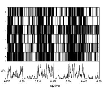
Figure 1: Three days activity plot obtained from six laboratory animals (“A” trough “F”) exposed to a cycle of 12 hours of light (6AM-6PM) and darkness (6PM-6AM), individually housed and continuously monitored by an infrared device scanning the field at a rate of 1 Hz. The bottom timeseries, depicts the group average activity $\langle R\rangle$, computed with a binwidth of 1 min and normalized.

Animal’s movement was monitored with infrared activity-meters, able to scan each rodent housing cage and to report, at a frequency of 1 Hz, animal movements even in absence of locomotion. Given the sensor’s sensitivity the detection includes even minute head motion, grooming, etc. An example of the recording for the first three days is plotted in Fig. 1, where changes from activity to immobility, and viceversa, are marked by a vertical bar, with a resolution of 1 s. In the bottom plot of Fig. 1, we also show the group average of the activity rate $R$, which is a coarse graining of the raw data, exhibiting the well known circadian rhythmicity.

Our interest here focuses exclusively on understanding the dynamics of the irregular fluctuations and not on the circadian periodicity.

III Statistical properties

The spatial and temporal resolution of our experimental setting is such that, from the original (binary) data recorded, we can precisely estimate the duration of motion (sequences of 1’s) and immobility (sequences of 0’s) episodes. Thus, the animal motor activity can be interpreted as a point process where the beginning of a motion event occurs at a definite discrete time $t_{i}$. The point process can be then specified by the sequence of event times $t_{i}$ or, alternatively, by the series of increments (or inter-event intervals) $\tau_{i}=t_{i+1}-t_{i}$. A typical plot of the $\tau$-series is presented in Fig. 2. It is evident that, beyond the circadian rhythmicity, clustering or bursts of activity occur.

Figure 2: Inter-event time $\tau_{i}$ as a function of the event number $i$. (Data from animal A.)

In order to characterize this point process we will first consider the $\tau$-series, obtaining its distribution and correlation structure. Next, rates of events will be inspected. Finally, the statistics of event’s counts thurner as a function of observation times will be described.

III.1 Inter-event intervals

Fig. 3 shows the estimation of the probability density $P(\tau)$ through the relative frequency of occurrence of inter-event times. It was computed over the nine-day activity (binary) recordings, for each one of the six animals. We have overimposed the plots from all the animals to demonstrate the robustness of the results. It can be clearly seen that, from few seconds to several thousands seconds (about 1 hour), the distribution of inter-event times decays as a power-law (with exponent $\mu$ falling within the interval $1.75\pm 0.5$ for all six animals).

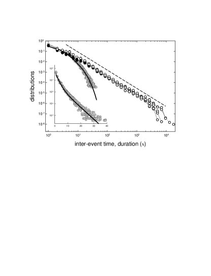
Figure 3: Normalized distributions of: inter-event times $\tau$ (empty symbols), duration of motion episodes (gray symbols) and duration of immobility periods (black symbols), computed from nine days of continuous recording. Symbols joined by dotted lines correspond to the results from each one of the six animals. The solid lines correspond to a double exponential fit (with characteristic times of the order of 1 s and 4 s). The dashed line, drawn for comparison, has slope -1.75. Inset: representation of the distribution of motion episodes in log-linear scale. Statistics computed individually for each of the six animals and plotted overimposed

In contrast, the distribution of duration of motion episodes do possess a characteristic timescale (see also Fig. 3). It can be described by a superposition of two exponentials with characteristic times of the order of 1 s and 4 s, close to the smaller data resolution and to the average duration of motion episodes, respectively. Let us note that, for human (arm) motor activity data, instead of two exponentials, a stretched exponential fit was reported nakamura .

Meanwhile, quiescence intervals are also power-law distributed with exponent $\mu$. Because motion intervals are in average much shorter than quiet ones, then, the statistics of inter-event times is mainly dominated by that of immobility periods, in particular, sharing the same power-law decay. Hence, discrepancies between both histograms are evident for small time intervals only (see Fig. 3). For comparison, let us note that, for the power-law exponent of the cumulative histogram of inactivity periods of human (arm) motor activity, the values $0.92$ (control) and $0.74$ (depressed individuals), with about 10% relative error, have been reported nakamura .

Identical distributions to those exhibited in Fig. 3 were obtained when day and night fluctuations were analyzed separately, only differing in the cutoffs, occurring at longer activity (inactivity) intervals, at day (night). Therefore the fundamental statistical features are independent of the level of activity.

To assess correlations, first we computed the spectral density of $\tau$, displayed in Fig. 4, showing that inter-event intervals are not independent. Therefore, the stochastic point process of motor activity can not be considered a renewal one. Because of the relatively small value of the exponent of the $\tau$ power spectrum, we computed also that of the increments, which helps to confirm that it is not white noise. Although not shown, we verified also that motion and quiescent intervals are anticorrelated.

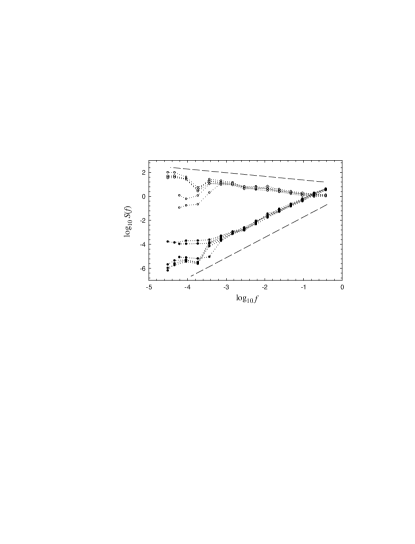
Figure 4: Long-range correlations of inter-event times. Log-log plot of the power spectra for the six series of inter-event intervals (open symbols) and of their increments (filled symbols). Data were logarithmically binned. Here $f$ is in units of the inverse event number. Dashed lines are a guide to the eyes, with slopes $-0.3$ and $1.7$. Notice that, $\alpha=0.3$ and $\beta=1.7$, verify $\alpha=2-\beta$. (Data from six animals.)

III.2 Local rates

By dividing the whole observation time interval in $W$ (nonoverlapping) uniform windows of length $T$ and counting the number of events, $N_{n}$, in each time window $n$, one obtains the series of counts. The cumulative number of events, ${\cal N}(t)=\sum_{n=1}^{m}N_{n}$ vs. time $t=\sum_{n=1}^{m}\tau_{n}$, is shown in Fig. 5(a). One observes that the local rate (local slope) is not constant as in standard Poisson processes. It varies on time, following not only the slowly circadian trend but also other rapidly changing ones.

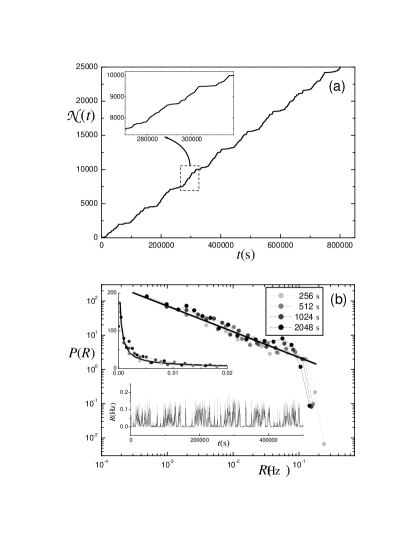
Figure 5: (a) Cumulative number of events as a function of time. A zoom is displayed in the inset. (b) Distribution of local rates $R$ computed over non-overlapping time windows of lengths $T$ indicated on the figure. The solid line corresponds to a power-law with exponent $\gamma=0.75$, drawn for comparison. Upper inset: the same plot in linear scale. Lower inset: timeseries of local rates $R$ for two of the time window lengths considered. (Data from animal A.)

In order to depict more precisely rate inhomogeneities, we estimated local rates $R_{n}$, as being the ratio of $N_{n}/T$. In the scale of half-day, one observes two characteristic mean rates associated to the half-periods of low and high activity levels. However, shorter time windows $T$ reveal a more complex structure of the distribution of rates, that is not simply bimodal but has the shape displayed in Fig 5(b). It follows as a power-law (with exponent $\gamma\simeq 0.75$) with exponential cut-off. The higher probability of small rates leads to longer intervals of immobility. Notice also that there is a range of window lengths for which the distribution of rates remains invariant, a scaling feature typical of a fractal-like process. Besides this scaling property, rates fluctuate in time, as exhibited in the lower inset of Fig. 3(b). Nonhomogeneous Poisson processes with (uncorrelated) stochastic rates have been considered to explain the emergence of scaling in the statistics of inter-event times (see for instance hidalgo ). Since in the present case the inter-event intervals are not independent, such inhomogeneous Poisson processes can be excluded as responsible for this dynamics.

To estimate rate linear correlations, we performed a spectral analysis of the time series of increments $I_{n}=R_{n}-R_{n-1}$. Fig. 6 is a log-log plot of its power spectrum $S(f)$. It is approximately linear on a wide range of biologically relevant temporal scales implying that $S(f)\sim f^{\beta}$, with $\beta\sim 1$. Since $\beta>0$, consecutive values of the process $I$ are negatively correlated, meaning that increases in activity are, on the average, more likely to be followed by decreases and viceversa. Shuffling the timeseries of increments yields white noise. Recalling that $R$ is the integration of $I$, then the spectral density of the original $R$ timeseries decays as $1/f^{\alpha}$ with $\alpha=2-\beta$ Peng93 .

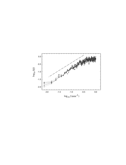
Figure 6: Long-range anticorrelations in the increments $I_{n}$ of activity rates $R_{n}$ computed over 1-min windows. Log-log plot of the power spectra for the six $I$ timeseries (symbols). The dashed line with slope $\beta=1$ indicates the correlations expected for pink noise. (Data from six animals).

III.3 Variance of counts

Common measures for detecting correlations in sequences of counts are the Fano ($FF$) and Allan ($AF$) factors thurner . The former is the ratio of the variance to the mean of the number of events in each time-window, $FF=(\langle[N_{k}]^{2}\rangle-\langle N_{k}\rangle^{2})/\langle N_{k}\rangle$, an index of dispersion of counts. The latter quantifies the discrepancy of counts between consecutive windows, being $AF=(\langle[N_{k+1}-N_{k}]^{2}\rangle)/(2\langle N_{k}\rangle)$. Although related, they reflect different features, therefore we kept track of both of them. In Fig. 7, the two factors are plotted as a function of the length of the counting time window $T$. There is a range where they increase as $T^{d}$. The exponent of $FF$ is $d\in[0.65,0.73]$ (that is $d\simeq\mu-1$, within error bars), for the six laboratory animals, while that of $AF$ is about 0.1 higher. The discrepancy may be due to the fact that $FF(AF)$ tends to the power law from above(below). Their power-law behaviors indicate that the temporal support of the spikes of activity is a fractal-like set with dimension $d$. Shuffling the series of inter-event intervals modifies both factors, mostly by reducing the upper bound of the power-law scaling region. This indicates that the scaling properties are partially due to the distribution of inter-event intervals itself, but also that some correlations are associated with the specific ordering of the intervals.

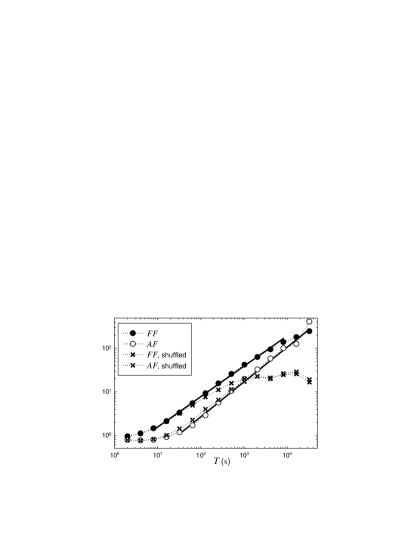
Figure 7: Fano and Allan factors as a function of the counting time-window length $T$. Solid lines are the results of fits giving slopes $d\simeq 0.7$ and $d\simeq 0.8$, respectively. For comparison, the same analysis over the series of shuffled time intervals is also shown. (Data from animal A.)

IV Modeling the dynamics

The observed super-Poissonian behavior discussed in the previous Section points in the direction of a multiplicative or clustering process, where the occurrence of an event increases the probability of a subsequent one teich . A class of clustering Poisson process was introduced by Grüneis gruneis90 , where there is a primary Poisson process triggering the occurrence of a sequences of events (clusters), each following a secondary Poisson process. In each cluster the number $m$ of events is a random variable.

The statistical properties of this two-stage cascade are determined also by the cluster size distribution $p(m)$. A special case of interest in the context of $1/f^{\alpha}$ fluctuations is $p(m)\propto 1/m^{\eta}$, for $m\leq N_{0}$, and null otherwise. For $3/2<\eta<3$, in the limit $N_{0}\to\infty$, it was reported gruneis90 that the exponent of the variance/mean curve is $d\simeq(7-2\eta)/4$ while the exponent of the spectral density is $3-\eta$. If $\eta=2$, $1/f$ noise is obtained and $d=3/4$, which is in good accord with the present outcomes. Although Grüneis et al. clustering Poisson process can reproduce some of the observed scalings, it is not clear how such a cascade process would precisely be originated in the present context.

The same difficulty applies to other fractal or fractal-rate stochastic point processes thurner . Recall also that, for many processes cited in Ref. thurner , solely the distribution of rates is scale-free, while inter-event times present a more trivial statistics. In the present case, however, inter-event times are not only scale-free but also present long-range correlations, indicating non renewal processes.

It is plausible that animal activity is triggered when an internal dynamical state variable reaches some value. Without being too specific, an animal can move to eat when sugar level reaches some low value, for instance. Of course, biological reality will indicate that nothing in the judgement of the state variable nor in the threshold value can be very precise. Therefore, one can imagine a quantity relaxing towards a fluctuating threshold that resets upon crossing it. Variants of this scenario are very common in the the literature where fluctuations are introduced in either the threshold level or in the activation function wing ; schoner ; wagenmakers ; th_model . In particular, we examine here the variant introduced by Davidsen and Schuster th_model , where the threshold fluctuates following a (bounded) Wiener process with diffusion constant $D$. In Fig. 8(a), we present a representative example of the fluctuating threshold $\Theta$ and the relaxation dynamical variable $V$ as functions of time.

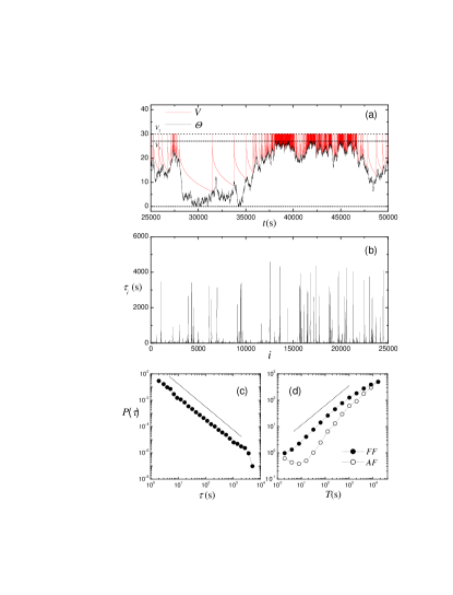
Figure 8: Relaxation toward a fluctuating threshold model. (a) Plots as a function of time of: the threshold $\Theta$ (black line), that fluctuates diffusively (with coefficient $D$) between the levels 0 and $V_{1}$ (dashed lines); the dynamical variable $V$ (thin red line) that describes the relaxation from the excited level $V_{2}$ (dotted line) down to the threshold and is characterized by amplitude $K$ and exponent $\kappa$. (b)-(d) Results of simulations performed up to time $10^{6}$ in units that correspond approx. to 1 s of real time. Model parameters are $(V_{1},V_{2},D,K,\kappa)=(27,30,0.04,3.0,0.25)$. (b) Series of inter-event intervals. (c) Distribution of inter-event times. Dotted line indicates $\mu=1.75$. (d) Fano and Allan factors vs. counting window length $T$. Dotted line corresponds to $d=0.7$.

Fig. 8(b)-(d) show the model dynamics. The distribution of inter-event times depends on the specific shape of the decay of $V(t)$, the relaxation process. If the decay has the shape $V(t)=V_{2}-K(t-t_{last})^{\kappa}$, where $t_{last}$ is the time of the previous adjacent trigger, then the power-law distribution of inter-event times has exponent $\mu=2-\kappa$ th_model . In particular $\kappa=0.25$, yields $\mu=1.75$ close to the observed values, and as soon as $\kappa$ approaches zero (abrupt decay), the exponent can increase up to a value slightly smaller than 2. This relaxation ruled by $\kappa$ might explain the observation in Ref. nakamura of $\mu\sim 1.7$ in depressed individuals and $\mu\sim 1.9$ in control ones.

Besides the inter-event time distributions, the other main correlation features seen in the data are reproduced as displayed by the $FF$ and $AF$ measures (notice, though, the relatively larger dip for short $T$ in the $AF$). It is known that the model dynamics yields $1/f$ spectral properties th_model . We have verified (not shown) that the inter-event times are power-law correlated and that the distribution of rates is scale free, as observed for real data, although the exponents are different for the chosen set of parameter values.

Overall, this simple model is able to reproduce the observed phenomenology and it is known to be robust under the addition of noise over the activation signal th_model . Finally, the duration of individual events could also be incorporated easily into the model by an additional integration process consistent with the observed statistics.

V Final observations

In summary, the results show that animal motion is scale free in all of the relevant statistics analyzed and that the scaling is introduced by the length of the inactivity pauses as well as its specific ordering.

These results are robust for all animals studied, and invariant when day and night data are analyzed separately. While motion episodes do possess a definite timescale and are basically exponentially distributed, the distribution of inter-event intervals are scale-free over many timescales, from a few up to thousands of seconds. Scaling is also demonstrated in the the rates of occurrence, rejecting a non-homogeneus Poisson process as responsible for the dynamics.

At even longer time scales than the ones considered here, many human actions exhibit also bursty patterns, in which short time intervals of intensive activity are (frequently) separated by long gaps without activity barabasi . In that case, the power-law tails of inter-event distributions have been attributed to queuing processes (where the queue represents the tasks on a priority list). Depending on the dynamics of the priority list, different classes of universality can emerge barabasi . Probably this is not the case in the present experiments, where more likely, an elementary physiological and/or environmental mechanism is behind.

Some of the scale-free properties here observed, have been reported before for human motor activity data as well hu2004 ; amaral . The quantitative aspects for the scaling laws were reported to remain unchanged under usual daily activities or periodic scheduled work. These observations were consistent with earlier results from the study of timeseries of heartbeat intervals Peng93 ; Meesmann1 ; Meesmann2 from healthy humans. Then, it have prompted the suggestion of multi-scale physiological mechanisms as responsible for the presence of long-term correlated dynamics hu2004 . Other related approaches bak1 consider that animal motion could be visualized as the output of a large nonlinear dynamical system (e.g., the brain-body-environment ensemble) whose repertoire includes the kind of dynamics observed in these experiments. Finally, the possibility that the complexity of the environment in itself influences animal behavior needs to be carefully considered foraging .

The specific mechanism discussed here, involving a fluctuating-threshold controlled dynamics is biologically plausible, and not only can replicate observed features of the statistical structure of rat motor activity, but with appropriate modifications can be used to provide insights about the long-term rhythms alterations observed on individuals with mood disorders, depression and other neurological disorders, such as chronic pain.
Acknowledgements: DRC acknowledges support by NIH NINDS of USA (Grants NS58661). CA acknowledges Northwestern University for the kind hospitality and Brazilian agencies CNPq and Faperj for partial financial support.

References

- (1) K. Hu, P.C. Ivanov, Z. Chen, M.F. Hilton, H.E. Stanley, S.A. Shea, Physica A 337, 307-318 (2004).
- (2) T. Nakamura, K. Kiyono, K. Yoshiuchi, R. Nakahara, Z.R. Struzik, Y. Yamamoto, Phys. Rev. Lett. 99, 138103 (2007).
- (3) L.A.N. Amaral, et al., Europhys. Lett. 66, 448-454 (2004); K. Ohashi, G. Bleijenberg, S. van der Werf, J. Prins, L.A.N. Amaral, B.H. Natelson, Y. Yamamoto, Methods Inf. Med. 43, 26-29 (2004).
- (4) A. Vazquez, J.G. Oliveira, Z. Deszso, K.I Goh, I. Kondor, A.-L. Barabasi, Phys. Rev. E 73, 036127 (2006); A.-L. Barabasi, Nature 435, 207 (2005).
- (5) Experiments conducted at Northwestern University according with Animal Care and Use Committee regulations.
- (6) S. Thurner, S.B. Lowen, M.C. Feurstein, C. Heneghan, H.G. Feichtinger, M.C. Teich, Fractals 5, 565-595 (1997).
- (7) C.A. Hidalgo R., Physica A 369, 877 (2006).
- (8) C.-K. Peng, J. Mietus, J.M. Hausdorff, S. Havlin, H.E. Stanley, A.L. Goldberger, Phys. Rev. Lett. 70, 1343-1346 (1993).
- (9) B.E.A. Saleh, M.C. Teich, Proc. IEEE 70, 229-245 (1982).
- (10) F. Grüneis, M. Nakao, M. Yamamoto, Biol. Cybernetics 62, 407-413 (1990); F. Grüneis, Physica A 123, 149-160 (1984); F. Grüneis, H.J. Baiter, Physica A 136, 432-452 (1986).
- (11) A.M. Wing, A.B. Kristofferson, Perception & Psychophysics 13, 455-460 (1973).
- (12) G. Schöner, Brain and Cognition 48, 31-51 (2002), and references therein.
- (13) E.-J. Wagenmakers, S. Farrell, R. Ratcliff, Psychonomic Bulletin & Review 11, 579-615 (2004).
- (14) J. Davidsen, H.G. Schuster, Phys. Rev. E 65, 026120 (2002).
- (15) C. Braun, P. Kowallik, A. Freking, D. Hadeler, K.-D. Kniffki, M. Meesmann, Am. J. Physiol. Heart Circ. Physiol. 275, H1577-H1584 (1998).
- (16) M. Meesmann , J. Boese, D.R. Chialvo, P. Kowallik, W.R. Bauer, W. Peters, F. Grüneis, K.-D. Kniffki, Fractals 1, 312-320 (1993).
- (17) P. Bak, How Nature works. (Oxford University Press, Oxford UK 1997).
- (18) D. Boyer, G. Ramos-Fernandez, O. Miramontes, J. L. Mateos, G. Cocho, H. Larralde, H. Ramos, F. Rojas, Proc. of the Royal Society of London B: Biological Sciences 273, 1743-1750 (2006). Also as http://xxx.lanl.gov/abs/q-bio.PE/0601024.