High-Redshift SDSS Quasars with Weak Emission Lines

Abstract

We identify a sample of 74 high-redshift quasars ($z>3$) with weak emission lines from the Fifth Data Release of the Sloan Digital Sky Survey and present infrared, optical, and radio observations of a subsample of four objects at $z>4$. These weak emission-line quasars (WLQs) constitute a prominent tail of the Ly$\alpha$+N v equivalent width distribution, and we compare them to quasars with more typical emission-line properties and to low-redshift active galactic nuclei with weak/absent emission lines, namely BL Lac objects. We find that WLQs exhibit hot ($T\sim 1000$ K) thermal dust emission and have rest-frame 0.1–5 $\mu$m spectral energy distributions that are quite similar to those of normal quasars. The variability, polarization, and radio properties of WLQs are also different from those of BL Lacs, making continuum boosting by a relativistic jet an unlikely physical interpretation. The most probable scenario for WLQs involves broad-line region properties that are physically distinct from those of normal quasars.

1. Introduction

The optical and ultraviolet (UV) spectra of type 1 quasars are characterized by a blue power-law continuum and strong, broad permitted emission lines with $\textnormal{FWHM}=1000$–$20,000$ km s^-1. These lines are thought to originate in photoionized gas located $\sim 10^{16\textnormal{\scriptsize{--}}18}$ cm from the central black hole, with differential gas velocities producing Doppler-broadened line profiles (e.g., Peterson, 1997; Krolik, 1999). This gas may be confined to individual clouds outside of the accretion disk or it may be related to the accretion disk itself, perhaps as part of a disk wind (e.g., Emmering et al., 1992; Murray et al., 1995).

Observationally, the strongest of these emission lines, in terms of both flux and equivalent width (EW), is Ly$\alpha$ $\lambda 1216$. Results from UV spectra at $z<2$ and optical spectra at $z>2$ (e.g., Schneider et al., 1991; Francis et al., 1993; Osmer et al., 1994; Warren et al., 1994; Zheng et al., 1997; Brotherton et al., 2001; Dietrich et al., 2002) show that the rest-frame EW of Ly$\alpha$+N v $\lambda 1240$ is typically 50–110 Å. These results, however, are based on small numbers of sources, with tens to hundreds of quasars per study. The Sloan Digital Sky Survey (SDSS, York et al., 2000) has substantially increased the available spectroscopic sample of high-redshift quasars; more than $5000$ quasars have been discovered at $z>3$ (Schneider et al., 2007), extending all the way to $z=6.42$ (Fan et al., 2003). The SDSS quasar selection algorithm at these redshifts (Richards et al., 2002a) is based largely on the red colors produced by the Lyman break ($\lambda_{\scriptsize{\textnormal{rest}}}=912$ Å) and the onset of the Ly$\alpha$ forest ($\lambda_{\scriptsize{\textnormal{rest}}}=1216$ Å). It is sensitive to quasars with bright UV continua, without a strong dependence on emission-line strength (Fan et al., 2001), and a small fraction of high-redshift quasars has been found with very weak or absent Ly$\alpha$ emission (e.g., Fan et al., 1999; Anderson et al., 2001; Collinge et al., 2005; Fan et al., 2006).

The first weak-emission line quasar (WLQ) found at high redshift was SDSS J153259.96-003944.1 ($z=4.62$, Fan et al., 1999, hereafter SDSSJ1532). Its flat continuum and lack of emission lines suggested that it could be the highest-redshift BL Lac object ever found, but its paucity of radio flux, X-ray flux, and optical polarization were inconsistent with the BL Lac hypothesis. The spectra of classical BL Lacs lack emission lines because their continuum emission is relativistically boosted by a jet along the line of sight, and they are usually radio-loud, X-ray-loud, and highly polarized (e.g., Urry & Padovani, 1995). The nature of SDSSJ1532 was left as an open question.

Subsequently, two additional WLQs, SDSS J130216.13+003032.1 ($z=4.47$, hereafter SDSSJ1302) and SDSS J144231.72+011055.2 ($z=4.51$, hereafter SDSSJ1442), were identified by Anderson et al. (2001), and the strong radio and X-ray emission of the latter (Schneider et al., 2005; Shemmer et al., 2006) indicated that its continuum could be moderately beamed. In a sample of optically selected BL Lac candidates, Collinge et al. (2005) found seven sources at $z>2.7$, including three radio sources and one X-ray source (Schneider et al., 2003). The highest-redshift WLQ, SDSS J133550.81+353315.8 at $z=5.93$, was discovered by Fan et al. (2006), who discussed whether it could be a strongly lensed galaxy, a BL Lac object, or a quasar with a very weak emission-line region.

Further insight into the nature of WLQs has been gained from pointed X-ray observations with Chandra. Vignali et al. (2001) presented observations of SDSSJ1532, while Shemmer et al. (2006) presented deeper data for SDSSJ1532, as well as observations of SDSSJ1302, SDSSJ1442, and SDSS J140850.91+020522.7 ($z=4.01$, hereafter SDSSJ1408); Shemmer et al. (2006) discussed whether the weak emission lines could be due to continuum boosting or a deficit of line-emitting gas. Shemmer et al. (2009) presented deeper data for SDSSJ1302 as well as observations of eight additional WLQs at $z>2.7$; they also compared the optical, X-ray, and radio properties of WLQs to those of BL Lacs, and discussed whether WLQs could be extreme quasars with high accretion rates. They found that WLQs are weaker than BL Lacs at radio and X-ray wavelengths relative to the optical, but that there is no evidence of steep hard X-ray spectra characteristic of high accretion rates.

This paper extends the study of WLQs to the full high-redshift ($z>3$) sample that has been discovered by the SDSS, and uses a rich, multiwavelength data set for a subsample of four WLQs at $z>4$ to test the available hypotheses regarding their nature. In Section 2, we measure EW(Ly$\alpha$+N v) for each $z>3$ quasar in the Fifth Data Release Quasar Catalog (Schneider et al., 2007), select quasars with EW values $>3\sigma$ below the mean of the distribution, and compare their properties to those of the general high-redshift quasar population. Sections 3, 4, and 5 then present results from an extensive observational campaign focusing on the WLQs SDSSJ1302, SDSSJ1408, SDSSJ1442, and SDSSJ1532. These data include Spitzer 3.6–24 $\mu$m mid-infrared (mid-IR) photometry and near-IR photometry in $J$, $H$, and $K_{s}$ bands that are compared to the spectral energy distributions (SEDs) of typical quasars (Section 3); multiple epochs of optical spectroscopy and $i$-band photometry (in addition to the available SDSS data) that constrain the line and continuum variability of WLQs (Section 4); and optical imaging polarimetry along with Very Large Array (VLA) radio continuum observations at $L$ and $C$ bands that test for the presence of synchrotron emission from a relativistic jet (Section 5). We discuss the implications of our results and the connection to lower-redshift quasars with weak emission lines (e.g., McDowell et al., 1995; Leighly et al., 2007a) in Section 6, and we summarize and conclude in Section 7.

We assume a cosmology with $\Omega_{\Lambda}=0.7$, $\Omega_{M}=0.3$, and $H_{0}=70$ km s^-1 Mpc^-1. All quoted emission-line EWs are in the rest frame of the quasar.

Figure 1.— Spectra of six $z>3$ quasars exhibiting a range of redshifts, Ly$\alpha$+N v emission-line EWs, continuum spectral slopes, and S/N. The wavelength corresponding to $\lambda_{\scriptsize{\textnormal{rest}}}=1216$ Å is marked by a dotted line in each spectrum. The objects in the second and fifth panels are WLQs.

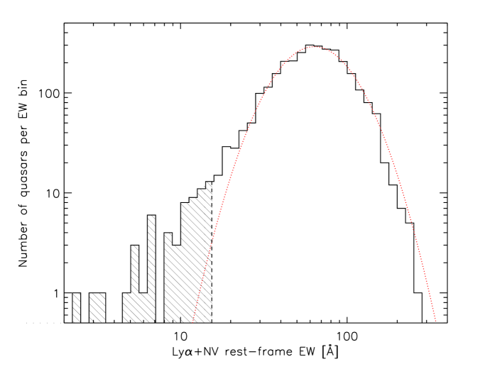
Figure 2.— Distribution of rest-frame Ly$\alpha$+N v EWs for the sample of 3058 $z>3$ non-BAL quasars described in Section 2. The dotted red line shows the best-fit log-normal distribution, with a mean EW of $63.6$ Å and a $1\sigma$ range of $39.6$–$101.9$ Å. The fit is a reasonable description of the data above $\textnormal{EW}=20$ Å, but there is a prominent tail toward low EW values. The dashed line and the hashed section of the histogram indicate our WLQ definition.

Figure 3.— Composite spectra of $z>3$ quasars in different EW(Ly$\alpha$+N v) bins. The wavelengths of Ly$\alpha$ and C iv are marked by dotted lines. Top panel: Composite for 428 quasars with EW $>1\sigma$ above the mean ($\textnormal{EW}>101.9$ Å). Second panel: composite for 1038 quasars with EW between the mean and $1\sigma$ above it ($63.6~{}\textnormal{\AA}<\textnormal{EW}<101.9$ Å). Third panel: composite for 1000 quasars with EW between the mean and $1\sigma$ below it ($39.6~{}\textnormal{\AA}<\textnormal{EW}<63.6$ Å). Fourth panel: composite for 536 quasars with EWs between $1\sigma$ and $3\sigma$ below the mean ($15.4~{}\textnormal{\AA}<\textnormal{EW}<39.6$ Å). Fifth panel: composite for 56 WLQs with EW $>3\sigma$ below the mean ($\textnormal{EW}<15.4$ Å). Bottom panel: composite for the subset of 32 WLQs that do not exhibit significant C iv emission or PDLA absorption (see Table 2). There is a trend for the Ly$\alpha$/N v ratio to decrease toward lower EWs.

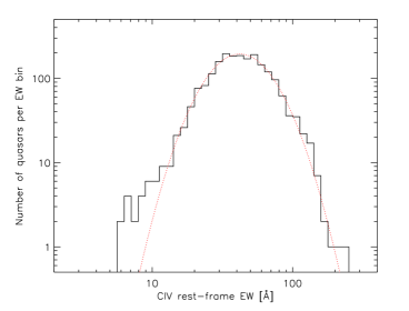
Figure 4.— Distribution of C iv EWs for 2035/3058 quasars from Figure 2 measured from emission-line fits performed by Shen et al. (2008). The dotted red line shows the best-fit log-normal distribution, with a mean EW of $41.9$ Å and a $1\sigma$ range of $26.1$–$67.4$ Å. Objects with the weakest C iv lines are not included because accurate EWs could not be determined.

2. The Weak Emission-Line Quasar Sample

The SDSS Fifth Data Release Quasar Catalog includes $77,429$ objects and covers an area of 5740 deg² (Schneider et al., 2007). The 5374 quasars at $z>3$ are selected down to a magnitude limit of $i=20.2$ (Richards et al., 2006a). The SDSS spectra have wavelength coverage $\lambda=3800$–$9200$ Å and resolution $R\sim 2000$. In Figure 1, we show six spectra exhibiting a range of redshifts, emission-line EWs, continuum spectral slopes, and signal-to-noise ratios (S/Ns), including two WLQs.

For each spectrum, we fit a power law of the form $f_{\lambda}=C\times\lambda^{\beta}$ to regions of the continuum that are generally uncontaminated by emission lines (1285–1295, 1315–1325, 1340–1375, 1425–1470, 1680–1710, 1975–2050, and 2150–2250 Å). We then integrate the flux above the power-law continuum between $\lambda_{\scriptsize{\textnormal{rest}}}=1160$ Å and $\lambda_{\scriptsize{\textnormal{rest}}}=1290$ Å to determine emission-line flux and EW. This region includes the Ly$\alpha$ $\lambda 1216$, N v $\lambda 1240$, and Si ii $\lambda 1263$ emission lines, so we measure the strength of a blended emission feature that is dominated by the Ly$\alpha$ and N v components. The median S/N of the spectra integrated over this wavelength region is $140$ for line$+$continuum and $95$ for the continuum.

The EW(Ly$\alpha$+N v) measurements for all 5374 quasars are given in Table 1. The typical statistical uncertainty of each measurement is $\sim 1$–2 Å. There is also a systematic uncertainty in the placement of the continuum level, which depends on the wavelength regions chosen for the continuum fit. Visual inspections show that the fits accurately describe the data, and while the EWs of individual objects do change slightly ($\sim 10\%$) if different wavelength regions are used to fit the continuum, the aggregate results are quite similar. An important caveat is that our method underestimates the intrinsic line strength when strong intervening absorption is present. Some studies (e.g., Dietrich et al., 2002) interpolate across Ly$\alpha$ forest absorption features and fit the intrinsic emission-line profile, but this requires an accurate determination of the absorption systems along the line of sight to each quasar and is difficult without high-S/N data at higher spectral resolution. The effects of Ly$\alpha$ forest absorption are discussed further below and in Section 2.1.3. In addition, there is a break in the quasar continuum near $\lambda_{\scriptsize{\textnormal{rest}}}=1100$ Å (e.g., Zheng et al., 1997; Shang et al., 2005), so our power-law continuum fit at $\lambda_{\scriptsize{\textnormal{rest}}}>1285$ Å may slightly overestimate the continuum flux at Ly$\alpha$ and therefore underestimate the strength of the emission feature.

We restrict our analysis to the $3979$ sources that were identified as primary quasar targets by the final algorithm given by Richards et al. (2002a). These objects have the uniform selection flag set in the Schneider et al. (2007) catalog and constitute a statistical color-selected sample. We additionally exclude 915 broad-absorption line (BAL) quasars from the catalogs of Trump et al. (2006) and Gibson et al. (2009), as well as six objects flagged by visual inspection as having either BAL-like absorption or missing data in the Ly$\alpha$ region. The final sample includes a total of 3058 quasars.

The distribution of Ly$\alpha$+N v rest-frame EWs for this sample is shown in Figure 2. The median and mean of the measured values are 62.3 Å and 67.6 Å, respectively. The distribution is well described by a log-normal function with best-fit parameters $\langle\log\textnormal{EW}\rangle=1.803$ and $\sigma(\log\textnormal{EW})=0.205$, corresponding to a mean of $63.6$ Å and a $1\sigma$ range of 39.6–101.9 Å. However, there is a prominent tail toward small values. If the $\log$(EW) values were indeed distributed like a Gaussian, where the $3\sigma$ range encompasses 99.73% of the curve area, we would expect to find $\sim 4$ objects beyond this range ($\textnormal{EW}=15.4$–261.9 Å) at each end. Instead we find none at the high end and 56 at the low end, and we define our sample of WLQs to be these 56 objects with $\textnormal{EW}<15.4$ Å. This WLQ definition is more inclusive than the $\textnormal{EW}<10$ Å definition adopted by Shemmer et al. (2009), but the precise cutoff between WLQs and “normal” quasars is somewhat arbitrary; our goal is simply to select the sources with extreme EWs that exist beyond what would be expected from a simple log-normal distribution.

To illustrate the spectroscopic properties of WLQs relative to the rest of the quasar sample, we construct composite spectra in bins of EW(Ly$\alpha$+N v) and present them in Figure 3. These composite spectra span the range $\lambda_{\scriptsize{\textnormal{rest}}}=800$–1800 Å and are constructed following the method of Fan et al. (2004); each spectrum is normalized based on its flux at $\lambda_{\scriptsize{\textnormal{rest}}}=1450$ Å and the average of all spectra is computed. We use five EW bins: (1) EW $>1\sigma$ above the mean, 428 objects; (2) EW between the mean and $1\sigma$ above it, 1038 objects; (3) EW between the mean and $1\sigma$ below it, 1000 objects; (4) EW between $1\sigma$ and $3\sigma$ below the mean, 536 objects; and (5) EW $>3\sigma$ below the mean, 56 objects. In the first three composite spectra, the red side of the Ly$\alpha$+N v blend (dominated by N v) is nearly identical, but the blue side (dominated by Ly$\alpha$) steadily decreases in strength; while in the fourth spectrum, the peak flux shifts redward of $\lambda_{\scriptsize{\textnormal{rest}}}=1216$ Å as the N v component begins to dominate. This trend continues in the WLQ composite, where the 1216 Å flux actually drops below the (unabsorbed) continuum level. This extreme behavior is driven by a handful of WLQs with strong absorption features, and in fact 15/56 WLQs are included in the Prochaska et al. (2008) catalog of proximate damped Ly$\alpha$ absorbers (PDLAs, $\Delta v<3000$ km s^-1, $N_{H}>2\times 10^{20}$ cm^-2). In the bottom panel, we exclude these WLQs whose weak Ly$\alpha$+N v lines can be explained by absorption rather than intrinsic weakness, as well as 10 additional WLQs that exhibit $\textnormal{EW}(\textrm{C}~{}\textsc{iv})>10$ Å (these sources are flagged in Table 2). The resulting WLQ composite spectrum has flux roughly equal to the continuum level near Ly$\alpha$ $\lambda$1216, a weak emission feature near N v $\lambda$1240, and a negligible bump near C iv $\lambda$1549.

There is also a trend for the continuum luminosity to increase in the lower EW bins. The median continuum luminosity for the whole sample is 41% larger than the median for sources in the highest EW bin and 39% smaller than the median for WLQs. This trend is consistent with the Baldwin effect (the observed anti-correlation between C iv EW and quasar luminosity; Baldwin, 1977).

We select the WLQ sample based on extreme Ly$\alpha$+N v EWs rather than C iv because the former line is stronger, and therefore readily detected even at low S/N, and observable at the highest redshifts ($z>4.9$). However, we do compile C iv EWs measured from emission-line fits performed by Shen et al. (2008). These values are presented in Table 1, and their distribution is shown in Figure 4. For the 2035/3058 quasars in our final sample where the Shen et al. (2008) fits yield secure C iv EWs, the best-fit log-normal distribution has parameters $\langle\log\textnormal{EW}\rangle=1.622$ and $\sigma(\log\textnormal{EW})=0.206$ (mean 41.9 Å, $1\sigma$ range 26.1–67.4 Å), and the median EW ratio (Ly$\alpha$+N v)/C iv is 1.53. This ratio is smaller than what has been reported in previous studies (e.g., Schneider et al., 1991; Osmer et al., 1994; Brotherton et al., 2001; Vanden Berk et al., 2001; Dietrich et al., 2002), which tend to find larger EW(Ly$\alpha$+N v) and smaller or comparable EW(C iv) values. As mentioned above, our method underestimates the intrinsic strength of Ly$\alpha$+N v emission when strong Ly$\alpha$ forest absorption is present, and the Shen et al. (2008) fits overestimate EW(C iv) when strong Fe ii emission mimics a broad Gaussian component of the C iv profile; but our results for both lines are nonetheless within the range of literature values (e.g., Francis et al., 1991). Also, early studies (e.g., Schneider et al., 1991; Osmer et al., 1994) were biased toward more luminous quasars, so their lower EW(C iv) values could be explained by the Baldwin effect. There is no information about objects with the weakest C iv lines in Table 1 or Figure 4 because accurate EWs could not be measured from the Shen et al. (2008) fits; in fact, 34/56 WLQs and all objects with $\textnormal{EW}(\textrm{C}~{}\textsc{iv})<6$ Å are not included.

2.1. Sample Properties

To investigate the nature of the low-EW tail of the distribution, in this section we compare several properties of WLQs to those of the general $z>3$ quasar population. We perform this analysis on all 56 WLQs in the uniform sample and on the subset of 31 WLQs with no C iv or PDLA flags (see above and Table 2); the results are insensitive to the choice of sample, and we quote values for the full uniform sample.

2.1.1 Emission-line and Continuum Properties

In addition to EW, our continuum fits to the SDSS spectra yield values of Ly$\alpha$+N v emission-line flux, continuum flux, and continuum spectral slope for each source. We find that the emission-line luminosities of WLQs are all at the low end of the distribution for normal $z>3$ quasars (28/56 WLQs are in the bottom 1%, 44/56 are in the bottom 5%, and all are in the bottom 26%); by the Kolmogorov–Smirnov (K-S) test, the probability that the two samples are drawn from the same parent distribution is $p=4\times 10^{-31}$. The median line luminosity for WLQs is a factor of $3.8$ lower than the median for normal quasars, indicating that Ly$\alpha$ is weak in an absolute sense, rather than just relative to the continuum. As mentioned above, the continuum luminosities for WLQs are somewhat larger on average than those for normal quasars, but their continuum slopes are quite similar. We find median values of $\alpha=-0.54$ and $\alpha=-0.52$ for normal quasars and WLQs, respectively, and the K-S test gives a probability $p=0.20$ that the distributions are the same.

2.1.2 Radio Flux

We also investigate the radio properties of WLQs using data from the Faint Images of the Radio Sky at Tweny cm (FIRST) survey (Becker et al., 1995). A search of the catalog (White et al., 1997) within $2\arcsec$ of each quasar yields 147 detections and 2809 upper limits; 102 quasars, including four WLQs, are not covered by the FIRST footprint. We find that the radio-detection fraction is $4.9$% (142/2904) for normal quasars and 10% (5/52) for WLQs. This difference is not significant; given the radio-detection fraction of normal quasars, the binomial distribution gives a $11\%$ chance of having five or more detections in a sample of 52. If we relax the uniform selection criterion described above and include all non-BAL quasars, the radio fraction increases to 6.1% (233/3811) for the general population and to $21$% (15/70) for WLQs. This increase, which is especially prominent for WLQs, is due to the fact that FIRST sources were targeted for spectroscopy by the SDSS even if their optical colors did not meet the final quasar-selection criteria. Assuming a 6.1% detection probability, the chance of having 15 or more detections in a sample of 70 is only $0.002$%.

A more relevant quantity than the radio detection fraction is the radio-loudness parameter $R$, which is defined as the ratio of radio to optical flux density. We adopt the definition used by Jiang et al. (2007), $R=f_{\nu}(6~{}$cm$)/f_{\nu}(2500~{}$Å$)$. We calculate the rest-frame 6 cm flux density from the observed 20 cm flux density assuming a power-law slope $\alpha_{r}=-0.8$, and we calculate the rest-frame 2500 Å flux density from the observed $z$ band ($\lambda=8931$ Å) flux density assuming a power-law slope $\alpha_{o}=-0.5$. We find that 3.2% (92/2904) of normal $z>3$ quasars and 6% (3/52) of WLQs have $R>100$, while $>4.6$% (133/2904) and $>10$% (5/52) have $R>10$. The latter fractions are lower limits because the FIRST detection threshold, typically $\sim 1$ mJy, is only deep enough to constrain $R<10$ for the optically brightest sources ($\sim 15$% of the sample). Again, including all non-BAL quasars changes the $R>10$ fraction to $>5.9$% (224/3811) and $>21$% (15/70), and the $R>100$ fraction to 4.1% (156/3811) and 7% (5/70).

To compare the distributions of $R$ values statistically, given that most values are upper limits (i.e., the distributions are heavily censored), we use the survival analysis software package ASURV Rev 1.3 (Lavalley et al., 1992), which implements the methods presented in Feigelson & Nelson (1985). We perform the Gehan, logrank, and Peto-Prentice two-sample tests. In the uniformly selected sample, these tests give probabilities $p=0.097$, $p=0.145$, and $p=0.147$ that the WLQs and normal $z>3$ quasars have the same distribution of radio loudness. If the uniform-selection criterion is dropped (i.e., all non-BAL quasars are included), these probabilities drop to $p=1\times 10^{-4}$, $p=2\times 10^{-6}$, and $p=8\times 10^{-6}$. Thus, there is no evidence of a difference in radio properties between WLQs and normal quasars among the sources that were selected for spectroscopy solely on the basis of optical colors. However, the use of FIRST data to identify SDSS spectroscopic targets selects a larger fraction of WLQs; of the non-BAL quasars at $z>3$ with FIRST detections, $6.0$% (15/248) have $\textnormal{EW}(\textrm{Ly}\textsc{$\alpha$}+\textrm{N}~{}\textsc{v})<15.4$ Å. This may be because radio selection is not biased against quasars with weak Ly$\alpha$ emission, while color selection at $z<4$ is biased (see Section 2.1.3).

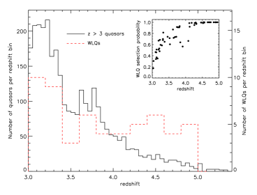
Figure 5.— Redshift distributions of normal $z>3$ quasars (solid black line, bin size $\Delta z=0.05$) and WLQs (dashed red line, bin size $\Delta z=0.20$). The two distributions diverge at $z\sim 4.2$, with WLQs appearing to be more common at higher redshift. The inset panel shows the selection probability for each WLQ (see Section 2.1.3), indicating that weak-lined sources are more likely to be selected at higher redshift. The increased opacity of the IGM near $\lambda_{\scriptsize{\textnormal{rest}}}=1216$ Å at higher redshift is also likely to bias EW measurements toward lower values.

2.1.3 Redshift Distribution

The redshift distributions of normal $z>3$ quasars and WLQs are shown in Figure 5. The two distributions diverge at $z\sim 4.2$, with WLQs constituting $1.3$% ($36/2737$) of the quasar population below this redshift and $6.2$% ($20/321$) above it. The redshifts measured for individual WLQs can be uncertain by as much as $\delta z=0.1$ because of their weak lines (see Section 4.3), but this does not affect the result that WLQs are a larger fraction of the observed quasar population at higher redshift. The typical Ly$\alpha$+N v EW for normal quasars at $z>4.2$ is also lower than for lower redshift quasars, with median values $46.4$ Å and $63.8$ Å, respectively. The greater incidence of lower EW objects at higher redshift could be caused either by selection effects or by some differential physical process (see below). To investigate the former hypothesis, we calculate the selection probability of each WLQ based on its redshift, $i$-band luminosity, spectral slope, and Ly$\alpha$ emission-line EW using the method of Fan et al. (2001) and Richards et al. (2006a). Using a distribution function of H i absorption, we simulate 200 spectra, compute $ugriz$ magnitudes including photometric errors, and apply the quasar-selection criteria. The results are shown in the inset of Figure 5. We find that the selection probabilities of individual WLQs generally increase with redshift, with average probabilities of $p=0.53$ at $z<3.5$ and $p=1.0$ at $z>4.5$. This redshift-dependent selection can be explained by the fact that absorption by the Ly$\alpha$ forest and Lyman Limit Systems (LLSs) equalizes the colors of higher-redshift quasars, independent of their emission line properties (see Section 1). There is also significant dependence on the luminosity and spectral slope, as well as emission-line EW, at each redshift (e.g., Fan et al., 2001, see their Figure 5), but the general result is that WLQs are easier to select at higher redshift. The fact that the observed WLQ fraction is $\sim 6$% in samples that are unbiased with respect to emission-line strength (e.g., FIRST-detected quasars, quasars at $z>4.2$) implies that the intrinsic WLQ fraction may be significantly higher than the $\sim 1$% inferred from the full SDSS sample.

In addition to affecting the colors of WLQs, and thus their likelihood of selection, absorption by the Ly$\alpha$ forest can also affect the Ly$\alpha$ emission line itself, pushing objects toward lower EWs at higher redshift. To have a measurable effect, the absorbing material must be located in close proximity to the quasar, as is clearly the case for 11 WLQs that have PDLAs. However, there is no evidence to suggest that PDLAs, which are generally associated with galaxies in the environment of the quasar (e.g., Møller et al., 1998; Ellison et al., 2002; Russell et al., 2006), are more common at higher redshift, and an analysis of the evolution of the intergalactic medium (IGM) opacity at $z>3$ is beyond the scope of this paper. The relevant effect of the Ly$\alpha$ forest effect on the Ly$\alpha$ emission line, though, can be seen in the composite spectrum of $z\sim 6$ quasars (Fan et al., 2004), and it is likely to bias the EW measurements of the highest-redshift sources.

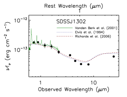
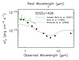
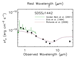
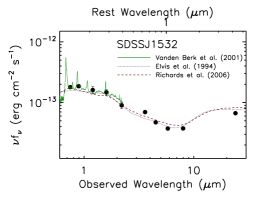
Figure 6.— Observed-frame $0.7-24~{}\mu$m SEDs for four representative WLQs at $z>4$. The data points are SDSS $i$ and $z$ bands; $J$, $H$, and $K_{s}$ bands; Spitzer IRAC 3.6, 4.5, 5.8, and 8.0 $\mu$m; and Spitzer MIPS 24 $\mu$m. For most data points, the error bars are smaller than the dots. Each panel includes the Vanden Berk et al. (2001) quasar composite spectrum scaled to the SDSS data points (green solid line), and the mean quasar composite spectra from Elvis et al. (1994) and Richards et al. (2006b) scaled to all of the data points (blue dotted and red dashed lines, respectively).

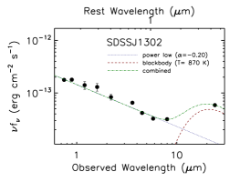
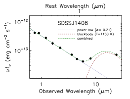
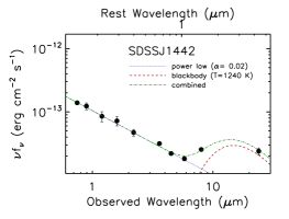
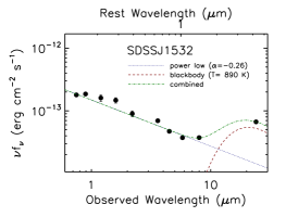
Figure 7.— Data are the same as Figure 6. The dotted blue line shows the best-fit power-law model to the short-wavelength data and the dashed red line shows the best-fit single-temperature blackbody to the longer wavelength data. The dash-dotted green curve is the sum of the two models. Also included are the spectral slope of the power law and the temperature of the blackbody for each source.

3. IR Photometry

This is the first of three sections (Sections 3, 4, 5) that present multiwavelength observations of four $z>4$ WLQs: SDSSJ1302, SDSSJ1408, SDSSJ1442, and SDSSJ1532. These sources were selected early on in the survey to be representative of the handful of WLQs known at the time; their Ly$\alpha$ emission-line strengths range from undetectable (e.g., SDSSJ1532) to weak, but clearly detected (e.g., SDSSJ1442), and two are FIRST radio sources (SDSSJ1408, $R=14$; SDSSJ1442, $R=26$), while the other two have no radio detections. The FIRST-detected sources also have strong Chandra X-ray detections (SDSSJ1408, $\alpha_{ox}=-1.54$; SDSSJ1442, $\alpha_{ox}=-1.42$ Shemmer et al., 2006), while SDSSJ1302 and SDSSJ1532 are X-ray weak ($\alpha_{ox}=-2.08$ and $\alpha_{ox}<-1.90$, respectively; Shemmer et al., 2006, 2009). This section presents Spitzer mid-IR photometry in the 3.6–24 $\mu$m range (Section 3.1) and near-IR photometry in $J$-, $H$-, and $K_{s}$-band (Section 3.2), which we use to construct rest-frame 0.1–5 $\mu$m SEDs of WLQs that can be compared to those of normal quasars (Section 3.3).

3.1. Spitzer Mid-IR Data

We obtained mid-IR photometry for all four sources as part of a Spitzer Space Telescope (Werner et al., 2004) Cycle I General Observer Program (PID 3221). Observations with the IRAC instrument (Fazio et al., 2004) were executed in all four channels ($3.6~{}\mu$m, $4.5~{}\mu$m, $5.8~{}\mu$m, and $8.0~{}\mu$m) with an integration time of 1000 s per channel. Observations with MIPS (Rieke et al., 2004) were obtained in the $24~{}\mu$m channel with integration times of 1400–1500 s.

We begin our analysis of the IRAC data using the Basic Calibrated Data (BCD) products from version S14.0.0 of the Spitzer Science Center software pipeline. The MOPEX software package was used to construct mosaics from the individual frames, which involves background matching between overlapping images and outlier pixel rejection. The native IRAC pixel size of $1.2\arcsec$ yields somewhat undersampled data, so we take advantage of a subpixel dither pattern to interpolate the individual BCD images onto a common grid with a $0.6\arcsec$ pixel scale using the Drizzle algorithm. We perform aperture photometry on the mosaics using the APER task in IDLPHOT. We use $3.6\arcsec$ source apertures with the sky sampled in a 14.4–20$\arcsec$ annulus. Aperture corrections are calculated based on the IRAC point-spread function (PSF) and applied to the flux density measurements. The statistical uncertainties in our measurements are calculated based on Poisson noise in the source counts, uncertainty in the background level, and noise from sky variations in the source aperture. Except for SDSSJ1442 in channel 3 and channel 4, the statistical uncertainties for all mosaics are smaller than the 5% calibration accuracy of IRAC (Reach et al., 2005), so we quote a 5% uncertainty on all of our flux density values. We also calculate array-location-dependent photometric corrections for each mosaic; the differences between photometry performed on the corrected and uncorrected mosaics are quite small in channels 1 and 2 (1%–2 %) and somewhat larger in channels 3 and 4 (1%–5 %). We quote the average source flux density from the corrected and uncorrected mosaics in Table 3, which is appropriate for sources that are flat in $f_{\nu}$ through the IRAC bands. We do not apply any other color corrections or pixel phase corrections because we found them to be $<1$ % effects.

We are unable to perform accurate aperture photometry on the IRAC data for SDSSJ1532 because of the presence of a star $3.7\arcsec$ away ($3.4\arcsec$ east, $1.4\arcsec$ south). Based on the available near-IR (Section 3.2) and Spitzer data, this source appears to be an M star that peaks at the $K_{s}$ band ($f_{\nu}\sim 80~{}\mu$Jy) and is fainter at longer wavelengths ($f_{\nu}\sim 70~{}\mu$Jy at IRAC channel 1, $f_{\nu}\sim 45~{}\mu$Jy at channel 2). We use the APEX software package to perform point-source fitting photometry on the SDSSJ1532 mosaic images (accurate to 5%), and present these results in Table 3.

Our analysis of the MIPS data is based upon the BCD products from version S14.4.0 of the software pipeline. We discard the first three data collection events (DCENUM=0,1,2) for each Astronomical Observation Request to alleviate the first-frame effect. We perform additional flat-fielding with flatfield.pl in MOPEX to remove a background gradient across the frames. We then create mosaics, matching backgrounds and removing outlier pixels. We perform aperture photometry on each mosaic using a $6\arcsec$ source radius and a 20–32$\arcsec$ sky annulus. Aperture corrections are applied to the measured flux densities based on the MIPS $24~{}\mu$m PSF. We also perform point-source fitting photometry on all the mosaics, and find results consistent with the aperture photometry, within the uncertainties. We apply a $4$% color correction (i.e., we divided the flux density measurements by $0.96$), which is appropriate for a $f_{\nu}\sim\nu^{-1}$ power law typical for quasars in this rest-frame frequency range (Elvis et al., 1994; Richards et al., 2006b). Our results are presented in Table 3.

3.2. Ground-based Near-IR Data

We obtained $J$-band photometry for all four targets and $H$-band photometry for SDSSJ1302 and SDSSJ1408 on 2005 April 26–27 with the $256\times 256$ near-IR camera on the Steward Observatory Bok 2.3-m telescope. The camera uses a Near-Infrared Camera and Multi-Object Spectrometer (NICMOS) array (Rieke et al., 1993) and has a plate scale of $0.6\arcsec$ pix^-1. The data were taken in nine-position dithered sequences of 60-s exposures. The seeing ranged from 1.3$\arcsec$ to 2.0$\arcsec$, and we use 1.8–3.6$\arcsec$ source apertures and a 6–12$\arcsec$ sky annulus for photometry.

We acquired $K_{s}$-band photometry for SDSSJ1302 on 2005 April 30 and for SDSSJ1408 and SDSSJ1442 on 2005 May 1 with PANIC (Martini et al., 2004) on the 6.5-m Baade telescope at Las Campanas Observatory. PANIC utilizes a Rockwell $1024\times 1024$ IR Hawaii detector with a plate scale of $0.125\arcsec$ pix^-1. The data were taken in five-position dithered sequences of 20-s exposures. The seeing ranged from 0.3$\arcsec$ to 0.5$\arcsec$, and we use 0.6–1.9$\arcsec$ source apertures and a 2.5–3.1$\arcsec$ sky annulus for photometry.

All four objects were observed in $H$ and $K_{s}$ band, and all but SDSSJ1532 were observed in $J$ band on 2005 June 30 using the Near-IR Camera/Fabry-Perot Spectrometer (NIC-FPS, Hearty et al., 2004) on the Apache Point 3.5-m telescope. The camera has a Rockwell Hawaii-IRG $1024\times 1024$ CCD with a plate scale of 0.273$\arcsec$ pix^-1. The data were taken in five-position dithered sequences in a 20$\arcsec$ box surrounding the center of the chip, with 60-s exposures in the $J$ band, 20-s exposures in the $H$ band, and 10-s exposures in the $K_{s}$ band. The seeing during the observations of SDSSJ1302 and SDSSJ1408 ranged from 0.7$\arcsec$ to 0.9$\arcsec$, and the seeing during the observations of SDSSJ1442 and SDSSJ1532 ranged from 1.3 to 1.5$\arcsec$. We use 1.1–2.7$\arcsec$ source apertures with a 2.7–5.5$\arcsec$ sky annulus for data obtained in good seeing and a 5.5–6.8$\arcsec$ annulus for data obtained in poorer seeing.

For all of the near-IR data, we stack and sky-subtract dithered sequences of exposures using procedures included in the PANIC IRAF package. For each sequence, we form a median sky frame that is scaled to each image and subtracted. We perform aperture photometry on the science targets and calibrate the measurements using sources in the field from the Two Micron All Sky Survey (2MASS) catalog (Skrutskie et al., 2006), and standard stars from the catalog of Persson et al. (1998) that were observed when conditions were photometric. The uncertainties on these flux density measurements are 5%–20%. We quote the photometry from each epoch and combine all results into a weighted average flux density for each source in each band in Table 4. Our science targets are too faint to be detected by 2MASS, so these are the only photometric epochs available.

3.3. Rest-frame 0.1–5 $\mu$m SEDs

The observed SEDs from SDSS $i$ band through MIPS $24~{}\mu$m are shown in Figures 6 and 7. Figure 6 also shows the SDSS quasar composite spectrum from Vanden Berk et al. (2001) and the mean quasar SEDs from Elvis et al. (1994) and Richards et al. (2006b). The data points are from different epochs, so variability may be an issue, but any fluctuations are likely to be $<10$% (see Section 4.3). We normalize the SDSS composite to match the $i$- and $z$-band points, and we normalize the template SEDs to provide an overall match to all of the data points. The normalized templates are reasonably good descriptions of the data for the two radio-undetected objects, SDSSJ1302 and SDSSJ1532, in the sense that no data point deviates from the template by more than 30% over the full range of wavelengths from $\lambda_{\scriptsize{\textnormal{rest}}}=1300~{}$Å to $\lambda_{\scriptsize{\textnormal{rest}}}=5~{}\mu$m. The two radio-detected objects, SDSSJ1408 and SDSSJ1442, are brighter at shorter wavelengths by 90% and 60% at the $i$ band, and fainter at longer wavelengths by 30% and 40% at the MIPS band, respectively, than the mean quasar SEDs, but given the $\sim 0.5$ dex $1\sigma$ scatter of individual quasars around the mean SEDs (Elvis et al., 1994; Richards et al., 2006a), these are not significant deviations.

In Figure 7, we fit the data points with a simple model that includes a power-law fit to the short-wavelength ($\lambda_{\scriptsize{\textnormal{rest}}}<1~{}\mu$m) flux from the accretion disk (or a relativistic jet), combined with a single-temperature blackbody fit to the longer wavelength thermal emission from hot dust. We allow the power-law slope and the blackbody temperature to vary, and we fit both simultaneously. We find power-law slopes in the range $-0.26<\alpha<0.21$ and dust temperatures in the range $870$ K $<T<1240$ K. This model fits the SEDs of the radio-detected quasars better ($\chi^{2}/\textnormal{dof}=1.7$ for SDSSJ1408 and 1.3 for SDSSJ1442) than it does the SEDs of the radio-undetected quasars ($\chi^{2}/\textnormal{dof}=4.7$ for SDSSJ1302 and 5.6 for SDSSJ1532). The radio-detected sources are also both bluer and have higher temperature dust, which is consistent with their redder $[5.8]-[8.0]$ colors.

Figure 8.— Four epochs of optical spectroscopy for SDSSJ1302. The SDSS spectrum ($R\sim 2000$) is binned by a factor of 3, the IMACS spectrum ($R\sim 3000$) is binned by a factor of 5, and the MARS spectrum ($R\sim 750$) is unbinned. Assuming the break associated with the onset of the Ly$\alpha$ forest is at $\lambda_{\scriptsize{\textnormal{rest}}}=1216$ Å, we measure $z=4.48$ as the systemic redshift. In the second panel, we identify an LLS at $z=4.37$ with associated Ly$\alpha$ absorption, as well as weak Si iv and C iv emission lines that are blueshifted by $\sim 5000$ km s^-1 with respect to $z=4.48$. In the third panel, we mark the Ly$\alpha$ component of a strong absorption-line system at $z=4.19$, which has metal lines C ii $\lambda 1334$, Si iv $\lambda\lambda 1393,1402$, Si ii $\lambda 1526$, and C iv $\lambda\lambda 1548,1550$. There are also two weaker absorption-line systems at $z=4.27$ and $z=3.98$ Ly$\alpha$, Si iv, and C iv.

Figure 9.— Three epochs of optical spectroscopy for SDSSJ1408. The resolution and binning are as in Figure 8. We measure the systemic redshift to be $z=3.95$, which is lower than the redshift given by SDSS $z=4.01$. We identify an LLS at $z=3.91$ with associated Ly$\alpha$ absorption. Weak Si iv and C iv emission lines are detected in the second panel; the latter line may be blueshifted by $\sim 3000$ km s^-1, but the gap between the IMACS chips make this highly uncertain. In the bottom panel, we mark a Ly$\alpha$ absorber at $z=3.77$.

Figure 10.— Three epochs of optical spectroscopy for SDSSJ1442. The resolution and binning are as in Figure 8. We measure the systemic redshift to be $z=4.51$, and we identify an LLS at the same redshift. The rest-frame Ly$\alpha$ EW increases with time from 9 Å in the SDSS spectrum to 16 Å in the MARS spectrum. We also detect Si iv emission in this latter epoch. In the bottom panel, we mark a Ly$\alpha$ absorber at $z=4.47$.

Figure 11.— Four epochs of optical spectroscopy for SDSSJ1532. The spectra in the top two panels are taken directly from Fan et al. (1999), and the resolution and binning of the IMACS and MARS spectra are as in Figure 8. A redshift of $z=4.62$ is consistent with both the onset of the Ly$\alpha$ forest and the location of the LLS. In the second panel, we mark a $z=4.58$ system with Ly$\alpha$ and Ly$\beta$ absorption. The rest-frame EW of Ly$\alpha$ is less than 3 Å in all epochs.

Figure 12.— Light curves from $i$-band photometry spanning a baseline of at least six years for each WLQ. The dotted line in each panel is the weighted average of all the data points, which corresponds to $i=19.84$ for SDSSJ1302, $i=18.91$ for SDSSJ1408, $i=20.03$ for SDSSJ1442, and $i=19.80$ for SDSSJ1532. The synthesized $i$-band magnitudes from the spectroscopy epochs are also consistent with the mean values, but they have larger uncertainties than the photometry and we do not plot them for clarity. The fluctuations around the mean flux density are less than $\pm 10$% for all sources.

4. Optical Variability

In this section, we present multiple epochs of optical spectroscopy (Section 4.1) and $i$-band photometry (Section 4.2), designed to assess whether SDSSJ1302, SDSSJ1408, SDSSJ1442, and SDSSJ1532 exhibit variability in line or continuum emission that could explain the nature of their weak lines.

4.1. Multi-Epoch Spectroscopy

We obtained spectra for all four sources on 2004 July 7–8 with the IMACS spectrograph (Bigelow & Dressler, 2003) on the 6.5-m Baade Telescope at Las Campanas Observatory. Observations were made using a $1\arcsec$ slit and a 600 line mm^-1 grism blazed at 7700 Å. The spectra were dispersed onto two 2k$\times$4k chips, one that covered 5690–7660 Å and another that covered 7720–10090 Å. The spectral resolution ranged from $R\sim 2500$ near $\lambda=6000$ Å to $R\sim 3500$ near $\lambda=9000$ Å. Total integration times ranged from 60 minutes for SDSSJ1408 to 120 minutes for SDSSJ1532.

Another epoch of spectroscopy was acquired on 2005 May 8–9 with the MARS spectrograph on the 4-m Mayall telescope at Kitt Peak. Observations were carried out using a $1\arcsec$ slit with the 8050-450 grism (450 lines mm^-1, blazed at 8050 Å), which afforded wavelength coverage from 5400Å to 1.1$\mu$m. An OG-550 filter is built into this grating and blocks light shortward of $\lambda=5500$Å. The resolution of the spectra is $R\sim 750$. The total integration time was 40 minutes for SDSSJ1408 and 60 minutes each for SDSSJ1302, SDSSJ1442, and SDSSJ1532.

SDSSJ1302 was also observed on 2002 January 12 with the Echelle Spectrograph and Imager (ESI, Sheinis et al., 2002) on the Keck II telescope for 15 minutes with $R\sim 4000$.

We construct flat-field images using dome flats and generate wavelength solutions for each object spectrum using lines identified from HeNeAr lamp observations. We combine separate exposures with pixel shifts where appropriate and remove cosmic rays. We generate sensitivity functions using standard star spectra and apply the flux calibration to the science targets. One-dimensional spectra were extracted using 1–2$\arcsec$ aperture sizes for the IMACS spectra and from 3–4$\arcsec$ aperture sizes for the MARS spectra, using the best-fit linear trace to the two-dimensional spectrum. We make corrections for telluric absorption based on extracted standard star spectra. The calibrated spectra are shown in Figures 8–11, which also include the SDSS spectra for SDSSJ1302, SDSSJ1408, and SDSSJ1442 obtained in 2000–2001, and the spectra of SDSSJ1532 previously published by Fan et al. (1999) from the Double Imaging Spectrograph on the Apache Point 3.5-m telescope and the Low-Resolution Imaging Spectrograph (LRIS) on the Keck II telescope. We record the spectral slope and the EW of Ly$\alpha$, as well as Si iv and C iv in cases where the lines are detected, for all spectra in Table 5.

4.2. Multi-Epoch Photometry

SDSS $i$-band photometry (Fukugita et al., 1996) was obtained for all four sources on 2005 May 11 with OPTIC (Tonry et al., 2004) on the 3.5-m WIYN telescope and on 2006 April 21–22 with 90Prime (Williams et al., 2004) on the Steward Observatory 2.3-m Bok telescope. OPTIC consists of two 2k$\times$2k CCDs with a plate scale of 0.14$\arcsec$ pix^-1, while 90Prime has four 4k$\times$4k CCDs with a plate scale of 0.45$\arcsec$ pix^-1. The seeing during the observations ranged from $1.2\arcsec$ to $2.0\arcsec$.

For the OPTIC data, we construct a night sky flat using a combination of the science images, rejecting the five highest and five lowest values for each pixel, and averaging the remaining values. For the 90Prime data, we construct a flat-field image using 10 twilight sky flats, rejecting the two highest and one lowest values of each pixel and averaging the remaining seven pixel values. The flat-field images are scaled to their median value before we apply them to the data.

We perform aperture photometry on each science target and on nearby SDSS stars in the field that are (1) brighter than the science target and (2) faint enough to be in the regime where the CCD response is linear to better than $1\%$ ($<30,000$ ADU). These “standard” stars are all fainter than $i=17$, have SDSS photometry that is accurate to $\sim 1\%$ (Ivezić et al., 2004), and are within 5$\arcmin$ of the science target. We use 2.8–4.2$\arcsec$ source apertures with a 4.9–5.6$\arcsec$ sky annulus for the OPTIC data and 2.7–5.4$\arcsec$ source apertures with a 6.8–9.0$\arcsec$ sky annulus for the 90Prime data. We measure the flux of the science target, with appropriate aperture corrections, relative to each standard star, and then calculate the weighted average of these measurements, which we quote in Table 6 and use to construct light curves in Figure 12. We also include SDSS photometry in our analysis, which was obtained in 1999–2001 (see Table 6).

4.3. Variability, Weak Broad Lines, and Redshifts

Over the seven-year baseline of these observations, we find only modest photometric and spectral variations. As can be seen in Figure 12, the $i$-band continuum emission fluctuations are less than $\pm 10$% for all sources. Similarly, there is not much variability in the Ly$\alpha$, Si iv, and C iv emission lines, which remain weak in every spectrum in Figures 8–11. The most notable variation can be seen in Figure 10, where SDSSJ1442 has a clear detection of Ly$\alpha$ in all epochs, as well as a detection of Si iv in the MARS spectrum. The rest-frame EW of Ly$\alpha$ increases with time, ranging from 9 Å in the SDSS spectrum to 16 Å in the MARS spectrum, placing it outside our WLQ definition ($\textnormal{EW}<10$ Å). There are also detections of weak Si iv and C iv emission lines in the Keck spectrum of SDSSJ1302 (see Figure 8) and in the IMACS spectrum of SDSSJ1408 (see Figure 9). These lines are not detected in the other available spectra, which have lower S/N.

The lack of strong emission lines makes the task of measuring accurate redshifts more difficult for WLQs than for normal quasars. The primary spectral feature in these sources is the break at the onset of the Ly$\alpha$ forest, and we estimate the redshift for each WLQ by assuming that this feature is at $\lambda_{\scriptsize{\textnormal{rest}}}=1216$ Å. These estimates are consistent with previously published redshifts for SDSSJ1442 ($z=4.51$) and SDSSJ1532 ($z=4.62$), both of which also have an LLS at the same redshift (see Figures 10 and 11), but they are different from the redshifts in the Fifth Data Release Quasar Catalog for SDSSJ1302 (we find $z=4.48$ compared with $z=4.4684$) and SDSSJ1408 (we find $z=3.95$ compared with $z=4.0075$). The LLSs in the latter two spectra indicate somewhat lower redshifts ($z=4.37$ and $z=3.91$, respectively), but this is not necessarily a problem because one does not always expect an LLS to be exactly at the redshift of the quasar.

However, the weak emission lines detected in SDSSJ1302 (second panel of Figure 8) are consistent with a lower redshift if we interpret them as Si iv and C iv. The central wavelengths of these lines correspond to $z=4.38$ and $z=4.39$ or blueshifted velocities $v=5500$ km s^-1 and $v=4900$ km s^-1 relative to $z=4.48$. We also tentatively measure a C iv blueshift in SDSSJ1408, but the IMACS chip gap makes the central wavelength of C iv highly uncertain. The C iv emission line is typically blueshifted with respect to the systemic quasar redshift (e.g., Gaskell, 1982), but the amplitude of the velocity is $<1000$ km s^-1 in most cases. For example, Richards et al. (2002b) measured the velocity shift of C iv relative to Mg ii for $\sim 800$ quasars and found $824\pm 511$ km s^-1 (mean and dispersion). Shen et al. (2008) found similar results, including very few C iv blueshifts $>3000$ km s^-1, in a sample of $\sim 15,000$ quasars. Richards et al. (2002b) also found that the sources with larger C iv blueshifts have smaller EWs, so the interpretation that SDSSJ1302 has high-ionization emission lines blueshifted by $\sim 5000$ km s^-1 is extreme, but perhaps feasible given the weakness of its lines. Alternatively, the systemic redshift could be lower than our estimate of $z=4.48$, implying that the line and continuum emission have been strongly absorbed at $\lambda_{\scriptsize{\textnormal{rest}}}=1216$ Å, which is the case for some PDLAs with $z_{abs}\simeq z_{em}$ (see Section 2).

5. Polarization and Radio Continuum

In this section we present optical polarimetry (Section 5.1) and VLA observations (Section 5.2) of SDSSJ1302, SDSSJ1408, SDSSJ1442, and SDSSJ1532 designed to assess whether they could be powered by synchrotron emission from a relativistic jet, as is the case for BL Lacs.

5.1. Multi-Epoch Optical Polarimetry

We obtained optical polarization measurements on 2005 May 13–16 and 2006 May 4–5 using the CCD Imaging/Spectropolarimeter (SPOL, Schmidt et al., 1992a) on the Steward Observatory 2.3-m Bok Telescope. The instrument was used in imaging polarimetry mode, which provides a $51\arcsec\times 51\arcsec$ field of view with $\sim 0.5\arcsec$ pixels. In this configuration, the key optical elements are a rotatable $\lambda/2$ waveplate and a Wollaston prism, which passes both orthogonal polarizations and splits them into separate beams that are focused onto a $1200\times 800$ SITe CCD detector. We obtained data using sequences of exposures that produce two images for both beams, which can be analyzed to measure the Q and U Stokes parameters. We calibrated the data by (1) inserting a NICOL prism into the beam, (2) observing an unpolarized standard star, and (3) measuring polarized standard stars from Schmidt et al. (1992b).

In 2005 May, we used an $I$ filter; in 2006 May, we used an $R68$ filter, which is designed to transmit light redward of $6800$ Å and has $>90\%$ transmittance beyond $7200$ Å. The seeing during the observations ranged from 1.5$\arcsec$ to 2.5$\arcsec$. Additional imaging polarimetry data for SDSSJ1532 were obtained on 1999 May 18 (these data were published by Fan et al., 1999) and 2000 January 8. These observations used an $R72$ filter designed to transmit light redward of $7200$ Å.

We trim and bias-subtract the images using standard routines in IRAF. We create a master flat-field image for both the Q and U sequences by median combining the output of three Q dome-flat sequences and three U dome-flat sequences. After flat fielding, we perform arithmetic operations on images from both beams to produce Q and U images, as well an I Stokes image corresponding to the total flux from the source. We perform aperture photometry on these images to measure the normalized Stokes parameters $q=Q/I$ and $u=U/I$. We used $3\arcsec$ apertures and a 5–10$\arcsec$ sky annulus for all the images. Absolute flux calibrations are not necessary for our polarization measurements, so we make no effort to correct for source flux extending outside the photometric aperture.

We calculate the linear polarization $P_{\scriptsize{\textnormal{obs}}}=\sqrt{q^{2}+u^{2}}$ and the polarization angle $\theta=0.5~{}\arctan(u/q)$ for each science target. The results are shown in Table 7 and discussed in Section 5.3. We quote both the observed polarization $P_{\scriptsize{\textnormal{obs}}}$ and the polarization with a first-order correction for statistical bias (Wardle & Kronberg, 1974), $P=(P_{\scriptsize{\textnormal{obs}}}^{2}-\sigma_{P}^{2})^{1/2}$; the latter value is used in our analysis.

5.2. VLA Radio Continuum Data

We obtained observations with the VLA in the A-array configuration (Thompson et al., 1980) on 2006 May 10. All four sources were observed in the $L$ band ($\lambda\sim 20$ cm) with the L1 frequency combination, which consists of $2\times 50$ MHz intermediate frequencies (IFs) centered at $\nu=1365$ MHz and $\nu=1435$ MHz. To measure radio spectral slopes, the two sources with FIRST radio detections (SDSSJ1408, SDSSJ1442) were also observed in C-band ($\lambda\sim 6$ cm) with $2\times 50$ MHz IFs centered at $\nu=4835$ MHz and $\nu=4885$ MHz . There were 22 antennas in operation during the observations, and the longest antenna baseline was $\sim 36$ km, which provided an angular resolution of $1.4\arcsec$ FWHM in the $L$ band and $0.4\arcsec$ in the $C$ band. The total on-source integration times were 150 minutes for SDSSJ1532, 100 minutes for SDSSJ1302, and 25 minutes at both $L$ and $C$ bands for SDSSJ1408 and SDSSJ1442, respectively. Primary and secondary calibrator sources were observed periodically, and absolute calibration was tied to observations of 3C 286. The data for our science targets were calibrated using standard routines in AIPS. Several antenna baselines were affected by RFI noise in the $L$ band, and we flagged the $UV$ data with anomalous amplitudes. The data were cleaned and maps were made with the IMAGR task within AIPS. The morphologies of the two detected sources (SDSSJ1408, SDSSJ1442) are consistent with point sources. The flux from each was measured using the IMEAN task with circular apertures at least twice the radius of the beam. The resulting flux densities are given in Table 8 and discussed in Section 5.3.

5.3. Optical Polarization, Radio Loudness, and Spectral Slope

We do not detect any significant optical polarization from SDSSJ1302 in either 2005 May or 2006 May. The $1\sigma$ uncertainty in this measurement is $0.68\%$, and we set a $3\sigma$ upper limit of $P<2.0\%$ for this WLQ. We do detect a low level of polarization at both epochs for SDSSJ1408 and SDSSJ1442, with weighted average values of $P=1.50\%\pm 0.37\%$ and $P=2.43\%\pm 0.63\%$, respectively. From measurements of foreground stars, we estimate the value of interstellar polarization along the line of sight to SDSSJ1408 and SDSSJ1442 to be no greater than $\sim 0.1\%$. We detect polarization from SDSSJ1532 in all four epochs of observation, although never with $>3\sigma$ significance in a single epoch. This source is at a fairly low Galactic latitude, and we measure interstellar polarization $P\sim 1\%$. Taking the weighted average of the $Q$ and $U$ values from all four epochs of observations for SDSSJ1532, we find $P=1.72\%\pm 0.44\%$. If we group the two older observations (1999 May and 2000 January) separately from the two newer observations (2005 May and 2006 May), we find $2.91\%\pm 0.91\%$ and $1.30\%\pm 0.50\%$ respectively. Three of the WLQs in our full $z>3$ sample (SDSSJ114153.34+021924.3, SDSSJ121221.56+534127.9, and SDSSJ123743.08+630144.8) were observed by Smith et al. (2007), who found $P=0.90\%\pm 0.64\%$, $P=1.32\%\pm 0.58\%$, and $P=1.21\%\pm 0.78\%$ respectively. All of these values are below the nominal level for the definition of highly polarized objects ($P>3$%, e.g., Impey & Tapia, 1990) and within the range for optically selected quasars without a synchrotron component (e.g., Berriman et al., 1990).

We do not detect SDSSJ1302 or SDSSJ1532 in our $L$-band radio observations. The maps for these two sources have $1\sigma$ noise levels of 35 $\mu$Jy beam^-1 and 28 $\mu$Jy beam^-1, respectively. We calculate limits on the radio-loudness parameters for these two sources using flux densities at rest-frame 6 cm determined from the $3\sigma$ upper limits at observed-frame 20 cm, assuming $\alpha_{r}=-0.8$, and flux densities at rest-frame 2500 Å extrapolated between the observed frame $1.2$ and $1.6~{}\mu$m ($J$ and $H$ bands) flux densities. We find $R<2.5$ for SDSSJ1302 and $R<1.8$ for SDSSJ1532. A flatter assumed radio spectral slope would place even tighter limits of $R$ (e.g., for $\alpha_{r}=0$ the limits drop to $R<1.7$ and $R<1.2$, respectively). We measure flux densities for SDSSJ1408 at the $L$ band and $C$ band of $0.89\pm 0.07$ mJy and $0.46\pm 0.06$ mJy, corresponding to a radio spectral slope $\alpha_{r}=-0.52$. The $L$-band measurement is 25% or $1.9\sigma$ smaller than the FIRST-integrated flux density (1.18 mJy, rms noise 0.14 mJy beam^-1), so there may be moderate variability, but it is not highly significant. The flux densities for SDSSJ1442 at the $L$ band and $C$ band are $0.83\pm 0.07$ mJy and $0.45\pm 0.06$ mJy, corresponding to $\alpha_{r}=-0.49$. The $L$-band measurement is 56% or $6.3\sigma$ smaller than the FIRST integrated flux density (1.87 mJy, rms noise 0.15 mJy beam^-1), which indicates significant variability. The values of the radio spectral slope are both near the division between steep-spectrum and flat-spectrum radio sources at $\alpha_{r}=-0.5$. We calculate the radio-loudness parameters for these two sources using their 20 cm flux densities, their measured radio spectral slope, and an extrapolation between the 1.2 and 1.6 $\mu$m flux densities. We find $R=10.0$ for SDSSJ1408 and $R=29.3$ for SDSSJ1442.

6. The Nature of Weak Emission-Line Quasars

As shown in Section 2, the line luminosities of high-redshift WLQs are $4\times$ fainter than those of normal $z>3$ quasars, and their continuum luminosities are 40% brighter. There are two hypotheses that are consistent with this result: (1) WLQs are intrinsically less luminous than normal quasars in terms of both line and continuum emission, but a relativistic jet beamed toward us amplifies their continua; or (2) WLQs have the same intrinsic continuum properties as normal quasars, but some physical process, either a lack of line-emitting gas or obscuration along the line of sight, causes the observed Ly$\alpha$ and other UV emission lines to be weak. In this section, we discuss how our results fit within these two hypotheses, and what physical processes may be at work.

6.1. Arguments Against Continuum Boosting

6.1.1 UV–IR Properties

We find that all four WLQs with Spitzer photometry show emission from hot ($T\sim 1000$ K) dust. This places strong constraints on any continuum boosting because relativistic jets have no effect on thermal dust emission. We can thus rule out continuum boosting for the radio-undetected WLQs (SDSSJ1302, SDSSJ1532), whose UV–IR SEDs closely match those of typical quasars in all respects, including their ratio of power law to thermal dust emission. The radio-detected sources (SDSSJ1408, SDSSJ1442) have weaker dust emission by factors of 1.5–1.9 (in the MIPS band) relative to the mean quasar SEDs, but this is well within the factor of 2–3 scatter of normal type 1 quasar SEDs. Thus their UV–optical emission may be boosted by a factor of $\sim 2$, but no more, which is not sufficient to explain the extreme weakness of their lines

Further evidence against continuum boosting comes from the fact that WLQs do not exhibit strong optical polarization. The low levels of polarization observed in SDSSJ1408, SDSSJ1442, and SDSSJ1532 are probably intrinsic, but are too small to imply that this polarization comes from synchrotron emission, as is the case for BL Lacs. Radio-selected BL Lacs are found to be highly polarized ($P>3\%$) $\sim 90\%$ of the time (i.e., in a single epoch, one would expect that 9/10 radio-selected BL Lacs would show $P>3\%$) and X-ray-selected BL Lacs are found to be polarized roughly half of the time (e.g., Jannuzi et al., 1994). The fact that no WLQ is found to be highly polarized in several epochs of observations indicates that these objects are significantly less polarized than even X-ray-selected BL Lacs and consistent with the polarizations of normal quasars (Berriman et al., 1990).

There is also no evidence of strong optical variability in WLQs. The fluctuations that are seen in Figure 12 are consistent with those of normal quasars (e.g., Vanden Berk et al., 2004). We do see variability in both Ly$\alpha$ EW and radio flux in SDSSJ1442, but the lack of any corresponding optical continuum fluctuations in this source argues against the continuum boosting scenario. There is no evidence to suggest that the increase in its line strength with time is a reverberation effect, although our temporal sampling is not ideal since the light crossing time of the broad-line region (BLR) is expected to be $\sim 5$ yr in the observed frame at this luminosity (e.g., Laor, 1998; Bentz et al., 2009). The drop in the radio flux is significant, and it is not required that the radio and optical emission of a jet vary in a synchronized manner, but BL Lacs are found to be variable at all wavelengths on a variety of timescales, so the lack of any significant optical continuum variability indicates that this emission is not likely coming from a jet.

6.1.2 Radio Properties

If the physical process causing weak line emission were continuum boosting by relativistic jets, we would expect a large fraction of WLQs to be radio loud. Instead, we find no statistical difference between the distribution of radio-loudness parameters for WLQs and normal quasars. The precise number of sources with $R>10$, a value which is often used to describe radio loudness, is not well constrained for either normal quasars or WLQs because most have radio upper limits that are still consistent with $R>10$. The SDSS and FIRST data do definitively indicate, however, that 92% of WLQs and somewhere between 93.3% and 96.1% of normal quasars have $R<40$, in contrast to BL Lacs, the majority of which have $R>100$ (see, e.g., Figure 5 of Shemmer et al., 2009). Almost all WLQs are either radio-quiet or radio-moderate, indicating that if their continua are boosted, the effect is monochromatic (i.e., roughly equal in the radio and rest-frame UV) and distinct from the jet mechanism at work in BL Lacs. Shemmer et al. (2009) discussed the potential association of WLQs with radio-weak BL Lacs (e.g., Londish et al., 2004; Collinge et al., 2005; Anderson et al., 2007; Plotkin et al., 2008) and pointed out that the lack of typical (i.e., radio-loud) BL Lacs at high redshift makes it difficult to connect the two phenomena. Further evidence that we are not seeing pole-on radio jets in WLQs comes from the $\alpha_{r}\sim-0.5$ radio spectral slopes for SDSSJ1408 and SDSSJ1442, which are significantly steeper than the typical slopes for BL Lacs, $\alpha_{r}\sim 0.3$ (e.g., Stickel et al., 1991).

6.2. The Remaining Possibilities

A variation on the continuum boosting hypothesis involves gravitational lensing, where WLQs could either be (1) strongly lensed galaxies or (2) normal quasars whose continuum emission has been microlensed by a star in an intervening galaxy. Shemmer et al. (2006) ruled out the strongly lensed galaxy hypothesis for WLQs with strong X-ray detections on the basis of their X-ray-to-optical flux ratios, which are typical for quasars. We additionally rule it out for all four WLQs in Figure 6 because their UV–IR SEDs match those of normal quasars. The microlensing hypothesis has received some attention in the literature, and several authors have used the variability and EW distributions of quasars to put constraints on the properties of lensing objects (e.g., Dalcanton et al., 1994; Zackrisson et al., 2003; Wiegert, 2003). The characteristic timescale for microlensing is $\sim 10$ yr for a stellar lens in a foreground galaxy (Gould, 1995), so we cannot rule out microlensing for WLQs, but there is no evidence of fading continua over 6–7 yr of observations.

The variety of arguments against continuum boosting as a cause for the weak emission-line strength of WLQs, coupled with evidence against lensing, implies that WLQs are a rare, unique population at high redshift. However, there are several objects at lower redshift whose physical properties may be related. One of these is the $z=0.94$ radio-quiet quasar PG 1407+265, whose properties are described in detail by McDowell et al. (1995). This object has very weak Ly$\alpha$ emission (EW$=8$ Å) and does not exhibit polarization (Berriman et al., 1990) or optical–UV variability. Blundell et al. (2003) and Gallo (2006) observed a factor of $\sim 2$ variability in the radio and X-ray bands, similar to the radio variability we see in SDSSJ1442 (Section 5.3), but this seems to be unrelated to its optical–UV continuum flux. It also has a weak Mg ii emission line ($\textnormal{EW}=24$ Å), a somewhat stronger H$\alpha$ line ($\textnormal{EW}=126$ Å), and unusually strong Fe ii emission. Interestingly, its weakly detected C iv line ($\textnormal{EW}=4$ Å) is blueshifted by $\sim 4000$ km s^-1 with respect to Ly$\alpha$, similar to the blueshift for SDSSJ1302 discussed in Section 4.3. Other objects we are aware of with weak Ly$\alpha$ emission and blueshifted C iv lines are SDSSJ152156.48+520238.4 ($z=2.2$, Just et al., 2007) and HE 0141-3932 ($z=1.8$, Reimers et al., 2005). Richards et al. (2002b) argued that observed C iv blueshifts are due to a lack of flux in the red wing of the emission line, and their discussion of this phenomenon in the context of cloud-based and accretion-disk-wind models for the BLR is pertinent here.

Under the hypothesis that WLQs have normal quasar continuum properties, but that some physical process causes the emission lines to be weak, several of the possible interpretations for PG1407+265 mentioned by McDowell et al. (1995) are relevant for WLQs: (1) the BLR could have anomalous properties or a low covering factor, (2) an exceptional geometry could cause the BLR to see a continuum that is different from the one that we see, or (3) the BLR could be covered by a patchy BAL region that does not affect the continuum. In the context of explaining physical processes that would result in weak or absent broad lines, Nicastro et al. (2003) discussed a scenario where the BLR forms via accretion disk instabilities at a critical radius where gas pressure begins to dominate over radiation pressure; at low accretion rates / luminosities the BLR would move toward smaller radii and eventually cease to exist. Similarly, Laor (2003) pointed out that if the BLR cannot survive at line widths $\Delta v>25,000$ km s^-1, a minimum luminosity / accretion rate is implied, and he discussed how the outer and inner boundaries of the BLR may be set by suppression of line emission by dust and thermal processes. Czerny et al. (2004) went a step further and calculated the minimum radius, minimum Eddington ratio, and maximum line width for which the BLR is expected to exist in ADAF and disk-evaporation models. However, the association of high-redshift WLQs with low accretion rates, which would explain their weak lines in the above theoretical scenarios, is ruled out by the fact that their continuum properties (X-ray, UV, optical, IR, radio) are comparable to those of normal quasars.

Another relevant object at low redshift ($z=0.192$) is the radio-quiet quasar PHL 1811, a narrow-line Seyfert 1 galaxy (NLS1) with weak Ly$\alpha$ and C iv emission (Leighly et al., 2007b), weak X-ray emission, and a steep X-ray spectrum ($\alpha_{ox}=-2.3$, $\Gamma=2.3$, Leighly et al., 2007a). Leighly et al. (2007b) showed that the weak high-ionization emission lines in this quasar can be explained by its soft SED in the sense that a lack of high-energy photons prevents typical gas photoionization processes from occurring. They speculated that such weak X-ray and UV line emission may be associated with a high accretion rate, which is often invoked as a physical interpretation for NLS1s (e.g., Boller et al., 1996). Similarly, the local NLS1 NGC4051 ($z=0.002$) exhibited weak X-ray emission and a weak $\textrm{He}~{}\textsc{ii}~{}\lambda 4686$ broad emission line (ionization potential 54.4 eV) during the final months of a three-year monitoring campaign by Peterson et al. (2000), while its broad H$\beta$ line remained strong. The authors speculated that the inner part of the accretion disk may have become advection-dominated during this period, suppressing the X-ray and far-UV continuum and also the high-ionization lines.

We do not have constraints on the strength of the low-ionization lines (e.g., Mg ii, Balmer lines) in WLQs, but further observations are warranted to test where these lines are stronger than the high-ionization lines, as is the case for PG 1407+265, PHL 1811, and NGC 4051 (in its low X-ray flux state). In models that describe the BLR in terms of a disk wind (e.g., Murray et al., 1995), the low-ionization lines are produced in the accretion disk and the high-ionization lines are produced in the outflowing wind, so the UV emission lines could be suppressed either by an abnormal photoionizing continuum or by a process that prevents the disk wind itself from forming; either of these could be associated with a high accretion rate. Evidence of the accretion rate being the physical driver of the Baldwin effect is presented by Baskin & Laor (2004) and Bachev et al. (2004), but it is not clear if such an inverse relationship between the C iv EW and accretion rate persists at higher luminosities. Shemmer et al. (2009) explored the possibility that WLQs could be extreme quasars with high accretion rates, and correspondingly steep X-ray spectra, by jointly fitting the available X-ray data; they found a slope that is consistent with those of normal radio-quiet quasars, but higher-quality X-ray spectra are required to test this hypothesis properly.

Finally, it is worth considering the effects of absorption on the observed Ly$\alpha$+N v EWs of WLQs. As discussed in Section 2, there is evidence of strong intervening absorption in a fraction of the WLQ sample. While we flag those WLQs with obvious PDLA systems, absorption by lower column densities of material could also affect the remainder of the sample. In Figure 3, the decrease in the Ly$\alpha$/N v ratio and the redward migration of the peak of the Ly$\alpha$+N v feature as one moves toward lower EWs could be explained by absorption that affects not just the blue side of Ly$\alpha$, but also the peak of the line and emission redward of the peak. Such behavior is also seen, although to a lesser extent, in high-redshift quasar composite spectra presented by Dietrich et al. (2002) and Fan et al. (2004). There is no evidence of corresponding C iv absorption, however, so the nature of the absorption would have to be different than in BALs and systems with intrinsic narrow-line absorbers (e.g., Crenshaw et al., 2003). One scenario that would explain the absorption of Ly$\alpha$ and not metal lines would be the infall of pristine gas from the IGM (e.g., Barkana & Loeb, 2003). There is certainly evidence of strong IGM H i opacity blueward of Ly$\alpha$, and we cannot rule out absorption at $\lambda_{\scriptsize{\textnormal{rest}}}\geq 1216$ Å in some WLQs, but it does not explain the C iv weakness, and we conclude that most WLQs are likely to have intrinsically weak emission lines.

7. Conclusions

We have identified a sample of 74 high-redshift ($z>3$) SDSS quasars with weak UV emission lines and obtained IR, optical, and radio observations for four such WLQs at $z>4$. We find that the optical continuum properties of WLQs are similar to those of normal quasars, while their $\textrm{Ly}\textsc{$\alpha$}+\textrm{N}~{}\textsc{v}~{}$ line luminosities are significantly weaker, by a factor of $\sim 4$ on average. The radio-loudness parameters of WLQs are also statistically indistinguishable from those of normal quasars. The strong spectral break caused by Ly$\alpha$ forest absorption makes it easier to optically select WLQs at higher redshift, and the high WLQ fraction at $z>4.2$ ($\sim 6$% of quasars) indicates that they may be quite common in general, although difficult to select in most quasar surveys. All WLQs with IR observations show evidence of hot ($T\sim 1000$ K) dust emission, which rules out hypotheses that invoke relativistic continuum boosting to explain their weak line emission. Their $\lambda_{\scriptsize{\textnormal{rest}}}=0.1$–$5~{}\mu$m SEDs closely resemble the mean quasar SED. They are not highly variable or polarized in the optical, and their weak emission lines persist through several epochs of spectroscopy. In addition, the radio spectral slopes of radio-detected WLQs are also significantly steeper than those of BL Lacs.

This evidence supports the interpretation that WLQs have the same intrinsic continuum properties as normal quasars, but that some physical process associated with the line-emitting gas results in weak lines. We are not able to discriminate among various possibilities that could cause the exceptional emission-line weakness in WLQs, but they include a low BLR covering factor, an abnormal geometry that exploits the difference between our line of sight to the accretion disk and the BLR, or suppression of high-ionization emission lines perhaps related to a high accretion rate. An important observational test of the latter scenario will require near-IR spectroscopy to search for the low-ionization emission line Mg ii, as well as Balmer lines, Fe ii, and [O iii] to facilitate comparison to the Boroson & Green (1992) Eigenvector 1 concept. Further study is justified as WLQs offer insight into emission-line physics and our overall understanding of the quasar phenomenon.

Table 1Parameters for all $z>3$ Quasars

NAME (SDSS J)	Ly$\alpha$+N v	$\sigma$	C iv	$\sigma$	$\alpha$	$z$	$R$	uniform	BAL
$000046.41+011420.8$	87.2	3.2	71.4	2.6	-2.08	3.76	$<18$	0	2
$000051.56+001202.5$	23.8	1.3	$\cdots$	$\cdots$	-1.14	3.88	$66$	0	2
$000135.51-004206.7$	58.3	1.2	$\cdots$	$\cdots$	0.74	3.58	$<17$	0	2
$000221.11+002149.3$	23.9	0.5	16.5	1.5	-0.21	3.06	$132$	0	0
$000238.41-101149.8$	117.3	2.9	$\cdots$	$\cdots$	-0.96	3.94	$<28$	0	0
$000252.72-000331.0$	62.7	4.7	$\cdots$	$\cdots$	-1.02	3.68	$67$	0	0
$000300.35+160027.6$	63.7	2.1	15.2	2.4	-1.18	3.68	$\cdots$	1	0
$000303.35-105150.6$	89.0	1.2	79.8	2.1	0.03	3.65	$<11$	0	3
$000316.38-000732.4$	60.8	1.9	30.9	1.7	-0.08	3.18	$<29$	0	0
$000335.20+144743.6$	27.6	2.5	$\cdots$	$\cdots$	-0.17	3.48	$\cdots$	1	1

Note. — Table 1 is published in its entirety in the electronic edition of the journal. A portion is shown here for guidance regarding its form and content.

Table 2Sample of Weak Emission-Line Quasars

NAME (SDSS J)	EW (Å)	$z$	$R$	uniform
$004054.65-091526.7$	4.5	4.98	$<16$	0
$005421.42-010921.6$	12.3	5.09	$<24$	0
$010802.90-010946.1$	12.3	3.37	$<14$	0
$022337.76+003230.6$	8.6	3.07	$57$	0
$025646.56+003858.3$	12.8	3.47	$<12$	0
$080523.32+214921.1$	5.6	3.46	$<10$	1
$082059.35+561022.0$	12.2	3.64	$<23$	1
$083122.57+404623.3$	8.8	4.88	$<11$	1
$084434.15+224305.2$	11.7	3.12	$<13$	1
$091738.90+082053.9$	11.2	3.25	$<13$	1
$093306.88+332556.6$	11.9	4.56	$<16$	1
$095108.76+314705.8$	5.8	3.03	$127$	0
$102949.80+605731.8$	14.0	3.19	$<22$	1
$103240.53+501210.9$	13.9	3.82	$<12$	1
$103601.12+084948.4$	9.4	3.68	$<15$	1
$104650.29+295206.8$	6.3	4.27	$<14$	1
$105049.28+441144.8$	5.3	4.32	$<13$	1
$113354.89+022420.9$	15.0	3.99	$<7$	0
$113415.21+392826.1$	13.8	4.83	$<29$	1
$113729.42+375224.2$	14.7	4.17	$59$	0
$114153.34+021924.3$	3.3	3.48	$17$	0
$114412.77+315800.8$	7.0	3.23	$<11$	1
$114434.60+510317.8$	9.8	3.91	$<24$	1
$114958.54+375115.0$	13.3	4.31	$<34$	1
$115254.97+150707.7$	12.8	3.33	$<6$	1
$115308.45+374232.1$	15.2	3.03	$<29$	1
$115906.52+133737.7$	11.9	3.98	$<2$	0
$115933.53+054141.6$	10.5	3.29	$<20$	1
$120059.68+400913.1$	6.9	3.37	$64$	1
$121221.56+534127.9$	8.2	3.10	$<5$	1
$121812.39+444544.5$	12.6	4.52	$<19$	1
$122021.39+092135.8$	12.9	4.11	$<11$	1
$122359.35+112800.1$	11.5	4.12	$<18$	1
$122445.27+375921.3$	15.1	4.30	$<18$	1
$123116.08+411337.3$	10.7	3.84	$<18$	1
$123132.37+013814.0$	6.3	3.23	$84$	0
$123315.94+313218.4$	12.9	3.22	$106$	1
$123540.19+123620.7$	10.5	3.21	$<25$	1
$123743.08+630144.8$	4.6	3.42	$<7$	0
$124204.27+625712.1$	12.2	3.32	$28$	1
$125306.73+130604.9$	13.9	3.63	$<7$	1
$125319.10+454152.8$	11.3	3.53	$<19$	1
$130216.13+003032.1$	7.8	4.47	$<23$	0
$130332.42+621900.3$	10.9	4.66	$<23$	1
$131429.00+494149.0$	13.4	3.81	$<8$	1
$132603.00+295758.1$	10.1	3.77	$<7$	1
$133146.20+483826.3$	15.3	3.74	$<11$	1
$133422.63+475033.5$	11.6	4.95	$<16$	1
$134453.51+294519.6$	9.1	4.71	$<14$	1
$134521.39+281822.2$	6.3	4.08	$<24$	1
$140300.22+432805.3$	14.5	4.70	$<21$	1
$140850.91+020522.7$	7.0	4.01	$14$	0
$141209.96+062406.8$	2.4	4.47	$771$	1
$141318.86+450522.9$	3.4	3.11	$1782$	1
$142103.83+343332.0$	7.0	4.91	$<11$	1
$142144.98+351315.4$	3.1	4.56	$<9$	1
$142257.66+375807.3$	8.2	3.16	$<21$	1
$143009.55+550535.0$	7.0	3.72	$<17$	1
$144127.65+475048.8$	12.3	3.19	$<7$	1
$144231.71+011055.3$	11.4	4.51	$25$	0
$150220.46+465233.5$	11.4	4.26	$<18$	1
$150739.67-010911.0$	12.9	3.14	$<15$	1
$152200.14+413741.7$	9.3	3.24	$17$	0
$155203.30+352440.4$	4.6	3.04	$<8$	1
$155645.31+380752.7$	14.9	3.32	$<13$	1
$160336.64+350824.2$	5.3	4.46	$<6$	1
$161122.44+414409.6$	8.6	3.13	$<7$	1
$163411.82+215325.0$	6.7	4.53	$<10$	1
$210216.52+104906.6$	14.7	4.18	$\cdots$	1
$214753.29-073031.3$	14.5	3.15	$18$	0
$223827.17+135432.6$	1.2	3.52	$\cdots$	1
$225246.43+142525.8$	11.1	4.90	$\cdots$	1
$233255.71+141916.4$	10.9	4.75	$\cdots$	1
$233446.40-090812.2$	12.6	3.32	$102$	0

Table 3Spitzer Photometry

Name	3.6 [$\mu$Jy]	$\sigma$	4.5 [$\mu$Jy]	$\sigma$	5.8 [$\mu$Jy]	$\sigma$	8.0 [$\mu$Jy]	$\sigma$	24.0 [$\mu$Jy]	$\sigma$
SDSSJ1302	78.3	3.9	62.6	3.1	62.9	3.1	84.6	4.2	470	24
SDSSJ1408	86.4	4.3	76.3	3.8	80.5	4.0	140.6	7.0	575	29
SDSSJ1442	37.9	1.9	33.0	1.7	35.2	2.7	67.8	3.7	191	24
SDSSJ1532	83.5	4.2	70.8	3.5	72.1	3.6	99.8	5.0	534	27

Table 4Near-IR Photometry

Name	Telescope/Instrument	Date	$J$ [$\mu$Jy]	$\sigma$	$H$ [$\mu$Jy]	$\sigma$	$K$ [$\mu$Jy]	$\sigma$
SDSSJ1302	Bok 2.3m/$256\times$256	2005 Apr 26	59.4	12.1	67.7	13.1	$\cdots$	$\cdots$
SDSSJ1302	Magellan/PANIC	2005 Apr 30	$\cdots$	$\cdots$	$\cdots$	$\cdots$	59.7	6.0
SDSSJ1302	APO 3.5m/NICFPS	2005 Jun 30	54.3	7.0	69.6	10.2	58.6	8.6
SDSSJ1302	Weighted average	$\cdots$	56.3	9.3	68.9	11.4	59.1	7.8
SDSSJ1408	Bok 2.3m/$256\times$256	2005 Apr 27	105.3	9.9	101.5	17.1	$\cdots$	$\cdots$
SDSSJ1408	Magellan/PANIC	2005 May 1	$\cdots$	$\cdots$	$\cdots$	$\cdots$	92.0	5.2
SDSSJ1408	APO 3.5m/NICFPS	2005 Jun 30	113.4	8.5	94.3	10.6	92.0	6.9
SDSSJ1408	Weighted average	$\cdots$	111.3	9.4	95.1	11.6	92.0	6.8
SDSSJ1442	Bok 2.3m/$256\times$256	2005 Apr 27	38.2	7.4	$\cdots$	$\cdots$	$\cdots$	$\cdots$
SDSSJ1442	Magellan/PANIC	2005 May 1	$\cdots$	$\cdots$	$\cdots$	$\cdots$	34.4	2.9
SDSSJ1442	APO 3.5m/NICFPS	2005 Jun 30	32.1	5.3	38.6	6.4	34.7	5.1
SDSSJ1442	Weighted average	$\cdots$	34.2	6.3	38.6	6.4	34.7	4.1
SDSSJ1532	Bok 2.3m/$256\times$256	2005 Apr 27	64.0	8.3	$\cdots$	$\cdots$	$\cdots$	$\cdots$
SDSSJ1532	APO 3.5m/NICFPS	2005 Jun 30	$\cdots$	$\cdots$	80.6	6.7	66.1	7.3
SDSSJ1532	Weighted average	$\cdots$	64.0	8.3	80.6	6.7	66.1	7.3

Table 5Spectroscopic Parameters

Object	Instrument	Date	$\alpha$	Ly$\alpha$	Si iv	C iv
				EW${}_{\scriptsize{\textnormal{rest}}}$ [Å]	EW${}_{\scriptsize{\textnormal{rest}}}$ [Å]	EW${}_{\scriptsize{\textnormal{rest}}}$ [Å]
SDSSJ1302	SDSS	2001 Mar 26	$-0.45$	2.5	$\cdots$	$\cdots$
SDSSJ1302	Keck/ESI	2002 Jan 12	$-0.61$	2.4	2.5	4.7
SDSSJ1302	IMACS	2004 Jul 8	$-0.49$	2.3	$\cdots$	$\cdots$
SDSSJ1302	MARS	2005 May 9	$-0.49$	2.3	$\cdots$	$\cdots$
SDSSJ1408	SDSS	2001 Mar 25	$-0.57$	7.0	$\cdots$	$\cdots$
SDSSJ1408	IMACS	2004 Jul 7	$-0.55$	2.0	7.4	6.0
SDSSJ1408	MARS	2005 May 9	$-0.55$	6.1	$\cdots$	$\cdots$
SDSSJ1442	SDSS	2000 Apr 29	$-0.23$	9.1	$\cdots$	$\cdots$
SDSSJ1442	IMACS	2004 Jul 7	$-0.33$	12.9	$\cdots$	$\cdots$
SDSSJ1442	MARS	2005 May 9	$-0.15$	15.7	7.4	$\cdots$
SDSSJ1532	APO	1999 Mar 13	$-1.50$	1.1	$\cdots$	$\cdots$
SDSSJ1532	KECK/LRIS	1999 May 13	$-0.96$	1.2	$\cdots$	$\cdots$
SDSSJ1532	IMACS	2004 Jul 8	$-0.72$	2.5	$\cdots$	$\cdots$
SDSSJ1532	MARS	2005 May 8	$-1.00$	1.1	$\cdots$	$\cdots$

Table 6SDSS $i$-band Photometry

Name	Instrument	Date	$f_{\nu}$ [$\mu$Jy]	$\sigma$ [$\mu$Jy]
SDSSJ1302	SDSS	1999 Mar 21	41.8	1.1
SDSSJ1302	WIYN/OPTIC	2005 May 11	42.4	1.3
SDSSJ1302	Bok/90Prime	2006 Apr 21	41.2	2.1
SDSSJ1408	SDSS	2000 May 4	104.5	1.8
SDSSJ1408	WIYN/OPTIC	2005 May 11	91.7	2.2
SDSSJ1408	Bok/90Prime	2006 Apr 21	98.3	4.0
SDSSJ1442	SDSS	1999 Mar 20	38.3	1.2
SDSSJ1442	SDSS	2000 May 4	35.1	1.1
SDSSJ1442	WIYN/OPTIC	2005 May 11	35.3	1.9
SDSSJ1442	Bok/90Prime	2006 Apr 21	32.5	1.1
SDSSJ1532	SDSS	1999 Mar 21	44.1	1.0
SDSSJ1532	SDSS	2001 Jun 15	39.4	1.2
SDSSJ1532	WIYN/OPTIC	2005 May 11	43.7	1.4
SDSSJ1532	Bok/90Prime	2006 Apr 21	46.7	1.1

Table 7Polarization

Name	Date	$q$	$\sigma_{\scriptsize{q}}$	$u$	$\sigma_{\scriptsize{u}}$	$P_{\scriptsize{\textnormal{obs}}}$	$P$	$\sigma_{\scriptsize{P}}$	$\theta$	$\sigma_{\scriptsize{\theta}}$
SDSSJ1302	2005 May 13	0.67	1.09	-0.08	1.07	0.68	$\cdots$	1.09	176.7	$\cdots$
SDSSJ1302	2006 May 4	0.11	0.96	-0.49	0.77	0.50	$\cdots$	0.78	141.0	$\cdots$
SDSSJ1302	$\cdots$	0.36	0.72	-0.35	0.63	0.50	–	0.68	157.8	$\cdots$
SDSSJ1408	2005 May 13	2.05	0.84	-0.19	0.72	2.06	1.88	0.84	177.4	12.7
SDSSJ1408	2006 May 4	0.87	0.41	0.83	0.38	1.21	1.14	0.40	21.9	10.0
SDSSJ1408	$\cdots$	0.00	0.12	-0.04	0.11	0.04	$\cdots$	0.11	132.6	$\cdots$
SDSSJ1408	$\cdots$	1.42	0.38	0.59	0.34	1.54	1.50	0.37	89.7	5.7
SDSSJ1442	2005 May 13	1.02	1.26	1.85	1.20	2.11	1.73	1.21	30.6	20.1
SDSSJ1442	2006 May 4	1.33	0.75	2.19	0.72	2.57	2.46	0.73	29.3	8.5
SDSSJ1442	$\cdots$	-0.08	0.01	0.11	0.01	0.13	0.13	0.01	62.5	2.8
SDSSJ1442	$\cdots$	1.54	0.64	1.99	0.62	2.51	2.43	0.63	26.1	7.4
SDSSJ1532	1999 May 18	1.45	1.13	2.23	1.05	2.66	2.44	1.08	28.5	12.7
SDSSJ1532	2000 Jan 8	-1.33	1.65	3.48	1.75	3.73	3.30	1.74	55.4	15.1
SDSSJ1532	$\cdots$	-0.83	0.01	0.00	0.01	0.83	0.83	0.01	89.9	0.4
SDSSJ1532	$\cdots$	1.37	0.93	2.72	0.90	3.05	2.91	0.91	31.6	9.0
SDSSJ1532	2005 May 13	0.46	1.35	3.88	1.55	3.90	3.59	1.54	41.6	12.4
SDSSJ1532	2006 May 4	-0.09	0.49	1.08	0.53	1.08	0.94	0.53	47.4	16.1
SDSSJ1532	$\cdots$	-0.99	0.13	0.39	0.14	1.06	1.06	0.13	79.3	3.7
SDSSJ1532	$\cdots$	0.95	0.48	1.01	0.52	1.39	1.30	0.50	23.4	11.1
SDSSJ1532	$\cdots$	1.04	0.43	1.44	0.45	1.78	1.72	0.44	27.1	7.4

Note. — The data in columns $3-9$ are all percentages.

Table 8VLA Continuum Observations

Name	L band	rms noise	C band	rms noise	$\alpha$	$R$
	[mJy]	[mJy/beam]	[mJy]	[mJy/beam]
SDSSJ1302	$\cdots$	0.035	$\cdots$	$\cdots$	$\cdots$	$<2.5$
SDSSJ1408	0.891	0.074	0.461	0.060	$-0.52$	10.1
SDSSJ1442	0.830	0.066	0.446	0.060	$-0.49$	29.3
SDSSJ1532	$\cdots$	0.028	$\cdots$	$\cdots$	$\cdots$	$<1.8$

References

- Anderson et al. (2001) Anderson, S. F., et al. 2001, AJ, 122, 503
- Anderson et al. (2007) Anderson, S. F., et al. 2007, AJ, 133, 313
- Bachev et al. (2004) Bachev, R., Marziani, P., Sulentic, J. W., Zamanov, R., Calvani, M., & Dultzin-Hacyan, D. 2004, ApJ, 617, 171
- Baldwin (1977) Baldwin, J. A. 1977, ApJ, 214, 679
- Barkana & Loeb (2003) Barkana, R., & Loeb, A. 2003, Nature, 421, 341
- Baskin & Laor (2004) Baskin, A., & Laor, A. 2004, MNRAS, 350, L31
- Becker et al. (1995) Becker, R. H., White, R. L., & Helfand, D. J. 1995, ApJ, 450, 559
- Bentz et al. (2009) Bentz, M. C., Peterson, B. M., Netzer, H., Pogge, R. W., & Vestergaard, M. 2009, ApJ, 697, 160
- Berriman et al. (1990) Berriman, G., Schmidt, G. D., West, S. C., & Stockman, H. S. 1990, ApJS, 74, 869
- Bigelow & Dressler (2003) Bigelow, B. C., & Dressler, A. M. 2003, Proc. SPIE, 4841, 1727
- Blundell et al. (2003) Blundell, K. M., Beasley, A. J., & Bicknell, G. V. 2003, ApJ, 591, L103
- Boller et al. (1996) Boller, T., Brandt, W. N., & Fink, H. 1996, A&A, 305, 53
- Boroson & Green (1992) Boroson, T. A., & Green, R. F. 1992, ApJS, 80, 109
- Brotherton et al. (2001) Brotherton, M. S., Tran, H. D., Becker, R. H., Gregg, M. D., Laurent-Muehleisen, S. A., & White, R. L. 2001, ApJ, 546, 775
- Collinge et al. (2005) Collinge, M. J., et al. 2005, AJ, 129, 2542
- Crenshaw et al. (2003) Crenshaw, D. M., Kraemer, S. B., & George, I. M. 2003, ARA&A, 41, 117
- Czerny et al. (2004) Czerny, B., Rózańska, A., & Kuraszkiewicz, J. 2004, A&A, 428, 39
- Dalcanton et al. (1994) Dalcanton, J. J., Canizares, C. R., Granados, A., Steidel, C. C., & Stocke, J. T. 1994, ApJ, 424, 550
- Dietrich et al. (2002) Dietrich, M., Hamann, F., Shields, J. C., Constantin, A., Vestergaard, M., Chaffee, F., Foltz, C. B., & Junkkarinen, V. T. 2002, ApJ, 581, 912
- Ellison et al. (2002) Ellison, S. L., Yan, L., Hook, I. M., Pettini, M., Wall, J. V., & Shaver, P. 2002, A&A, 383, 91
- Elvis et al. (1994) Elvis, M., et al. 1994, ApJS, 95, 1
- Emmering et al. (1992) Emmering, R. T., Blandford, R. D., & Shlosman, I. 1992, ApJ, 385, 460
- Fan et al. (1999) Fan, X., et al. 1999, ApJ, 526, L57
- Fan et al. (2001) Fan, X., et al. 2001, AJ, 121, 31
- Fan et al. (2003) Fan, X., et al. 2003, AJ, 125, 1649
- Fan et al. (2004) Fan, X., et al. 2004, AJ, 128, 515
- Fan et al. (2006) Fan, X., et al. 2006, AJ, 131, 1203
- Fazio et al. (2004) Fazio, G. G., et al. 2004, ApJS, 154, 10
- Feigelson & Nelson (1985) Feigelson, E. D., & Nelson, P. I. 1985, ApJ, 293, 192
- Francis et al. (1991) Francis, P. J., Hewett, P. C., Foltz, C. B., Chaffee, F. H., Weymann, R. J., & Morris, S. L. 1991, ApJ, 373, 465
- Francis et al. (1993) Francis, P. J., Hooper, E. J., & Impey, C. D. 1993, AJ, 106, 417
- Fukugita et al. (1996) Fukugita, M., Ichikawa, T., Gunn, J. E., Doi, M., Shimasaku, K., & Schneider, D. P. 1996, AJ, 111, 1748
- Gallo (2006) Gallo, L. C. 2006, MNRAS, 365, 960
- Gaskell (1982) Gaskell, C. M. 1982, ApJ, 263, 79
- Gibson et al. (2009) Gibson, R. R., et al. 2009, ApJ, 692, 758
- Gould (1995) Gould, A. 1995, ApJ, 455, 37
- Hearty et al. (2004) Hearty, F. R., et al. 2004, Proc. SPIE, 5492, 1623
- Impey & Tapia (1990) Impey, C. D., & Tapia, S. 1990, ApJ, 354, 124
- Ivezić et al. (2004) Ivezić, Ž., et al. 2004, Astronomische Nachrichten, 325, 583
- Jannuzi et al. (1994) Jannuzi, B. T., Smith, P. S., & Elston, R. 1994, ApJ, 428, 130
- Jiang et al. (2007) Jiang, L., Fan, X., Ivezić, Ž., Richards, G. T., Schneider, D. P., Strauss, M. A., & Kelly, B. C. 2007, ApJ, 656, 680
- Just et al. (2007) Just, D. W., Brandt, W. N., Shemmer, O., Steffen, A. T., Schneider, D. P., Chartas, G., & Garmire, G. P. 2007, ApJ, 665, 1004
- Kellermann et al. (1989) Kellermann, K. I., Sramek, R., Schmidt, M., Shaffer, D. B., & Green, R. 1989, AJ, 98, 1195
- Krolik (1999) Krolik, J. H. 1999, Active Galactic Nuclei: From the Central Black Hole to the Galactic Environment (Princeton, NJ: Princeton Univ. Press)
- Laor (1998) Laor, A. 1998, ApJ, 505, L83
- Laor (2003) Laor, A. 2003, ApJ, 590, 86
- Lavalley et al. (1992) Lavalley, M., Isobe, T., & Feigelson, E. 1992, in ASP Conf. Ser. 25, Astronomical Data Analysis Software and Systems I, ed. D. M. Worall, C. Biemesderfer, & J. Barness (San Francisco, CA: ASP), 245
- Leighly et al. (2007a) Leighly, K. M., Halpern, J. P., Jenkins, E. B., Grupe, D., Choi, J., & Prescott, K. B. 2007a, ApJ, 663, 103
- Leighly et al. (2007b) Leighly, K. M., Halpern, J. P., Jenkins, E. B., & Casebeer, D. 2007b, ApJS, 173, 1
- Londish et al. (2004) Londish, D., Heidt, J., Boyle, B. J., Croom, S. M., & Kedziora-Chudczer, L. 2004, MNRAS, 352, 903
- Martini et al. (2004) Martini, P., Persson, S. E., Murphy, D. C., Birk, C., Shectman, S. A., Gunnels, S. M., & Koch, E. 2004, Proc. SPIE, 5492, 1653
- McDowell et al. (1995) McDowell, J. C., Canizares, C., Elvis, M., Lawrence, A., Markoff, S., Mathur, S., & Wilkes, B. J. 1995, ApJ, 450, 585
- Møller et al. (1998) Møller, P., Warren, S. J., & Fynbo, J. U. 1998, A&A, 330, 19
- Murray et al. (1995) Murray, N., Chiang, J., Grossman, S. A., & Voit, G. M. 1995, ApJ, 451, 498
- Nicastro et al. (2003) Nicastro, F., Martocchia, A., & Matt, G. 2003, ApJ, 589, L13
- Osmer et al. (1994) Osmer, P. S., Porter, A. C., & Green, R. F. 1994, ApJ, 436, 678
- Persson et al. (1998) Persson, S. E., Murphy, D. C., Krzeminski, W., Roth, M., & Rieke, M. J. 1998, AJ, 116, 2475
- Peterson (1997) Peterson, B. M. 1997, An Introduction to Active Galactic Nuclei, Physical Description XVI (Cambridge: Cambridge Univ. Press)
- Peterson et al. (2000) Peterson, B. M., et al. 2000, ApJ, 542, 161
- Plotkin et al. (2008) Plotkin, R. M., Anderson, S. F., Hall, P. B., Margon, B., Voges, W., Schneider, D. P., Stinson, G., & York, D. G. 2008, AJ, 135, 2453
- Prochaska et al. (2008) Prochaska, J. X., Hennawi, J. F., & Herbert-Fort, S. 2008, ApJ, 675, 1002
- Reach et al. (2005) Reach, W. T., et al. 2005, PASP, 117, 978
- Reimers et al. (2005) Reimers, D., Janknecht, E., Fechner, C., Agafonova, I. I., Levshakov, S. A., & Lopez, S. 2005, A&A, 435, 17
- Richards et al. (2002a) Richards, G. T., et al. 2002a, AJ, 123, 2945
- Richards et al. (2002b) Richards, G. T., Vanden Berk, D. E., Reichard, T. A., Hall, P. B., Schneider, D. P., SubbaRao, M., Thakar, A. R., & York, D. G. 2002b, AJ, 124, 1
- Richards et al. (2006a) Richards, G. T., et al. 2006a, AJ, 131, 2766
- Richards et al. (2006b) Richards, G. T., et al. 2006b, ApJS, 166, 470
- Rieke et al. (2004) Rieke, G. H., et al. 2004, ApJS, 154, 25
- Rieke et al. (1993) Rieke, M. J., Rieke, G. H., Green, E. M., Montgomery, E. F., & Thompson, C. L. 1993, Proc. SPIE, 1946, 179
- Russell et al. (2006) Russell, D. M., Ellison, S. L., & Benn, C. R. 2006, MNRAS, 367, 412
- Schmidt et al. (1992b) Schmidt, G. D., Elston, R., & Lupie, O. L. 1992b, AJ, 104, 1563
- Schmidt et al. (1992a) Schmidt, G. D., Stockman, H. S., & Smith, P. S. 1992a, ApJ, 398, L57
- Schneider et al. (1991) Schneider, D. P., Schmidt, M., & Gunn, J. E. 1991, AJ, 101, 2004
- Schneider et al. (2003) Schneider, D. P., et al. 2003, AJ, 126, 2579
- Schneider et al. (2005) Schneider, D. P., et al. 2005, AJ, 130, 367
- Schneider et al. (2007) Schneider, D. P., et al. 2007, AJ, 134, 102
- Shang et al. (2005) Shang, Z., et al. 2005, ApJ, 619, 41
- Sheinis et al. (2002) Sheinis, A. I., Bolte, M., Epps, H. W., Kibrick, R. I., Miller, J. S., Radovan, M. V., Bigelow, B. C., & Sutin, B. M. 2002, PASP, 114, 851
- Shemmer et al. (2006) Shemmer, O., et al. 2006, ApJ, 644, 86
- Shemmer et al. (2009) Shemmer, O., Brandt, W. N., Anderson, S. F., Diamond-Stanic, A. M., Fan, X., Richards, G. T., Schneider, D. P., & Strauss, M. A. 2009, ApJ, 696, 580
- Shen et al. (2008) Shen, Y., Greene, J. E., Strauss, M. A., Richards, G. T., & Schneider, D. P. 2008, ApJ, 680, 169
- Skrutskie et al. (2006) Skrutskie, M. F., et al. 2006, AJ, 131, 1163
- Smith et al. (2007) Smith, P. S., Williams, G. G., Schmidt, G. D., Diamond-Stanic, A. M., & Means, D. L. 2007, ApJ, 663, 118
- Stalin & Srianand (2005) Stalin, C. S., & Srianand, R. 2005, MNRAS, 359, 1022
- Stickel et al. (1991) Stickel, M., Fried, J. W., Kuehr, H., Padovani, P., & Urry, C. M. 1991, ApJ, 374, 431
- Thompson et al. (1980) Thompson, A. R., Clark, B. G., Wade, C. M., & Napier, P. J. 1980, ApJS, 44, 151
- Tonry et al. (2004) Tonry, J. L., Burke, B. E., Luppino, G., & Kaiser, N. 2004, in Scientific Detectors for Astronomy, The Beginning of a New Era, vol 300, ed. P. Amico, J. W. Beletic, & J. E. Beletic (Dordrecht: Kluwer), 385
- Trump et al. (2006) Trump, J. R., et al. 2006, ApJS, 165, 1
- Urry & Padovani (1995) Urry, C. M., & Padovani, P. 1995, PASP, 107, 803
- Vanden Berk et al. (2001) Vanden Berk, D. E., et al. 2001, AJ, 122, 549
- Vanden Berk et al. (2004) Vanden Berk, D. E., et al. 2004, ApJ, 601, 692
- Vignali et al. (2001) Vignali, C., Brandt, W. N., Fan, X., Gunn, J. E., Kaspi, S., Schneider, D. P., & Strauss, M. A. 2001, AJ, 122, 2143
- Wardle & Kronberg (1974) Wardle, J. F. C., & Kronberg, P. P. 1974, ApJ, 194, 249
- Warren et al. (1994) Warren, S. J., Hewett, P. C., & Osmer, P. S. 1994, ApJ, 421, 412
- Werner et al. (2004) Werner, M. W., et al. 2004, ApJS, 154, 1
- White et al. (1997) White, R. L., Becker, R. H., Helfand, D. J., & Gregg, M. D. 1997, ApJ, 475, 479
- Wiegert (2003) Wiegert, C. C. 2003, Ph.D. Thesis
- Williams et al. (2004) Williams, G. G., Olszewski, E., Lesser, M. P., & Burge, J. H. 2004, Proc. SPIE, 5492, 787
- York et al. (2000) York, D. G., et al. 2000, AJ, 120, 1579
- Zackrisson et al. (2003) Zackrisson, E., Bergvall, N., Marquart, T., & Helbig, P. 2003, A&A, 408, 17
- Zheng et al. (1997) Zheng, W., Kriss, G. A., Telfer, R. C., Grimes, J. P., & Davidsen, A. F. 1997, ApJ, 475, 469