Stochastic cellular automata model of neural networks

Abstract

We propose a stochastic dynamical model of noisy neural networks with complex architectures and discuss activation of neural networks by a stimulus, pacemakers and spontaneous activity. This model has a complex phase diagram with self-organized active neural states, hybrid phase transitions, and a rich array of behavior. We show that if spontaneous activity (noise) reaches a threshold level then global neural oscillations emerge. Stochastic resonance is a precursor of this dynamical phase transition. These oscillations are an intrinsic property of even small groups of 50 neurons.

I Introduction

Understanding the dynamics and structure of neuronal networks is a challenge for biologists, mathematicians and physicists. Neurons form complex networks of connections, where dendrites and axons extend, ramify, and form synaptic links between neurons. Due to long axons the structure of a typical neuronal network has small-world properties ws98 ; ab02 ; Sporns04 ; bghw04 . In particular, neuronal networks in mammalian brains have short path lengths, high clustering coefficients, degree correlations and skewed degree distributions Sporns04 . Complex architectures of this kind are known to strongly influence processes taking place on networks dgm08 ; blmch06 ; ad-gkmz:08 . Complex wiring of neurons may be important for the emergence of oscillations and synchrony in the brain bghw04 . Apart from this highly heterogeneous and compact structure, neural networks are noisy Ermentrout08 . This makes a stochastic approach to neuronal activities unavoidable Ermentrout08 ; Faisal08 . Intuitively, noise is damaging, however in neural networks noise can play a positive role, supporting oscillations and synchrony Ermentrout08 ; Faisal08 or causing stochastic resonance moss04 ; ma09 . According to experimental data, oscillations and stochastic resonance may be considered as “noise benefits” ma09 . The origin of these phenomena, mechanisms and functions of oscillations in neural networks are topical problems of great importance for the understanding of brain function Ermentrout08 ; ma09 . Cultured neural networks provide well-controlled systems for in vitro investigations Eckmann07 . Despite their simplicity, these cultured networks demonstrate an extremely rich repertoire of activity due to interactions between hundreds to millions of neurons. However, at present there is no complete understanding of the dynamics of even these very simple neuronal networks. Recent investigations Eckmann07 reveal that global activation of living neural networks induced by a stimulus can be explained on the base of the concept of bootstrap percolation—a version of cellular automata—without going into details of neuron dynamics.

In the present paper we propose a stochastic cellular automata model of noisy neural networks. Based on experimental data we assume that activation processes are stochastic, i.e., neurons can be activated with a certain probability either by an external stimulus, spontaneously, or by fluctuating inputs from active presynaptic neurons. These networks include two neural populations, excitatory and inhibitory neurons, and have a complex network architecture, i.e., the small world property and heterogeneity are taken into account. We consider model neurons which fire regular trains of spikes with a constant frequency. The stochastic dynamics of these networks takes into account processes of spontaneous neural activity, which plays the role of noise, the activation of neurons by a stimulus or neural pacemakers, and interactions between neurons. With this model we aim to understand the role of noise in the emergence of oscillations and the origin of stochastic resonance. Although the model is simple, it demonstrates various patterns of self-organization of neural networks, hybrid phase transitions, hysteresis phenomena, neural avalanches and a rich set of dynamical phenomena driven by noise: decaying and stable oscillations, and stochastic resonance.

Using exact analytical methods and simulations of the stochastic dynamics of this model, we demonstrate that noise can play a constructive role in neural networks. We show that at a critical level of noise a neural network undergoes a dynamical phase transition from a state with incoherent neurons to a state with synchronized neurons and global oscillations. Oscillations of neural populations emerge if spontaneous neural activity (noise) is above a critical level. Stochastic resonance is a precursor of global oscillations. At a given spontaneous neural activity, a critical fraction of neural pacemakers can also stimulate oscillations. We consider several mechanisms leading to global oscillations in neural populations: the difference in dynamics of excitatory and inhibitory neurons or the existence of synaptic delays. These mechanisms lead to similar oscillations. We also show that global oscillations are intrinsic properties of the neural networks under consideration. One should note that these oscillations are nonlinear waves with a certain amplitude and a specific shape which are determined by the structural and dynamical parameters. They do not depends on initial conditions in contrast to waves in linear dynamical systems. We demonstrate that the network structure plays an important role. In neural networks having the structure of classical random networks the larger the connectivity the broader is the region with global oscillations. Our simulations reveal that oscillations are an intrinsic property of even small groups of neurons. 50-1000 neurons display oscillations similar to infinitely large networks despite stochastic fluctuations which are usually strong in small networks. The proposed model also explains a discontinuous transition in the activation processes of living neural networks observed experimentally in Eckmann07 . Neural avalanches precede this transition. Simulations support our analytical solution.

II Model

Neurons demonstrate various types of spiking behavior in response to a stimulus at firing threshold, see, for example, hodgkin:1948 ; izhikevich04 ; izhikevich06 . Type 1 neurons show a continuous transition from an inactive state to an active state with an arbitrary low firing rate when the input current is above a threshold input (see Fig. 1a). For example, cortical excitatory pyramidal neurons exhibit this behavior. Frequencies of tonic spiking of type 1 neurons lie in the range from 2 Hz to 200 Hz, or can be even higher than 200 Hz. The maximum firing rate is set by the refractory period of a neuron. Type 2 neurons show a discontinuous transition to a nonzero firing rate above a threshold input (see Fig. 1b). They fire in a relatively narrow frequency band. For example, Hodgkin-Huxley neurons demonstrate type 2 neural excitability. Type 2 neurons fire spikes with frequency about 40 Hz and higher. Fast-spiking inhibitory interneurons in the rat somatosensory cortex fire in the frequency range 20-61 Hz thr04 . Neurons with type 2 dynamical behavior may play an important role in synchronization of neural activity bpzb09 . Several models have been proposed to describe the dynamics of individual neurons (see, for example, izhikevich04 ; izhikevich06 ; r02 ; rtb04 ; lgns04 ).

In the present paper we only consider regular spiking neurons. We approximate the frequency-current response by the step function (see Fig. 1c). Active excitatory and inhibitory neurons fire trains of spikes with a constant frequency $\nu$ which is the same for all neurons and does not depend on the input. If $\tau\nu>1$ then during an integration time $\tau$ (the membrane time constant) a postsynaptic neuron receives $[\tau\nu]$ spikes from an active presynaptic neuron, where [$A$] stands for the integer part of a number $A$. It is assumed that the spike duration (about 1 ms) is much smaller than $\tau$. The membrane time constant $\tau$ can range from 1 to 100 ms Eckert-book97 . For example, for a typical integration time $\tau=10$ ms we must have $\nu>$100 Hz.

Figure 1: Firing rate $\nu$ versus input $V$: (a) type 1 neuron; (b) type 2 neuron; (c) the step function approximation used in the present paper.

Let us consider a neural network with two types of neurons: excitatory and inhibitory neurons (see below). The total number of neurons is $N$. The fractions of excitatory and inhibitory neurons are $g_{e}$ and $g_{i}=1-g_{e}$, respectively. Neurons are linked by directed edges and form a network with an adjacency matrix $a_{nm}$ where $n,m=1,2,...,N$. An entry $a_{nm}$ is equal to 1 if there is an edge directed from neuron $n$ to neuron $m$, otherwise $a_{nm}=0$. Each neuron can be in either an active or inactive state. Active neurons fire regular trains of spikes, as discussed above. We assume that there is no phase correlation between trains of spikes generated by different neurons. We define $s_{n}(t)=1$ if neuron $n$ is active at moment $t$, and $s_{n}(t)=0$ if this neuron is inactive. In our model, these binary variables play an auxiliary role. During the integration time $\tau$ a postsynaptic neuron receives and integrates spikes from active presynaptic excitatory and inhibitory neurons. First we consider the case $\tau\nu>1$. The total input $V_{n}(t)$ (post-synaptic potential) at neuron $n$ is the sum of inputs from nearest neighbor (presynaptic) neurons:

$$V_{m}(t)=[\tau\nu]\sum_{m}s_{m}(t)a_{mn}J_{mn},$$ (1)

where synaptic efficacy $J_{mn}=\pm J$ if neuron $m$ is excitatory or inhibitory, respectively. We assume that all synapses of excitatory neurons are excitatory, and all synapses of inhibitory neurons are inhibitory. This is the so called Dale’s principle hi97 . Recently, the importance of Dale’s principle for dynamics and pairwise correlations in neural networks was discussed by Kriener et al ktadr08 . In our model, the dynamics do not change qualitatively if $|J_{mn}|$ are different for these two populations of neurons. Note however that there are physiological reasons for the fact that the magnitudes of inhibitory efficacies are usually larger than excitatory efficacies (see, for example, Eckert-book97 ). Active excitatory (inhibitory) presynaptic neurons give positive (negative) inputs to a postsynaptic neuron, while inactive neurons give no input. For example, the input from $k$ active excitatory and $l$ inhibitory neurons is $V=[\tau\nu]Jk-[\tau\nu]Jl$. We suppose that this input activates the postsynaptic neuron if $V$ is at least a threshold value $V_{th}$. This gives the following condition:

$$k-l\geq\Omega\equiv V_{th}/[\tau\nu]J$$ (2)

which we will use below. Notice that $\Omega$ is a dimensionless parameter. The dimensionless threshold $\Omega$ is of the order of 15-30 in living neural networks Eckmann07 and about $30-400$ in the brain. Even if biological neurons have a variable threshold izhikevich04 , for simplicity we assume that the threshold does not depend on the prior activity.

In our stochastic model we assume that the states of neurons at each moment $t$ are determined by the following rules:

• An excitatory (inhibitory) neuron is activated at a rate $f_{e}$ ($f_{i}$) either by a stimulus or spontaneously (spontaneous activity).

• In addition, an excitatory (inhibitory) neuron is activated at a rate $\mu_{1e}$ ($\mu_{1i}$) by nearest neighbor active neurons if the total input $V(t)$ at this neuron is at least a threshold value $V_{th}$, i.e., $V(t)\geq V_{th}$.

• An activated excitatory (inhibitory) neuron is inactivated (i.e., it stops firing) at a rate $\mu_{1e}$ ($\mu_{1i}$) if the total input $V(t)$ becomes smaller than $V_{th}$.

• An activated excitatory (inhibitory) neuron spontaneously stops firing at rate $\mu_{2e}$ ($\mu_{2i}$).

In the brain, neurons receive fluctuating inputs and generate spike trains Ermentrout08 . We represent the activation by fluctuating inputs as the stochastic process (ii) with the rates $\mu_{1e}$ and $\mu_{1i}$ which can be of the order of the average firing rate. This determines the time scale in the model. Even if the total input is on average larger than $V_{th}$, it sometimes falls below $V_{th}$. As a result, the neuron stops firing. Process (iv) is meant to represent this. The biophysical meaning of the model parameters, assumptions and approximations which are the basis of our model, are discussed in Sec. VII. For other models with binary variables see Amit ; Derrida87 ; vs98 ; gl05 and in the review lgns04 .

In order to describe the dynamics of neural networks, we introduce a probability $\rho_{n}^{(a)}(t)$ that neuron $n$ of type $a$ is active at time $t$. Let us define the mean values of $\rho_{n}^{(a)}(t)$ for excitatory, $a=e$, and inhibitory, $a=i$, populations:

$$\rho_{a}(t)\equiv\sum_{n}\rho_{n}^{(a)}(t)/(g_{a}N),$$ (3)

where the sum is over neurons of type $a$, $g_{a}$ is their fraction. We name $\rho_{e}(t)$ and $\rho_{i}(t)$ “activities” of the excitatory and inhibitory populations. On the other hand, $\rho_{e}(t)$ and $\rho_{i}(t)$ are the respective probabilities that a randomly chosen excitatory or inhibitory neuron is active at time $t$. We consider neural networks whose structure is of a sparse random uncorrelated directed network. These networks are small worlds and can have an arbitrary degree distribution. They are often considered as a good approximation to real networks ab02 . The advantage of these networks is that they can be studied analytically by use of mean-field theory and easily modeled for simulations. However, they do not take into account the high clustering coefficient and degree correlations of real neural networks Sporns04 . Though the mean-field approach is based on the tree-like approximation, it takes into account exactly the heterogeneity of networks and large feedback loops dgm08 .

III Basic rate equations

Let us derive dynamical equations for the activities $\rho_{e}(t)$ and $\rho_{i}(t)$. We introduce the probabilities $\Psi_{e}(\rho_{e}(t),\rho_{i}(t))$ and $\Psi_{i}(\rho_{e}(t),\rho_{i}(t))$ that at time $t$ the total input to a randomly chosen excitatory or inhibitory neuron, respectively, is at least $\Omega$. If at time $t$ an excitatory neuron is inactive, which takes place with probability $1-\rho_{e}(t)$, then an external field activates this neuron at a rate $f_{e}$. This gives a contribution

$$f_{e}[1-\rho_{e}(t)]$$ (4)

to the rate $\dot{\rho}_{e}(t)\equiv d\rho_{e}(t)/dt$. If at time $t$ the total input to an inactive neuron is at least $\Omega$, which takes place with probability $\Psi_{e}(\rho_{e}(t),\rho_{i}(t))$, then this neuron is activated at the rate $\mu_{1e}$. This gives one more positive contribution

$$\mu_{1e}[1-\rho_{e}(t)]\Psi_{e}(\rho_{e}(t),\rho_{i}(t)).$$ (5)

If at time $t$ an excitatory neuron is active, which takes place with probability $\rho_{e}(t)$, and the total input from activated nearest neighbor excitatory neurons is smaller than $\Omega$, which takes place with probability $1-\Psi_{e}(\rho_{e}(t),\rho_{i}(t))$, then such an active neuron becomes inactive at the rate $\mu_{1e}$. The active neurons also can stop spontaneously firing with rate $\mu_{2e}$. These processes give two negative contributions:

$$-\mu_{1e}\rho_{e}(t)[1-\Psi_{e}(\rho_{e}(t),\rho_{i}(t))]-\mu_{2e}\rho_{e}(t).$$ (6)

Summing all contributions, we obtain a rate equation,

$$\dot{\rho}_{a}(t)=f_{a}-\nu_{a}\rho_{a}(t)+\mu_{1a}\Psi_{a}(\rho_{e}(t),\rho_{i}(t)).$$ (7)

Here $\nu_{a}\equiv f_{a}{+}\mu_{1a}{+}\mu_{2a}$, and $a=e,i$.

To clarify the relative role of activation and deactivation processes, we rewrite Eq. (7) as follows:

$$\dot{\rho}_{a}/\nu_{a}\!\!=\!\!F_{a}(1{-}Q_{a}){-}\rho_{a}{+}(1{-}F_{a})(1{-}Q_{a})\Psi_{a}(\rho_{e},\rho_{i}),$$ (8)

where $\rho_{a}=\rho_{a}(t)$. The dimensionless parameters $F_{a}\equiv f_{a}/(f_{a}+\mu_{1a})$ and $Q_{a}\equiv\mu_{2a}/\nu_{a}$ determine the relative strength of stimulation and the spontaneous deactivation of neurons. The rates $\nu_{e}$ and $\nu_{i}$ set the time scale.

The probabilities $\Psi_{e}$ and $\Psi_{i}$ are determined by the network structure. Below we will study a directed classical random graph which is the simplest and representative model of sparse uncorrelated complex networks ab02 ; dgm08 . These random graphs share the properties of sparse uncorrelated random networks with a finite second moment of the degree distribution. They are small worlds and have a mean shortest distance which increases as the logarithm of the number of vertices, in contrast to a three dimensional system where a mean shortest distance increases as the cube root of the size. Due to simplicity, classical random graphs are often used to study dynamics of systems having a complex network structure ab02 ; dgm08 ; blmch06 ; ad-gkmz:08 . In contrast to real networks, sparse random uncorrelated networks and in particular classical random graphs have zero clustering coefficient due to their tree-like structure and negligible (in some cases, weak) degree-degree correlations between neighboring nodes in the infinite size limit. Understanding the strength of the clustering and degree correlations on dynamics of systems with complex network architecture is an open problem in the theory of complex networks dgm08 ; blmch06 ; ad-gkmz:08 . Recent investigations of various dynamical models on complex networks show that in many cases networks with clustering demonstrate dynamics qualitatively similar to tree-like networks. In many cases degree-degree correlations also do not qualitatively change the dynamics. This challenging problem is discussed in detail in the recent review dgm08 .

In a classical random graph a directed edge between each pair of $N$ neurons is present with a given probability $c/N$. The parameter $c$ is the mean input and output degrees. The probability $B_{n}(c)$ that a neuron has $n$ input edges is given by the binomial distribution:

$$B_{n}(c)=C^{N}_{n}(\frac{c}{N})^{n}(1-\frac{c}{N})^{N-n}$$ (9)

where $C^{N}_{n}=N!/(N-n)!n!$ is the binomial coefficient. We will study analytically large networks with $N\gg 1$. In the infinite size limit, $N\rightarrow\infty$, the binomial distribution $B_{n}(c)$ approaches the Poisson distribution $P_{n}(c)$,

$$P_{n}(c)=c^{n}e^{-c}/n!,$$ (10)

which is more convenient for calculations. The probability that a randomly chosen neuron has $k$ active presynaptic excitatory and $l$ active presynaptic inhibitory neurons is $P_{k}(g_{e}\rho_{e}c)P_{l}(g_{i}\rho_{i}c)$. Hence, in the case $\tau\nu>1$, we get

$$\!\!\!\!\!\!\Psi_{e}(\rho_{e},\rho_{i}){=}\Psi_{i}(\rho_{e},\rho_{i}){=}\sum_{k\geq\Omega}\,\,\sum_{l=0}^{k-\Omega}P_{k}(g_{e}\rho_{e}c)P_{l}(g_{i}\rho_{i}c)$$

$$\!\!\!\!\!\!\!\!\!\!\!\!\!\!\!\!\!\!\!\!\!\!\!\!\!\!\!\!\!\!\!\!\!\!\!\!\!\!\!\!\!\!\!\!\!\!\!\!\!\!\!\!\!\!\!\!\!\!\!\!\!\!\!\!\!\!\!\!\!\!\!\!\!\!{=}e^{{-}g_{e}\rho_{e}c}\sum_{k\geq\Omega}\frac{(g_{e}\rho_{e}c)^{k}}{k!(k{-}\Omega)!}\Gamma(k{-}\Omega{+}1,g_{i}\rho_{i}c),$$ (11)

where $\Gamma(k,x)$ is the upper incomplete gamma function and $\Omega$ is defined by Eq. (2). Notice that in the case of classical random graphs we have used the fact that there are no correlations between the number of input and output edges.

In the case $\tau\nu<1$, during the integration time $\tau$ a postsynaptic neuron receives only one spike or none from an active presynaptic neuron. If the phase of a train of spikes is uncertain then all we can say is that during the time interval $\tau$ with probability $\tau\nu$ a postsynaptic neuron receives a spike from an active presynaptic neuron. In turn, the probability that there is no spike is $1-\tau\nu$. Let us assume that there is no phase correlation between regular spiking neurons. This is a common assumption at low activity rates AmitBrunel997 . The probability that during time $\tau$ a neuron receives $k$ spikes from uncorrelated $n$ regular spiking presynaptic neurons is

$$C^{n}_{k}(\tau\nu)^{k}(1-\tau\nu)^{n-k}.$$ (12)

In the case of a classical random graph, the probability that during the integration time $\tau$ a randomly chosen neuron receives $k$ spikes from active excitatory or inhibitory neurons is given by the Poisson distribution:

$$\sum_{n=k}^{\infty}P_{n}(g_{a}\rho_{a}c)C^{n}_{k}(\tau\nu)^{k}(1-\tau\nu)^{n-k}=P_{k}(g_{a}\rho_{a}\tau\nu c),$$ (13)

where $a=e,i$ for excitatory and inhibitory neurons, respectively. $k$ spikes from excitatory and $l$ spikes from inhibitory neurons activate a postsynaptic neuron if $V=Jk-Jl\geq V_{th}$. Using the probability Eq. (13), one can show that the function $\Psi_{a}(\rho_{e}(t),\rho_{i}(t))$ in Eq. (7) is given by Eq. (11) if the mean degree $c$ is replaced by $\tau\nu c$, and a threshold $\Omega=V_{th}/J$ is used. Therefore, the effective mean input degree is decreased while the effective threshold is increased in comparison to the case $\tau\nu>1$. Note that if trains of spikes generated by presynaptic neurons are correlated, then Eq. (12) is invalid. Spikes acting in concert can activate a postsynaptic neuron more effectively.

One can use another approach. The stochastic rules (i)-(iv) lead to a rate equation for the activity $\rho_{n}^{(a)}(t)$ of single neuron $n$ of type $a$ with $q_{n}=\sum_{m}a_{mn}$ presynaptic neurons for a given adjacency matrix $a_{nm}$:

$$\!\!\!\!\!\!\!\!\!\!\!\!\!\!\!\!\!\!\!\dot{\rho}_{n}^{(a)}(t){=}f_{a}{-}\nu_{a}\rho_{n}^{(a)}(t)$$

$$+\mu_{1a}\!\!\!\sum_{\{s_{m}=0,1\}}\!\!\!\!\Theta(V_{n}{-}V_{th}(n))\prod_{m}[a_{mn}\rho_{m}(s_{m},t)],$$ (14)

where $V_{n}=[\tau\nu]\sum_{m}s_{m}a_{mn}J_{mn}$ is the input at neuron $n$ from presynaptic neurons $m$ at $[\tau\nu]>1$, $\Theta(x)$ is the Heaviside step function, $\rho_{m}(s_{m}{=}0,t)=1-\rho_{m}^{(a)}(t)$ and $\rho_{m}(s_{m}{=}1,t)=\rho_{m}^{(a)}(t)$ are the probabilities that presynaptic neuron $m$ is inactive or active at time $t$, respectively. The last term in Eq. (14) is the probability that the input at neuron $n$ is at least the local threshold $V_{th}(n)$ at time $t$. These equations describe a neural network with a given adjacency matrix $a_{nm}$, arbitrary synaptic efficacies $J_{nm}$ and arbitrary local thresholds $V_{th}(n)$. In the case of the classical random graph in the infinite size limit, for the uniform case $|J_{nm}|=1$ and $V_{th}(n)=V_{th}$, the set of $N$ coupled nonlinear rate equations (14) can be reduced to two coupled equations for the averaged activities $\rho_{e}$ and $\rho_{i}$. Summing over $n$ in Eq. (14) and averaging over the network ensemble, we arrive at Eqs. (7) and (11). We believe that the mean-field equation (7) is exact for sparse uncorrelated directed networks in the limit $N\rightarrow\infty$. Our simulations of the model on classical random graphs support this. Similar rate equations were derived for disease spreading and contact processes on complex networks p-sv01 ; Catanzaro:cbp05 .

Neural networks can also be activated by pacemakers (neurons that permanently fire). Let excitatory and inhibitory pacemakers be chosen with given probabilities $F_{e}$ and $F_{i}$ from excitatory and inhibitory neurons, respectively. The stochastic dynamics of remaining neurons (activities $\widetilde{\rho}_{e}(t)$ and $\widetilde{\rho}_{i}(t)$) are governed by rules (ii)-(iv). In the same way as for Eq. (8), we obtain

$$\dot{\rho}_{a}/\nu_{a}=F_{a}{-}\rho_{a}{+}(1{-}F_{a})(1{-}Q_{a})\Psi_{a}(\rho_{e},\rho_{i}),$$ (15)

where we define $\rho_{a}{\equiv}F_{a}{+}(1{-}F_{a})\widetilde{\rho}_{a}(t)$, the total activity of the neural population $a$, $a=e,i$. Equations (8) and (15) differ only by the first term on the right-hand side. Thus, activation by a stimulus or randomly chosen pacemakers produce similar effects. A similar equation at $Q_{a}=0$ was derived using another approach in vs98 .

In our model one can also take into account synaptic delays. Introduce time $T_{ab}$ for the transmission of a nerve signal from a neuron of type $a$ to a nearest neighbor neuron of type $b$, where $a,b=e,i$. Then, in Eq. (8), replace $\Psi_{a}(\rho_{e}(t),\rho_{i}(t))$ by $\Psi_{a}[\rho_{e}(t-T_{ea}),\rho_{i}(t-T_{ia})]$. Various sources of delays in the nervous system and their role in dynamics of neural networks were recently discussed by Ermentrout and Ko ek09 .

Figure 2: Function $\Psi_{a}(\rho_{e},\rho_{i})$, Eq. (11), versus $g_{e}\rho_{e}$ at $g_{i}\rho_{i}$=0, 0.3, 0.6, and 0.8. Other parameters: $c=100$, $\Omega=20$.

The rate equations (7) look similar to the rate equations derived in the pioneer works of Wilson and Cowan wc72 ; wc73 who considered the dynamics of neural populations with excitatory and inhibitory interactions. However, there are important differences between our model and the Wilson-Cowan model. Our model of interacting excitatory and inhibitory neurons is based on the stochastic rules of activation and inactivation of individual neurons (these are the rules (i)-(iv) in Sec. II) in contrast to the deterministic phenomenological model in wc72 ; wc73 . Using these rules, we derived the self-consistent rate equations (7). Furthermore, Wilson and Cowan used as relevant variables the fractions of excitatory and inhibitory neurons which become active per unit time. Within our notations these are $g_{e}\dot{\rho}_{e}$ and $g_{i}\dot{\rho}_{i}$, respectively. In our approach in the case of classical random graphs, the fractions of active excitatory and inhibitory neurons, i.e., $g_{e}\rho_{e}$ and $g_{i}\rho_{i}$, are the relevant variables. Also, on the base of experimental studies, Wilson and Cowan postulated that the subpopulation response functions have a sigmoid form. They used the standard mean field theory which neglects the spatial heterogeneity, and assumed that all neurons are subjected to the same average excitation of excitatory and inhibitory populations. In our model, the functions $\Psi_{e}(\rho_{e},\rho_{i})$ and $\Psi_{i}(\rho_{e},\rho_{i})$ in Eqs. (7) play the role of the response functions. We calculated these functions exactly, taking into account the heterogeneity of the classical random graph. According to Eq. (11), these functions have a sigmoid form with one inflection point as a function of the parameter $g_{e}\rho_{e}$ in a wide range of $g_{i}\rho_{i}$, see Fig. 2. One can expect a multimodal functional dependence with several inflection points if there are several neural populations with different thresholds $V_{th}$. Finally, in our stochastic approach, the set of Eqs. (14) permits the study of the dynamics of individual neurons while Eqs. (7) describe the global activity of the neural populations. The Wilson-Cowan model only describes the global activity of the neural populations. Below we will show that the stochastic model as well as the Wilson-Cowan model reveal hysteresis phenomena, decaying and stable oscillations in neural activity.

IV Steady states and avalanches

The steady states of the model are determined by Eq. (8) at $\dot{\rho}_{a}=0$. The steady solutions of Eq. (8) generalize the standard bootstrap percolation to a directed random graph with two types of vertices. A particular case with $g_{i}=0$, $F_{e}=F_{i}$, and $Q_{e}=Q_{i}=0$ was studied in Refs. Eckmann07 .

Figure 3: Activity $\rho_{e}$ of excitatory neurons versus the activation parameter $F$ at different fractions of inhibitory neurons $g_{i}$ from numerical solution of Eq. (8) at $c=20$, $\Omega=3$. The jump and hysteresis disappear if $g_{i}>g^{\ast}\simeq 0.43$. Arrows show increasing and decreasing $F$. The insert shows results at $c=1000$, $\Omega=30$. Our simulations confirm these results.

Activation processes are shown in Fig. 3 at $F\equiv F_{e}{=}F_{i}$, $Q_{e}{=}Q_{i}{=}0$ when $\rho_{e}=\rho_{i}$. One can see that by increasing the activation parameter $F$, the activity $\rho_{e}$ (and $\rho_{i}$) undergoes a jump at a critical point $F_{c}$. A similar jump was observed in living neural networks in vitro Eckmann07 . If $F$ approaches $F_{c}$ from below, then

$$\rho_{a}=\rho_{a}^{(c)}-A(F_{c}{-}F)^{1/2}.$$ (16)

where $A$ is a coefficient. This singular behavior evidences the existence of long-range correlations between neurons and the emergence of neural avalanches: the activation or deactivation of one neuron triggers the activation or deactivation of a large cluster of neurons. This phenomenon is similar to one that was found near the point of emergence of a giant $k$-core dgm06 . Thus the transition at $F_{c}$ is a hybrid phase transition (one which combines a jump and a singularity). At $F=F_{c}$ the probability $G(s)$ that an avalanche has a size $s$, including the activating neuron, is

$$G(s)\propto s^{-3/2}.$$ (17)

Similar neuronal avalanches were observed in the cortex bp03 ; Plenz07 . Using the approach from dgm06 , we calculated $G(s)$ exactly at $g_{i}=0$ and $F\leq F_{c}$:

$$G(s)=\frac{(n_{cr}s)^{s-1}}{s!}e^{-n_{cr}s},$$ (18)

where $n_{cr}$ is the average number of inactive subcritical postsynaptic neurons of an inactive presynaptic excitatory neuron. By definition, a subcritical neuron has exactly $\Omega-1$ active presynaptic excitatory neurons. Successive activation of these subcritical neurons forming finite clusters leads to avalanches. We found that $n_{cr}=(1-F)d\Psi_{e}(\rho_{e},0)/d\rho_{e}\leq 1$ where $\rho_{e}$ is the neural activity in the steady state at a given $F$. At the critical point $F=F_{c}$ we have $n_{cr}=1$. This leads to Eq. (17) which we believe is also valid for $g_{i}\neq 0$.

With increasing $g_{i}$ the size of the jump decreases. There is a special critical point $g^{\ast}$ at which the jump is zero, and the phase transition is continuous. There is no phase transition if $g_{i}>g^{\ast}$, or if $\Omega$ is larger than a critical threshold (see Fig. 3). In Fig. 3 we display numerical results for large mean degree $c$=1000 and large $\Omega$=30, and for small mean degree $c$=20 and small $\Omega$=3. Qualitatively the behavior is the same. There is a range of $g_{i}$ in which the system demonstrates bistability while the upper metastable state has activity $\rho_{e}$ not close to 1 (see small hysteresis loops in Fig.  3). However, this region becomes smaller in the case of large $c$. This indicates that with increasing $c$ and $\Omega$, this bistability region decreases rapidly. Thus the hysteresis behavior crucially depends on having finite values of $c$ and $\Omega$. In biological systems the efficacy of inhibitory synapses is larger than that of the excitatory ones. In our analysis we assumed that they are equal. Our calculations show that an increase in magnitude of the inhibitory efficacy moves the fraction $g_{i}$ of inhibitory neurons at which the interesting bistability region takes place into a region of biologically plausible values, namely about 0.2.

V Relaxation and oscillations

Let us consider the relaxation of neural networks to a steady state. We represent $\rho_{a}(t)$ as $\rho_{a}+\delta\rho_{a}(t)$ where $\delta\rho_{a}(t)/\rho_{a}\ll 1$, and $\rho_{a}$ is the equilibrium activity of population $a$. Linearization of Eqs. (8) with respect to $\delta\rho_{a}(t)$ gives two coupled linear equations:

$$\frac{d\delta\rho_{a}(t)}{\nu_{a}dt}{=}{-}\delta\rho_{a}(t){+}D_{ae}\delta\rho_{e}(t){+}D_{ai}\delta\rho_{i}(t),$$ (19)

where $D_{ab}{\equiv}(1{-}F_{a})(1{-}Q_{a})\partial\Psi_{a}(\rho_{e},\rho_{i})/\partial\rho_{b}$ for $a,b=e,i$. We look for a solution in the form $\delta\rho_{a}(t)=A_{a}e^{-\gamma t}$ with unknown $A_{a}$ and $\gamma$. The solution exists if the determinant of this set of equations is zero. This condition gives

$$\gamma=\nu_{e}\{B_{1}{+}B_{2}{\pm}[(B_{1}{-}B_{2})^{2}{+}4\alpha D_{ei}D_{ie}]^{1/2}\}/2,$$ (20)

where $\alpha\equiv\nu_{i}/\nu_{e}$, $B_{1}=1{-}D_{ee}$, $B_{2}=\alpha(1{-}D_{ii})$. Equation (20) is valid in the general case $\Psi_{e}\neq\Psi_{i}$. For the classical random graph, using Eq. (11), one can prove that $D_{ee},D_{ie}>0$ while $D_{ei},D_{ii}<0$. Therefore $\gamma$ in Eq. (20) may be a complex number in certain ranges of parameters $c$, $g$, $F$, and $\alpha$. Where $\texttt{Im}\gamma=0$, relaxation is exponentially fast with the rate $\gamma$. For example, at $\alpha=1$, we have $\gamma=\nu_{e}(1{-}D_{ee}{-}D_{ii})\geq 0$. In this case $\gamma$ tends to 0 if $F\rightarrow F_{c}$ from below as at a continuous phase transition. However $\gamma$ is always finite above the critical point $F_{c}$. If $\texttt{Re}\gamma>0$ and $\texttt{Im}\gamma\neq 0$, then relaxation is in the form of decaying oscillations. If $\texttt{Re}\gamma<0$ and $\texttt{Im}\gamma\neq 0$, then any small deviation from a steady state leads to oscillations around the state with an increasing amplitude. However, in this case the linear approximation, Eq. (19), is not valid, and it is necessary to solve Eqs. (8). These three regions are shown in Fig. 4. We solved Eqs. (8) numerically in the case $F_{e}=F_{i}=F$, $Q_{e}=Q_{i}=0$. We found that there is a region of $g_{i}$, which includes the special point $g^{\ast}$, where $\texttt{Re}\gamma<0$ and $\texttt{Im}\gamma\neq 0$ if $0{<}\alpha{<}\alpha_{c2}{=}(D_{ee}{-}1)/(1{-}D_{ii})<1$, i.e., when inhibitory neurons have slower dynamics compared to the dynamics of excitatory neurons. It turns out that in this region the neural system displays stable oscillations around the steady state. Figure 4 shows that the larger the mean degree $c$ and the threshold $\Omega$ the broader is the region with oscillations. We obtained similar results for the model with synaptic delays. In particular, there is a region of $g_{i}$ where oscillations emerge at $\alpha{=}1$ and $T_{ee}{=}T_{ei}{=}0$ if $T_{ie}{=}T_{ii}>T$ where $T$ is a threshold. The firing rate $\mu_{1}$ in human brains is typically in the range 1 - 400 Hz. In our model the frequency of oscillations $\omega_{o}$ is several times smaller than $\mu_{1}$. This gives $\omega_{o}$ in the range of the waves observed in brain, i.e., $\omega_{o}\lesssim$ 100 Hz.

Figure 4: There are three regions on the $\alpha-F$ plane: (I) with exponential relaxation; (II) with decaying oscillations; (III) with stable oscillations. The boundaries $\alpha_{c1}$ and $\alpha_{c2}$, given by equations Im$\gamma=0$ and Re$\gamma=0$, are shown at $g_{i}<g^{\ast}$ (solid lines), and $g_{i}>g^{\ast}$ (dashed lines). (a) $c=20$, $\Omega=3$, $g_{i}=$0.4 and 0.47. (b) $c=1000$, $\Omega=30$ $g_{i}=$0.475 and 0.478.

Replacing $f_{a}$ by $f_{a}(t){=}f_{a}{+}A_{a}\sin(\omega t)$ in Eq. (7), we study the response of the model, $\rho_{a}{+}\Delta\rho_{a}\sin(\omega t{+}\varphi_{a})$, to a small periodic stimulation, $A_{a}\ll f_{a}$. If $F$ approaches the boundary between regions (II) and (III), see Fig. 4, the response

$$(\Delta\rho_{a}/A_{a})^{2}{\propto}1/[(\omega{-}\texttt{Im}\gamma)^{2}{+}(\texttt{Re}\gamma)^{2}],$$ (21)

is enhanced because $\texttt{Re}\gamma{=}0$ at the boundary. Therefore the transition from a state with incoherent neurons to a state with global oscillations is a dynamical phase transition with a sharp boundary (in the thermodynamic limit). In our model the stochastic neural activity plays the role of noise while interactions between neurons produce non-linear effects. Thus the observed strong enhancement of the response is actually stochastic resonance ghjm98 ; ma09 .

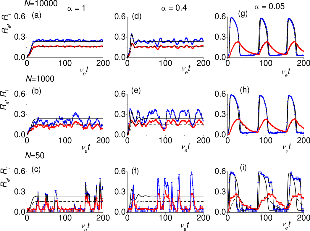
Figure 5: (color online). Fractions $R_{e}=\rho_{e}g_{e}$ and $R_{i}=\rho_{i}g_{i}$ of active excitatory and inhibitory neurons versus time. (a)-(c): $\alpha=1$ (region (I)). (d)-(f): $\alpha=0.4$ (region (II) ). (g)-(i): $\alpha=0.05$ (region (III)). Solid (dashed) lines show theoretical $R_{e}$ ($R_{i}$) from Eqs. (8). Blue (red) symbols refer to $R_{e}$ ($R_{i}$) from simulations at $N=10000$ (1st row), 1000 (2nd row), and 50 (third row). $F=0.05$, $g_{i}=0.4$, $c=20$, $\Omega=3$, $\mu_{2}=0$.

VI Simulations

Our simulations supported the theoretical results. Random networks with $N$ neurons were constructed by establishing directed links between any neuron $i$ and neuron $j$, with probability $c/N$. In the initial configuration all neurons were inactive. The state of each neuron is then updated every $\Delta t$ time units (parallel update) according to stochastic rules (i)-(iv). [Any other initial configuration may be also used.] The value of the time step $\Delta t$ was chosen such that the probabilities $f\Delta t$, $\mu_{1}\Delta t$, and $\mu_{2}\Delta t$ of the stochastic processes (i)-(iv) in Sec. II for excitatory and inhibitory neurons were sufficiently small. Reliable results were obtained when these probabilities were about 0.1 or smaller. Figure 5 represents typical numerical results obtained for systems of different sizes. All parameters used in simulations are presented in the caption to Fig. 5. For a given number of neurons $N$ we constructed several realizations of networks, and then we simulated their stochastic dynamics, using the rules (i)-(iv) in Sec. II. As one would expect, for the considered stochastic model, different runs and different realizations of neural networks differ slightly one from another. With increasing $N$ these differences become smaller and smaller, so these are standard run-to-run and realization-to-realization variations.

Figure 5 shows a full set of regimes. One can see that in regimes with exponential relaxation and decaying oscillations the irregular activity of neurons decreases with increasing $N$. Already at $N=1000$, a stimulation with $F>F_{c}$ activates a finite fraction of neurons in agreement with the theory, though there are strong irregular fluctuations around the steady state. In a small network of 50 neurons stochastic effects are strong and suppress the global activation. In Fig. 5 we also compare oscillations predicted by Eq. (8) to our simulations. Interestingly, these oscillations have a saw-tooth shape. Their period and shape depend on the parameters of the model such as $F$, $\alpha$, $c$, $\Omega$, and $g_{i}$. The theory and simulations are in very good agreement at $N=10000$. Actually we found good agreement with only $N=1000$. Surprisingly, the predicted oscillations emerge even in small groups of 50 neurons where strong stochastic effects and non negligible clustering could be expected. For $c=20$ and $N=50$ the mean clustering coefficient is $C=c/N=0.4$ ab02 ; dgm08 , which is close to the value $C=0.53$ found in the macaque visual cortex Sporns04 . This intrinsic property of small groups of neurons to oscillate may be very important for understanding communication between neuronal groups in the brain Fries05 .

VII Discussion

First let us discuss the assumptions and approximations which are the basis of our stochastic approach to noisy neural networks, and explain the biological meaning of the model parameters from the point of view of experimental and theoretical neuroscience.

In our model, activation of neurons by stimulus is a stochastic process with a characteristic time which is equal to the reciprocal rate $1/\mu_{1}$. In the brain, stochasticity in activation of neurons by stimulus may appear in trial-to-trial variability of the first-spike latency of neurons. The first-spike latency of a given neuron is defined as the time from the onset of a stimulus to the time of appearance of the first spike. The first-spike latency can depend on many parameters. For example, for auditory neurons it depends on the amplitude and frequency of stimulus heil04 . We suppose that the reciprocal rate $1/\mu_{1}$ is of the order of the mean first-spike latency of neurons. For simplicity, we assume that $1/\mu_{1}$ is constant and does not depend on the input. The first-spike latency may be of the order of the period of tonic spiking or much larger if the input is near the threshold. In the mammalian cortex the latency of regular spiking neurons for a superthreshold input can be in the tens of milliseconds. This gives $\mu_{1}\sim 10-400$ Hz.

In our approach it is assumed that each neuron may be active spontaneously, that is, it may discharge without experimenter-controlled stimulations. At the present time, the mechanisms and functional significance of spontaneous neural activity are not well understood and it is a topical problem in experimental and theoretical neuroscience Ermentrout08 ; Faisal08 ; AmitBrunel997 ; dc05 . The typical spontaneous background activity observed in the cortex is 1-5 spikes/s. Interactions between neurons play an important role in this activity AmitBrunel997 . Spontaneous activity in the brain may be mediated by intrinsic, intracellular, generated activity and circuit feedback mechanisms. Neural activity in one region of the brain may propagate to other regions, circulating in recurrent loops. For example, neurons in the thalamus and the cerebral cortex form recurrent loops steriade00 . The study of spontaneous activity in neocortical slices mao01 gives evidence that supports both mechanisms. For our model a mechanism of spontaneous activity is unimportant. One can assume that spontaneous activity takes place by the intrinsic mechanism. Alternatively one can consider the neural network as part of a large system from which neurons receive random inputs. In real neural networks only a fraction of neurons are spontaneously active mao01 . In the present paper we study the case in which all excitatory and inhibitory neurons may be spontaneously active. One can show that if only some fraction of neurons is spontaneously active, the dynamics of the neural networks would be qualitatively the same.

Furthermore, we considered the activation of neurons by an external stimulus as a stochastic process. Experimental work supports this assumption. For example, it was revealed that a moving whisker can have only a 15% chance of generating spikes in a neuron in the mouse somatosensory cortex bs02 . Unfortunately, much less is known about stochastic processes of spontaneous deactivation of neurons. In our model, the reciprocal rate $1/\mu_{2}$ is the characteristic time at which neurons stop firing due to irregular fluctuations on the input or due to random processes taking place inside the cells. Recently it was shown that spontaneous activity of single neurons may be driven by noise which can not only activate but can also inhibit spiking activity of neurons of both type 1 and type 2 gjt08 ; tgj09 ; tj09 .

The rates of the stochastic processes discussed above can be found from statistical analysis of activation and inactivation events in neural networks. They can also be measured by use of the patch-clamp technique: one can stimulate presynaptic excitatory and inhibitory neurons and then measure the probability of activation of a postsynaptic neuron through the distribution of first-spike timing times.

The proposed stochastic model is not restricted to regular spiking neurons. One can also analytically study noisy neural networks with neurons which generate random spike trains, for example, Poisson spike trains as found in recordings from neurons in vivo and in vitro Faisal08 . The proposed stochastic approach can also be generalized to study analytically neural networks with neurons having the type 1 and 2 dynamical behavior shown in Fig. 1 for the case when correlations between presynaptic neurons may be neglected. However these generalizations are out of the scope of the present paper.

We found that even a small group of neurons reveals intrinsic oscillations which are robust against strong stochastic fluctuations (see Fig. 5). It means that despite noise, neurons in a small group can synchronize their dynamics. We believe that this result opens interesting possibilities to study and model communication between different groups of neurons and the transmission of activity from one group of neurons to another. In the recent review Fries05 , “neuronal communication between neuronal groups through neuronal coherence” was considered as a mechanism for cognitive dynamics. On the basis of neurophysiological data, Fries suggested that coherently oscillating neuronal groups can interact effectively Fries05 . This idea is based on an assumption that activated neuronal groups have an intrinsic tendency to oscillate. Our model supports this assumption, showing that oscillations indeed are an intrinsic property and robust against noise. In our model one can model communication between neural populations or neural modules. Synchronization of neurons or groups or modules of neurons in the regime with oscillations can play an important role in this communication. Indeed, our preliminary simulation of interacting neural communities reveals complex patterns of neural activities. On the basis of our stochastic model one could study the computational role of network oscillations and how oscillations contribute to the representation of information sp06 .

Real neural networks have a scale-free degree distribution Sporns04 rather than a simple Poisson distribution. A preliminary study of neural networks with a scale-free degree distribution showed that these networks demonstrate dynamical properties qualitatively similar to properties of the networks studied above.

Let us discuss possible experiments to test the proposed model. First, it would be interesting to observe hysteresis and neural avalanches like those found in Sec. IV near the discontinuous phase transition. A similar discontinuous phase transition was revealed in activations of living neural networks by a stimulus in recent works Eckmann07 . Neural avalanches in these biological systems can be found by use of microelectrode arrays as described in bp03 ; Plenz07 . Second, the theory predicts that the emergence of global oscillations is a dynamical phase transition. A strong enhancement of the response of a neural network to a periodic stimulus in the range of frequencies of these oscillations manifests this transition. These oscillations can be driven by an external stimulus, neural pacemakers or noise. Though we demonstrated this behavior for ideal neurons, we believe that it is a universal critical phenomenon if a sufficiently large group of neurons is involved in these oscillations. It would be interesting to observe experimentally this enhancement which in fact is stochastic resonance. This enhancement may be found, for example, in experiments similar to the experiments carried out by Fries et al. frrd01 who observed that neurons of macaque monkeys activated by the attendant stimulus show increased gamma-frequency (35 - 90 Hz) oscillations. One can expect that a response of the neurons to periodic stimulus in the gamma-band frequency will be enhanced near critical attention above which gamma-frequency oscillations emerge.

VIII Conclusion

In conclusion, based on experiments and ideas of cellular automata we developed a model of noisy neural networks with excitatory and inhibitory neurons and a complex network architecture. We considered neurons which are either inactive or fire a regular train of spikes with a given frequency (neurons with type 2 dynamical behavior). In this model we took into account spontaneous neural activity, which plays the role of noise, the activation of neurons by a stimulus, neural pacemakers, and interactions between neurons. We derived rate equations describing the evolution of the global neuronal activity. These equations are exact for infinite uncorrelated complex networks with arbitrary degree distributions, though for brevity, we presented results only for classical random graphs. This model has a complex phase diagram with self-organized active neural states, hybrid phase transitions, hysteresis phenomena and a rich array of behavior including decaying and stable oscillations, stochastic resonance, and neural avalanches. We showed that global oscillations and stochastic resonance are intrinsic properties of this non-linear dynamical system. The oscillations emerge when noise, i.e., the spontaneous neural activity, reaches a threshold level while stochastic resonance is a precursor of global oscillations. We also found that the network structure is important. The larger the connectivity the broader is the region with global oscillations. Our simulations revealed that even small groups of 50-1000 neurons display oscillations similar to large networks.

Further development of the model can be done by taking into account the real structure of neural networks (clustering, degree-degree correlations, modular structure, and other structural properties), a dependence of firing rate on input, variability of synapses, evolution of network structure, for example, considering growing networks, or variable strength of synapses, and so on. Apart from the perspectives discussed above, one can also apply this stochastic model to study communication between different groups of neurons and the transmission of activity from one group or module of neurons to another, taking into account noise and complex network architecture.

- (1) D. J. Watts and S. H. Strogatz, Nature 393, 409(1998).
- (2) R. Albert and A.-L. Barabási, Rev. Mod. Phys. 74, 47 (2002); S. N. Dorogovtsev and J. F. F. Mendes, Adv. Phys. 51, 1079 (2002); M. E. J. Newman, SIAM Review 45, 167 (2003).
- (3) O. Sporns, D. R. Chialvo, M. Kaiser, and C. C. Hilgetag, Trends Cogn. Sci. 8, 418 (2004); E. Bullmore and O. Sporns, Nature Reviews: Neuroscience, 10, 191 (2009).
- (4) G. Buzsáki, C. Geisler, D. A. Henze, and X.-J. Wang, Trends Neurosci. 27, 186 (2004).
- (5) S. N. Dorogovtsev, A. V. Goltsev, and J. F. F. Mendes, Rev. Mod. Phys. 80, 1275 (2008).
- (6) S. Boccaletti, V. Latora, Y. Moreno, M. Chavez, D. U. Hwang, Phys. Rep. 424, 175 (2006).
- (7) A Arenas, A D az-Guilera, J Kurths, Y Moreno, C Zhou, Phys. Rep. 469, 93 (2008).
- (8) G. B. Ermentrout, R. F. Galan, and N. N. Urban, Trends Neurosci. 32, 428 (2008).
- (9) A. A. Faisal, L. P. J. Selen, and D.M. Wolpert, Nat. Neurosci. 9, 292 (2008).
- (10) F. Moss, L. M. Ward, and W. G. Sannita, Clin. Neurophysiol. 115, 267 (2004).
- (11) M. D. McDonnell and D. Abbott, PLoS Comput. Biol. 5, e1000348 (2009).
- (12) J.-P. Eckmann, O. Feinerman, L. Gruendlinger, E. Moses, J. Soriano, and T. Tlusty, Phys. Rep. 449, 54 (2007); I. Breskin, J. Soriano, E. Moses, and T. Tlusty, Phys. Rev. Lett. 97, 188102 (2006); J. Soriano, M . Rodr guez Mart nez, T. Tlusty, and E. Moses. Proc. Natl. Acad. Sci. USA 105, 13758 (2008).
- (13) A. L. Hodgkin, J. Physiol. 107, 165 (1948).
- (14) E. M. Izhikevich, IEEE Trans. Neural Netw., 15, 1063 (2004 ).
- (15) E. M. Izhikevich, Dynamical Systems in Neuroscience, (MIT Press, Cambridge MA, 2007)
- (16) T. Tateno, A. Harsh, and H. P. C. Robinson, J. Neurophysiol. 92, 2283 (2004).
- (17) A. Bogaard, J. Parent, M. Zochowski, and V. Booth, J. Neurosci. 29, 1677 (2009).
- (18) N. F. Rulkov, Phys. Rev. E 65, 041922 (2002).
- (19) N. F. Rulkov, I. Timofeev, and M. Bazhenov, J. Comput. Neurosci. 17, 203 (2004).
- (20) B. Lindner, J. Garcia-Ojalvo, A. Neiman, and L. Schimansky-Geier, Phys. Rep. 392, 321 (2004).
- (21) D. Randell, W. Burggren, and K. Frenh, Eckert Animal Physiology: Mechanisms and Addaptations. (W. H. Freeman, NY, 1997).
- (22) F. C. Hoppensteadt and E. M. Izhikevich, Weakly Connected Neural Netwoks, (Springer-Verlag, New York, 1997).
- (23) B. Kriener, T. Tetzlaff, A. Aertsen, M. Diesmann, and S. Rotter, Neural Computation 20, 2185, (2008).
- (24) D. J. Amit, Modeling Brain Function (Cambridge University Press, NY, 1989).
- (25) B. Derrida, E. Gardner, and A. Zippelius, Europhys. Lett. 4, 167 (1987).
- (26) C. van Vreeswijk and H. Sompolinsky, Neural Comput. 10, 1321 (1998).
- (27) G. Grinstein and R. Linsker, Proc. Natl. Acad. Sci. USA 102, 9948 (2005).
- (28) D. J. Amit and N. Brunel, Cerebral Cortex 7, 237 (1997).
- (29) R. Pastor-Satorras and A. Vespignani, Phys. Rev. Lett. 86, 3200 (2001); Phys. Rev. E 63, 066117 (2001).
- (30) M. Catanzaro, M. Boguñá, and R. Pastor-Satorras, Phys. Rev. E 71, 056104 (2005).
- (31) B. Ermentrout and T.-W. Ko, Phil. Trans. R. Soc. A 367, 1097 (2009).
- (32) H. R. Wilson and J. D. Cowan, Biophys. J. 12, 1 (1972).
- (33) H. R. Wilson and J. D. Cowan, Kibernetik 13, 55 (1973).
- (34) S. N. Dorogovtsev, A. V. Goltsev, and J. F. F. Mendes, Phys. Rev. Lett. 96, 040601 (2006); Phys. Rev. E 73, 056101 (2006).
- (35) J. Beggs and D. Plenz, J. Neurosci. 23, 11167 (2003).
- (36) D. Plenz and T. C. Thiagarajan, Trends Neurosci. 30, 101 (2007).
- (37) L. Gammaitoni, P. Hanggi, P. Jung, and F. Marchesoni, Rev. Mod. Phys. 70, 223 (1998).
- (38) P. Fries, Trends Cogn. Sci. 9, 474 (2005).
- (39) P. Heil, Curr. Opinion Neurobiol. 14, 461 (2004).
- (40) S. Dehaene and J.-P. Changeux, PLoS Biology 3, 0910 (2005).
- (41) M. Steriade, Neuroscience 101, 243 (2000).
- (42) B. Q. Mao, F. Hamzei-Sichani, D. Aronov, R. C. Froemke, and R. Yuste, Neuron 32, 883 (2001).
- (43) M. Brecht and B. Sakmann, J. Physiol. 543, 49 (2002).
- (44) B. S. Gutkin, J. Jost, and H. C. Tuckwell, EPL 81, 20005 (2008); Theory Biosci. 127, 135 (2008).
- (45) H. C. Tuckwell, J. Jost, and B. S. Gutkin, Phys. Rev. E 80, 031907 (2009).
- (46) H. C. Tuckwell and J. Jost, Physica A 388, 4115 (2009).
- (47) T. J. Sejnowski and O. Paulsen, J. Nerosci., 26, 1673 (2006).
- (48) P. Fries, J. H. Reynolds, A. E. Rorie, and R. Desimone, Science 291, 1560 (2001).