Clarifying Forecasts of Dark Energy Constraints from Baryon Acoustic Oscillations

Abstract

The measurement of baryon acoustic oscillations (BAO) from a galaxy redshift survey provides one of the most promising methods for probing dark energy. In this paper, we clarify the assumptions that go into the forecasts of dark energy constraints from BAO. We show that assuming a constant $nP_{0.2}/G^{2}(z)$ (where $P_{0.2}$ is the real space galaxy power spectrum at $k=0.2\,h/$Mpc and redshift $z$) gives a good approximation of the observed galaxy number density expected from a realistic flux-limited galaxy redshift survey. We find that assuming $nP_{0.2}/G^{2}(z)=10$ gives very similar dark energy constraints to assuming $nP_{0.2}=3$, but the latter corresponds to a galaxy number density larger by $\sim$ 70% at $z=2$. We show how the Figure-of-Merit (FoM) for constraining dark energy depends on the assumed galaxy number density, redshift accuracy, redshift range, survey area, and the systematic errors due to calibration and uncertainties in the theory of nonlinear evolution and galaxy biasing. We find that an additive systematic noise of up to $0.4-0.5$% per $\Delta z=0.1$ redshift slice does not lead to significant decrease in the BAO FoM.

I Introduction

It has been more than a decade since the discovery of the cosmic acceleration Riess et al. (1998); Perlmutter et al. (1999). Illuminating the nature of dark energy, the unknown cause of the observed cosmic acceleration, has become a prominent task for the astronomy and physics communities.

Dark energy could be an unknown energy component quintessence , or a modification of general relativity modifiedgrav . These two classes of models can be differentiated if both the cosmic expansion history and growth history of cosmic large scale structure are accurately and precisely measured DEvsMG . Current observational data are consistent with dark energy being a cosmological constant, but other explanations are still allowed (see, for example, Data (2009)). See Reviews (2009) for recent reviews on dark energy research.

One of the most promising methods for probing dark energy is to use the baryon acoustic oscillations (BAO) in the observed 3-D galaxy distribution as a cosmological standard ruler BG03 ; SE03 ; BAO . At the last scattering of cosmic microwave background (CMB) photons, the acoustic oscillations in the photon-baryon fluid became frozen, and imprinted their signatures on both the CMB (the acoustic peaks in the CMB angular power spectrum) and the matter distribution (the BAO in the galaxy power spectrum). Because baryons comprise only a small fraction of matter, and the matter power spectrum has evolved significantly since last scattering of photons, BAO are much smaller in amplitude than the CMB acoustic peaks, and are washed out on small scales. BAO in the observed galaxy power spectrum have the characteristic scale determined by the comoving sound horizon at recombination, which is precisely measured by the CMB anisotropy data Spergel et al. (2007). In principle, the BAO scale can be extracted from data both in the transverse direction ($s_{\perp}$), and along the line-of-sight ($s_{\parallel}$). Comparing the observed BAO scales with the expected values gives the angular diameter distance $D_{A}(z)=r(z)/(1+z)$ (where $r(z)$ is the comoving distance) in the transverse direction, and the Hubble parameter $H(z)$ in the radial direction:

$$s_{\perp} \propto \frac{s}{D_{A}(z)}$$

$$s_{\parallel} \propto sH(z).$$ (1)

Seo & Eisenstein (2007) SE07 (henceforth SE07) provided simple fitting formulae for forecasting the accuracies of $s/D_{A}(z)$ and $s\,H(z)$ from future galaxy redshift surveys. In this paper, we will clarify the assumptions made in BAO forecasts, and investigate their implications. We will discuss the method in Sec.2, present results on BAO forecasts in Sec.3, and summarize in Sec.4.

II The method

The simplest and most widely used method to forecast constraints from future observations is to use the Fisher matrix formalism. The Fisher information matrix of a given set of parameters, ${\bf s}$, approximately quantifies the amount of information on ${\bf s}$ that we expect to get from our future data. The Fisher matrix can be written as

$$F_{ij}=-\frac{\partial^{2}\ln\,L}{\partial s_{i}\partial s_{j}},$$ (2)

where $L$ is the likelihood function, the expected probability distribution of the observables given parameters ${\bf s}$. The Cramér-Rao inequality states that no unbiased method can measure the $i$-th parameter with standard deviation less than $1/\sqrt{F_{ii}}$ if other parameters are known, and less than $\sqrt{({\bf F}^{-1})_{ii}}\,$ if other parameters are estimated from the data as well Kendall & Stuart (1969).

In the limit where the length scale corresponding to the survey volume is much larger than the scale of any features in the galaxy power spectrum $P_{g}(k)$, we can assume that the likelihood function for the band powers of a galaxy redshift survey is Gaussian Feldman94 . Then the Fisher matrix for estimating parameters from a galaxy redshift survey can be approximated as (Tegmark97, )

$$F_{ij}=\int_{k_{min}}^{k_{max}}\frac{\partial\ln P_{g}(\mbox{\bf k})}{\partial p_{i}}\frac{\partial\ln P_{g}(\mbox{\bf k})}{\partial p_{j}}\,V_{eff}(\mbox{\bf k})\,\frac{d\mbox{\bf k}^{3}}{2\,(2\pi)^{3}}$$ (3)

where $p_{i}$ are the parameters to be estimated from data, and the derivatives are evaluated at parameter values of the fiducial model. The effective volume of the survey

$$V_{eff}(k,\mu) = \int\mbox{d}^{3}\mbox{\bf r}\left[\frac{n(\mbox{\bf r})P_{g}(k,\mu)}{n(\mbox{\bf r})P_{g}(k,\mu)+1}\right]^{2}$$ (4)

$$= \left[\frac{nP_{g}(k,\mu)}{nP_{g}(k,\mu)+1}\right]^{2}V_{survey},$$

where the comoving number density $n$ is assumed to only depend on the redshift for simplicity; $\mu=\mbox{\bf k}\cdot\hat{\mbox{\bf r}}/k$, with $\hat{\mbox{\bf r}}$ denoting the unit vector along the line of sight; k is the wavevector with $|\mbox{\bf k}|=k$. Note that the Fisher matrix $F_{ij}$ is the inverse of the covariance matrix of the parameters $p_{i}$ if the $p_{i}$ are Gaussian distributed. Eq.(3) propagates the measurement errors in $\ln P_{g}(\mbox{\bf k})$ (which are proportional to $[V_{eff}(\mbox{\bf k})]^{-1/2}$) into measurement errors for the parameters $p_{i}$. Note that Eq.(3) can be rewritten as

$$F_{ij} = V_{survey}\int_{-1}^{1}d\mu\int_{k_{min}}^{k_{max}}\frac{\partial P_{g}(k,\mu)}{\partial p_{i}}\frac{\partial P_{g}(k,\mu)}{\partial p_{j}}\,\cdot$$ (5)

$$\cdot\left[\frac{1}{P_{g}(k,\mu)+n^{-1}}\right]^{2}\frac{2\pi k^{2}dk}{2\,(2\pi)^{3}},$$

where $\mu=\hat{\mbox{\bf k}}\cdot\hat{\mbox{\bf r}}$.

II.1 The “wiggles only” fitting formulae

SE07 SE07 provided simple fitting formulae for forecasting the accuracies of $s/D_{A}(z)$ and $s\,H(z)$ from future galaxy redshift surveys. Essentially, they approximated Eq.(5) with

$$F_{ij} \simeq V_{survey}\int_{-1}^{1}d\mu\int_{k_{min}}^{k_{max}}\frac{\partial P_{b}(k,\mu|z)}{\partial p_{i}}\frac{\partial P_{b}(k,\mu|z)}{\partial p_{j}}\,\cdot$$ (6)

$$\cdot\left[\frac{1}{P_{g}^{lin}(k,\mu|z)+n^{-1}}\right]^{2}\frac{2\pi k^{2}dk}{2\,(2\pi)^{3}},$$

where $P_{b}(k,\mu|z)$ is the power spectrum that contains baryonic features. The linear galaxy power spectrum

$$P_{g}^{lin}(k,\mu|z) = P_{g,r}^{lin}(k|z)\,R(\mu)$$ (7)

$$P_{g,r}^{lin}(k|z) = b(z)^{2}\left[\frac{G(z)}{G(0)}\right]^{2}\,P_{m}^{lin}(k|z=0)$$ (8)

where $P_{g,r}^{lin}(k|z)$ is the linear galaxy power spectrum in real space, $b$ is the bias factor, $G(z)$ is the growth factor, and $P_{m}^{lin}(k|z=0)$ is the present day linear matter power spectrum. $R(\mu)$ is the linear redshift distortion factor given by

$$R(\mu)=\left(1+\beta\mu^{2}\right)^{2}.$$ (9)

The power spectrum that contains baryonic features, $P_{b}(k,\mu)$, is given by

$$P_{b}(k,\mu|z) = \sqrt{8\pi^{2}}A_{0}\,P_{g}^{lin}(k_{0.2},\mu|z)\frac{\sin(x)}{x}\cdot$$ (10)

$$\cdot\exp\left[-(k\Sigma_{s})^{1.4}-\frac{k^{2}\Sigma_{nl}^{2}}{2}\right],$$

where we have define

$$k_{0.2} \equiv 0.2\,h\,{\rm Mpc}^{-1}$$ (11)

$$x \equiv \left(k^{2}_{\perp}s^{2}_{\perp}+k^{2}_{\parallel}s^{2}_{\parallel}\right)^{1/2}$$ (12)

$$k_{\parallel} = \mbox{\bf k}\cdot\hat{\mbox{\bf r}}=k\mu$$ (13)

$$k_{\perp} = \sqrt{k^{2}-k^{2}_{\parallel}}=k\sqrt{1-\mu^{2}}.$$ (14)

The nonlinear damping scale

$$\Sigma_{nl}^{2} = (1-\mu^{2})\Sigma_{\perp}^{2}+\mu^{2}\Sigma^{2}_{\parallel}$$

$$\Sigma_{\parallel} = \Sigma_{\perp}(1+f_{g})$$

$$\Sigma_{\perp} = 12.4\,h^{-1}{\rm Mpc}\,\left(\frac{\sigma_{8}}{0.9}\right)\cdot 0.758\,\frac{G(z)}{G(0)}\,p_{NL}$$ (15)

$$= 8.355\,h^{-1}{\rm Mpc}\,\left(\frac{\sigma_{8}}{0.8}\right)\cdot\frac{G(z)}{G(0)}\,p_{NL},$$

where $f_{g}=d\ln G(z)/d\ln a$ denotes the growth rate of matter density fluctuations. The parameter $p_{NL}$ indicates the remaining level of nonlinearity in the data; with $p_{NL}=0.5$ (50% nonlinearity) as the best case, and $p_{NL}=1$ (100% nonlinearity) as the worst case SE07 . For a fiducial model based on WMAP3 results Spergel et al. (2007) ($\Omega_{m}=0.24$, $h=0.73$, $\Omega_{\Lambda}=0.76$, $\Omega_{k}=0$, $\Omega_{b}h^{2}=0.0223$, $\tau=0.09$, $n_{s}=0.95$, $T/S=0$), $A_{0}=0.5817$, $P_{0.2}=2710\,\sigma_{8,g}^{2}$, the Silk damping scale $\Sigma_{s}=8.38\,h^{-1}{\rm Mpc}$.

Defining

$$p_{1} = \ln s_{\perp}^{-1}=\ln(D_{A}/s),$$ (16)

$$p_{2} = \ln s_{\parallel}=\ln(sH),$$ (17)

substituting Eq.(10) into Eq.(6), and making the approximation of $\cos^{2}x\sim 1/2$, we find

$$F_{ij}\simeq V_{survey}A_{0}^{2}\int_{0}^{1}\mbox{d}\mu\,f_{i}(\mu)\,f_{j}(\mu)\int_{0}^{k_{max}}\mbox{d}k\,k^{2}\cdot$$

$$\hskip 1.4457pt\cdot\left[\frac{P^{lin}_{m}(k|z=0)}{P^{lin}_{m}(k_{0.2}|z=0)}+\frac{1}{nP^{lin}_{g}(k_{0.2},\mu|z)\,e^{-k^{2}\mu^{2}\sigma_{r}^{2}}}\right]^{-2}$$

$$\hskip 1.4457pt\cdot\exp\left[-2(k\Sigma_{s})^{1.4}-k^{2}\Sigma_{nl}^{2}\right],$$ (18)

where $P_{g}^{lin}(k_{0.2},\mu|z)$ is given by Eq.(7) with $k=k_{0.2}$. Note that we have added the damping factor, $e^{-k^{2}\mu^{2}\sigma_{r}^{2}}$, due to redshift uncertainties, with

$$\sigma_{r}=\frac{\partial r}{\partial z}\,\sigma_{z}$$ (19)

where $r$ is the comoving distance. For a flat universe, $r=\int_{0}^{z}dz^{\prime}/H(z^{\prime})$. The functions $f_{i}(\mu)$ are given by

$$f_{1}(\mu) = \partial\ln x/\partial\ln p_{1}=\mu^{2}-1$$ (20)

$$f_{2}(\mu) = \partial\ln x/\partial\ln p_{2}=\mu^{2}.$$ (21)

II.2 Full power spectrum calculation

In order to compare the “wiggles only” method and the full power spectrum method for BAO forecast, we must include the nonlinear effects in the same way in both methods. In the full power spectrum method, the observed power spectrum is reconstructed using a particular reference cosmology, including the effects of bias and redshift-space distortions SE03 :

$$P_{obs}(k^{ref}_{\perp},k^{ref}_{\parallel}) = \frac{\left[D_{A}(z)^{ref}\right]^{2}H(z)}{\left[D_{A}(z)\right]^{2}H(z)^{ref}}\,b^{2}\left(1+\beta\,\mu^{2}\right)^{2}\cdot$$ (22)

$$\hskip-21.68121pt\cdot\left[\frac{G(z)}{G(0)}\right]^{2}P_{matter}(k|z=0)+P_{shot},$$

where

$$k^{ref}_{\perp}=k_{\perp}\,\frac{D_{A}(z)}{D_{A}(z)^{ref}},\hskip 14.22636ptk^{ref}_{\parallel}=k_{\parallel}\,\frac{H(z)^{ref}}{H(z)},$$ (23)

and $\mu^{2}=k^{2}_{\parallel}/k^{2}=k^{2}_{\parallel}/(k^{2}_{\perp}+k^{2}_{\parallel})$. The values in the reference cosmology are denoted by the subscript “ref”, while those in the true cosmology have no subscript.

Following Seo & Eisenstein (2007) SE07 , we include nonlinear effects in the full power spectrum calculation by modifying the derivatives of $P(\mbox{\bf k})$ with respect to the parameters $p_{i}$, i.e.,

$$\frac{\partial P_{g}(k,\mu|z)}{\partial p_{i}}=\frac{\partial P_{g}^{lin}(k,\mu|z)}{\partial p_{i}}\cdot\exp\left(-k^{2}\Sigma_{nl}^{2}/2\right).$$ (24)

Eq.(5) becomes

$$F_{ij} = V_{survey}\int_{-1}^{1}d\mu\int_{k_{min}}^{k_{max}}\frac{\partial\ln P_{g}^{lin}(k,\mu)}{\partial p_{i}}\frac{\partial\ln P_{g}^{lin}(k,\mu)}{\partial p_{j}}\,\cdot$$ (25)

$$\cdot\left[\frac{nP_{g}^{lin}(k,\mu)}{nP_{g}^{lin}(k,\mu)+1}\right]^{2}\,e^{-k^{2}\Sigma_{nl}^{2}}\frac{2\pi k^{2}dk}{2\,(2\pi)^{3}}.$$

II.3 Figure of merit and dark energy parameters

The DETF defined the dark energy figure of merit (FoM) to be the inverse of the area enclosed by the 95% confidence contour for the parameters ($w_{0},w_{a}$), assuming a dark energy equation of state $w_{X}(z)=w_{0}+(1-a)w_{a}$ Chev01 (2001). It is most convenient to define a relative generalized FoM Wang (2008)

$${\rm FoM}_{r}=\frac{1}{\sqrt{{\rm det}\,{\rm Cov}(f_{1},f_{2},f_{3},...)}},$$ (26)

where $\{f_{i}\}$ are the chosen set of dark energy parameters. This definition has the advantage of being easy to calculate for either real or simulated data. When applied to ($w_{0},w_{a}$), we find

$${\rm FoM}_{r}=\frac{1}{\sqrt{{\rm det}\,{\rm Cov}(w_{0},w_{a})}}=\frac{1}{\sqrt{\sigma^{2}_{w_{0}}\sigma^{2}_{w_{a}}-\sigma^{2}_{w_{0},w_{a}}}},$$ (27)

which differs by a factor of 6.17$\pi$ from the DETF definition. This is the FoM that has been widely used, and tabulated in the DETF report.

The most sensible FoM requires choice of dark energy parameters that are least correlated Wang (2008). A good choice is to use ($w_{0},w_{0.5}$) from

$$w_{X}(a)=3w_{0.5}-2w_{0}+3\left(w_{0}-w_{0.5}\right)\,a$$ (28)

$$X(z)=(1+z)^{3(1-2w_{0}+3w_{0.5})}\exp\left[9(w_{0}-w_{0.5})\,\frac{z}{1+z}\right],$$

where $w_{0.5}$ is the value of $w_{X}$ at $z=0.5$. The correlation of $(w_{0},w_{0.5})$ is much smaller than that of $(w_{0},w_{a})$. For real data analyzed using Marcov Chain Monte Carlo (MCMC), the covariance matrix of $(w_{0},w_{0.5})$ and $(w_{0},w_{a})$ cannot be transformed, since choosing $(w_{0},w_{0.5})$ and choosing $(w_{0},w_{a})$ as the base parameters correspond to different priors, if uniform priors are assumed for the base parameters. For Fisher matrix forecast, one can simply transform the covariance matrix of $(w_{0},w_{a})$ into that of $(w_{0},w_{0.5})$ by using

$$w_{0.5}=w_{0}+w_{a}/3.$$ (29)

II.4 Choice of redshift bins

There has been some confusion in the literature about the optimal choice of redshift bins in constraining dark energy. This choice should depend on the observational method considered. For a galaxy redshift survey, the observables are $s/D_{A}$ and $sH$ (length scales extracted from data analysis). Since these scales are assumed to be constant in each redshift slice, the redshift slices should be chosen such that the variation of $1/D_{A}(z)$ and $H(z)$ in each redshift slice remain roughly constant with $z$.

For a flat universe, the variations of $H(z)$ and $1/D_{A}(z)$ with $z$ are

$$\frac{d(H/H_{0})}{dz} = \frac{3\Omega_{m}(1+z)^{2}+\Omega_{X}X^{\prime}(z)}{2E(z)}$$ (30)

$$\frac{d(1/D_{A})}{dz} = \frac{1}{r(z)}\left[1-\frac{1+z}{H(z)\,r(z)}\right]$$ (31)

$$E^{2}(z) = \frac{H^{2}(z)}{H_{0}^{2}}=\Omega_{m}(1+z)^{3}+\Omega_{X}X(z),$$ (32)

where $X(z)\equiv\rho_{X}(z)/\rho_{X}(0)$ is the dark energy density function. $X(z)=1$ for a cosmological constant. Fig.1 shows the variations of $H(z)$ and $1/D_{A}(z)$ with $z$ for a fiducial flat $\Lambda$CDM model. The amplitude of variation in $H(z)$ increases slowly with $z$. The amplitude of variation in $1/D_{A}(z)$ decreases with $z$, and stablize for $z\mathrel{\mathchoice{\lower 3.6pt\vbox{\halign{$\mathsurround=0pt\displaystyle\hfill#\hfil$\cr>\crcr\sim\crcr}}}{\lower 3.6pt\vbox{\halign{$\mathsurround=0pt\textstyle\hfill#\hfil$\cr>\crcr\sim\crcr}}}{\lower 3.6pt\vbox{\halign{$\mathsurround=0pt\scriptstyle\hfill#\hfil$\cr>\crcr\sim\crcr}}}{\lower 3.6pt\vbox{\halign{$\mathsurround=0pt\scriptscriptstyle\hfill#\hfil$\cr>\crcr\sim\crcr}}}}1$. Thus choosing a constant $\Delta z$ for redshift slices is the optimal choice. Choosing constant $\Delta z$ avoids significantly degrading the approximation of $H(z)$ being constant in each redshift slice as $z$ increases, while the approximation of $D_{A}(z)$ being constant becomes increasingly better as $z$ increases. This makes sense since $H(z)$ measurements carry more weight in constraining dark energy than the $D_{A}(z)$ measurements.

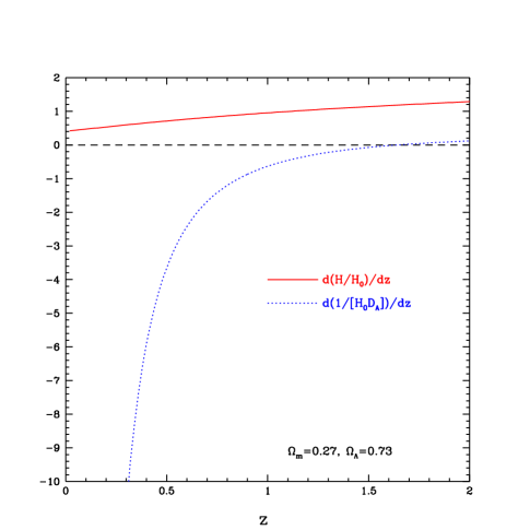
Figure 1: The variations of $H(z)$ and $1/D_{A}(z)$ with $z$.

III Results

We find that the fitting formulae, Eq.(18), give errors of $\ln(s/D_{A})$ and $\ln(sH)$ that match those from the full Fisher matrix, Eq.(25), to better than $\sim$ 10-20%. We have applied the fitting formulae, Eq.(18), to investigate the dependence of the forecast of dark energy constraints from BAO on various survey parameters. We adopt the Dark Energy Task Force (DETF) fiducial model, with $\Omega_{m}h^{2}=0.146$, $\Omega_{b}h^{2}=0.024$, $h=0.725$, $\Omega_{k}=0$ $w=-1$, and $n_{s}=1.0$ deft (2006). We assume $\sigma_{8,m}(z=0)=0.8$ Komatsu08 , and $\sigma_{8,g}(z=0)=1$. We compute the matter transfer function using CMBFAST 4.5.1 CMBFAST . Table 1 lists the parameter values in the DETF model and the “other” model for comparison (all are present day values). We take $k_{min}=10^{-4}h\,$Mpc^-1, and $k_{max}=0.5\,h\,$Mpc^-1 SE07 .

Table 1: Two fiducial cosmological models

name	$\Omega_{m}$	$\Omega_{\Lambda}$	$h$	${\Omega_{b}}h^{2}$	$\tau$	$n_{s}$	$\sigma_{8,m}$	$\sigma_{8,g}$
DETF	.2778	.7222	.725	.024	.05	1	.8	1
other	.24	.76	.73	.0223	.09	.95	.761	1

III.1 Dependence on galaxy number density

For a given BAO survey, the galaxy number density $n(z)$ and bias function $b(z)$ should be modeled using available data and supplemented by cosmological N-body simulations that include galaxies Angulo08 . Since $n(z)$ and $b(z)$ depend on survey parameters such as the flux limit and the target selection method, a more generic galaxy number density given by assuming $nP_{0.2}\equiv nP_{g}^{r}(k_{0.2}|z)=\,$constant is often used in BAO forecasts, where $P_{g}^{r}(k_{0.2}|z)$ is the real space power spectrum of galaxies at $k=0.2\,h\,$Mpc^-1 and redshift $z$. Fig.2 shows the number of galaxies per $\Delta z=0.1$ slice per unit volume and per (deg)² respectively, multiplied by $b^{2}(z)$. Clearly, assuming a constant $nP_{0.2}$ corresponds to assuming that $n(z)b^{2}(z)$ increases faster than a linear function in $z$, most likely faster than the increase in the galaxy bias function $b(z)$ Sumi09 ; Orsi09 , thus implying an assumed galaxy number density $n(z)$ that increases with redshift.

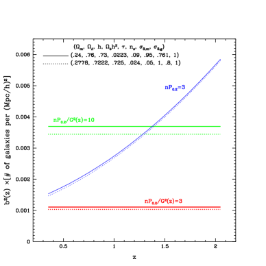
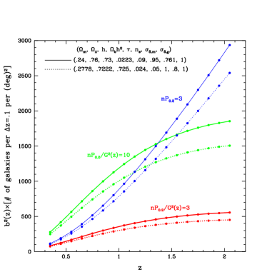
Figure 2: The comoving number density of galaxies per unit comoving volume (upper panel) and per (deg)² (lower panel). The results for two different fiducial cosmological models are shown, the “other” model (solid), and the DETF model (dotted).

A typical flux-limited galaxy redshift survey has a galaxy number density distribution that peaks at some intermediate redshift (as the volume per redshift slice increases with $z$), and decreases toward the high $z$ end of the survey (as the increase in the number of galaxies fainter than the flux limit dominates over the increase in volume per redshift slice). For a galaxy redshift survey with limited resources, photometric pre-selection could be used to alter $n(z)$ to cut out low redshift galaxies, and validate the assumption of constant $nP_{0.2}$. However, this would correspond to $nP_{0.2}<1$. It is challenging to achieve $nP_{0.2}>1$ at $z=2$ even for the most optimistic space-based galaxy redshift survey SPACE (2007); Geach09 . Thus it is misleading to use $nP_{0.2}=3$ to forecast the dark energy constraints from a space-based survey.

We propose the following alternative assumption about the observed galaxy number density:

$$nP_{0.2}/G^{2}(z)=n\,b^{2}(z)P_{m}(k_{0.2}|z=0)=\mbox{constant}.$$ (33)

Fig.3 shows the expected $nP_{0.2}$ assuming constant $nP_{0.2}/G^{2}(z)$ in the DETF model. Assuming a constant $nP_{0.2}/G^{2}(z)$ allows us to avoid assuming an unrealistically high $nP_{0.2}$ at the high redshift end, while at the same time retain the increasingly higher $nP_{0.2}$ easily achievable at intermediate and lower redshifts that play a key role in tightening the dark energy constraints.

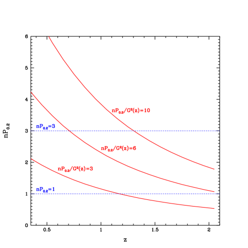
Figure 3: The expected $nP_{0.2}$ assuming constant $nP_{0.2}/G^{2}(z)$ in the DETF model.

In forecasting dark energy FoM from BAO, it is important to specify whether a constant $nP_{0.2}$ or constant $nP_{0.2}/G^{2}(z)$ is assumed. Fig.4 shows the fractional errors of $(sH)$ and $(s/D_{A})$ per $\Delta z=0.1$ slice expected from a 28,000 (deg)² galaxy redshift survey with $\sigma_{z}/(1+z)=0.001$, using the “wiggles only” fitting formulae of Eq.(18), for different assumptions about the observed galaxy number density. Note that for the “other” model, our results are in excellent agreement with the results of SE07 SE07 for $nP_{0.2}=3$ (thin lines with squares, compare with the dashed lines in Fig.3 of SE07), and for the cosmic variance case, i.e., zero shot noise and zero nonlinearity (thin lines with triangles, compare with the solid lines in Fig.3 of SE07).

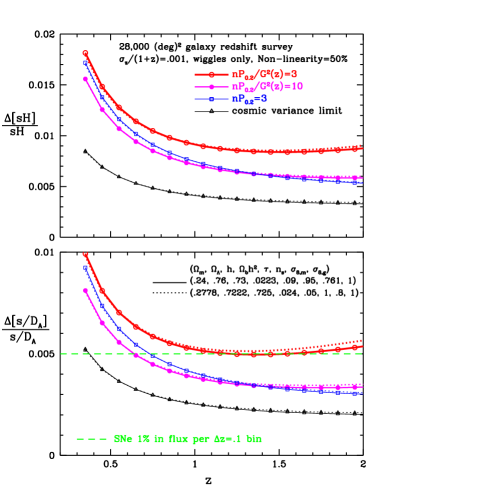
Figure 4: The fractional errors of $(sH)$ and $(s/D_{A})$ per $\Delta z=0.1$ slice expected from a 28,000 (deg)² galaxy redshift survey with $\sigma_{z}/(1+z)=0.001$, using our “wiggles only” modified formula of Eq.(18), for different assumptions about the observed galaxy number density The results for two different fiducial cosmological models are shown, the “other” model (solid), and the DETF model (dotted).

Fig.5 shows the 68.3% joint confidence contours for ($w_{0},w_{a}$) and ($w_{0},w_{0.5}$) (see Sec.II.3 for the definition of the parameters) for the three different galaxy number densities shown in Fig.2 and Fig.4. The DETF fiducial model is assumed. It is interesting to note that assuming $nP_{0.2}/G^{2}(z)=10$ gives very similar dark energy constraints to assuming $nP_{0.2}=3$, but the latter corresponds to a galaxy number density larger by $\sim$ 70% at $z=2$ (see Fig.3).

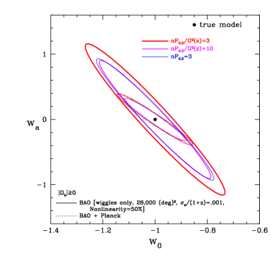
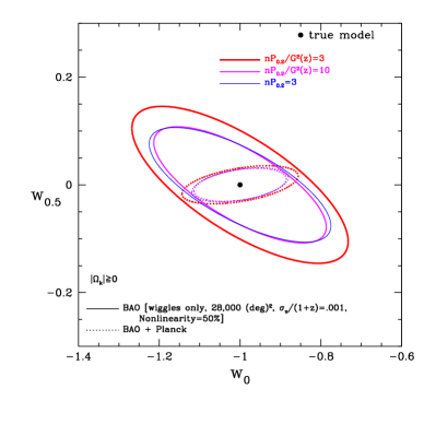
Figure 5: The 68.3% joint confidence contours for ($w_{0},w_{a}$) and ($w_{0},w_{0.5}$) for the three different galaxy number densities shown in Fig.2 and Fig.4. The DETF fiducial model is assumed.

Fig.6 shows the relative dark energy FoM, FoM_r (defined in Sec.II.3), for a galaxy redshift survey covering 28,000 (deg)² and $0.3<z<2.1$, as a function of galaxy number density. The dashed lines in Fig.6 show the results of using the full $P(k)$ method (see Eq.[25]). The full $P(k)$ method boosts the FoM by a factor of $\sim$3-4, with more gain for higher galaxy number densities.

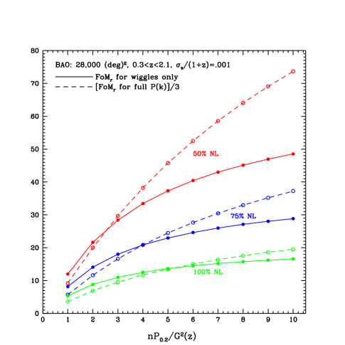
Figure 6: The relative dark energy FoM, FoM_r, for a galaxy redshift survey covering 28,000 (deg)² and $0.3<z<2.1$, as a function of galaxy number density. Both BAO wiggles only method (solid lines) and the full $P(k)$ method (dashed lines) are shown. The DETF fiducial model is assumed.

III.2 Dependence on other survey parameters

We now study the dependence of the dark energy FoM on the other survey parameters, redshift accuracy, redshift range, and survey area. We show all our results for two representative galaxy number densities, $nP_{0.2}/G^{2}(z)=3$ and 10.

Fig.7 shows the FoM_r for a galaxy redshift survey covering 28,000 (deg)² and $0.3<z<2.1$, as a function of the redshift accuracy. The FoM decreases quickly as $\sigma_{z}/(1+z)$ increases beyond 0.001. Increasing the redshift accuracy to $\sigma_{z}/(1+z)<0.001$ does not have a significant impact.

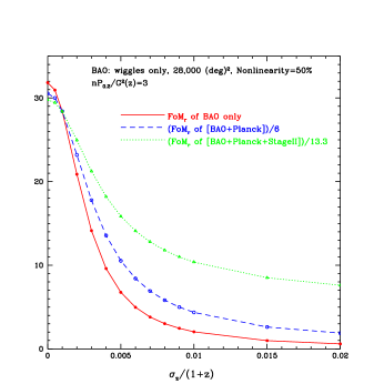
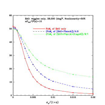
Figure 7: The relative dark energy FoM, FoM_r, for BAO wiggles only from a galaxy redshift survey covering 28,000 (deg)² and $0.3<z<2.1$, as a function of the redshift accuracy. The DETF fiducial model is assumed.

Fig.8 shows FoM_r for a galaxy redshift survey covering 28,000 (deg)² and $\sigma_{z}/(1+z)=.001$, as a function of $z_{max}$ for $z_{min}=0.5$ (upper panel), and as a function of $z_{min}$ for $z_{max}=2$ (lower panel). Decreasing $z_{max}$ and increasing $z_{min}$ both significantly decrease the FoM for BAO only.

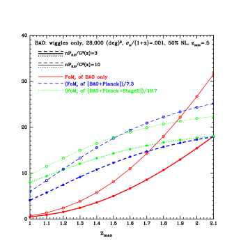
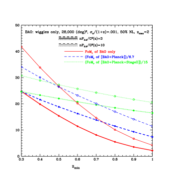
Figure 8: The relative dark energy FoM, FoM_r, for BAO wiggles only from a galaxy redshift survey covering 28,000 (deg)² and $\sigma_{z}/(1+z)=.001$, as a function of $z_{max}$ for $z_{min}=0.5$ (upper panel), and as a function of $z_{min}$ for $z_{max}=2$ (lower panel). The DETF fiducial model is assumed.

Fig.9 shows the FoM for a galaxy redshift survey covering $0.3<z<2.1$ with $\sigma_{z}/(1+z)=.001$, as a function of survey area. The BAO only constraints scale linearly with survey area. This is as expected, since no priors are added, and the constraints on dark energy parameters scale with $1/\sqrt{\mbox{area}}$. The more external priors are added, the more slowly the FoM increases with survey area. Thus the FoM of (BAO+Planck) increases more slowly with area than that of BAO only, and the FoM of (BAO+Planck+StageII) increases with area even more slowly.

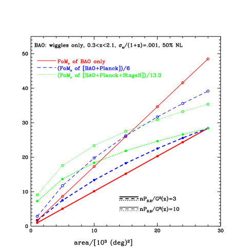
Figure 9: The relative dark energy FoM, FoM_r, for BAO wiggles only from a galaxy redshift survey covering $0.3<z<2.1$ with $\sigma_{z}/(1+z)=.001$, as a function of survey area. The DETF fiducial model is assumed.

III.3 Dependence on systematic uncertainties

There are two types of systematic uncertainties for BAO. One type of uncertainty is due to the calibration of the sound horizon by CMB data. The other type of uncertainty is due to the intrinsic limitations of the BAO method, for example, the uncertainties in the theory of nonlinear evolution and galaxy biasing Angulo08 .

WMAP five year observations gives $\Delta s/s\sim 1.3$% Komatsu08 . We expect that Planck will give $\Delta s/s\sim 0.2$% planck (2007). Note that $s$ appears as an overall scale parameter in the observables $(s/D_{A})$ and $(sH)$, and is assumed to be statistically independent from $(s/D_{A})$ and $(sH)$. Thus the uncertainty in $s$ has no effect on the dark energy FoM for the BAO wiggles only method. However, when other data are combined with the BAO (wiggles only) data, the overall dark energy FoM is decreased due to the uncertainty in $s$. If the parameter set used is $(w_{0},w_{a},\Omega_{X},\Omega_{k},\Omega_{m}h^{2})$ for the BAO dark energy covariance matrix, then $\Delta s\neq 0$ only modifies the diagonal matrix for $\Omega_{m}h^{2}$ by adding a term

$$\Delta C_{DE,55}^{BAO}=\left(2\Omega_{m}h^{2}\right)^{2}\left(\Delta s/s\right)^{2}.$$ (34)

The Planck prior of $\Delta s/s\sim 0.2$% has a very small effect on the FoM.

Our current modeling of intrinsic BAO systematic effects are at the $\sim$1-2% level for realistic N-body simulations that include galaxies (not just dark matter or dark matter haloes) Angulo08 . Correcting the bias in the estimated BAO scale due to systematic effects will likely lead to an increase in the uncertainty of the derived BAO scale Sanchez08 . In order to make realistic assessment of dark energy constraints from BAO, one should allow for some level of remaining system uncertainty in each redshift bin.

We show the effect of systematic uncertainty in two different ways. First, we show the effect of nonlinear effects explicitly, using the parametrization shown in Eq.(II.1), with $p_{NL}$ indicating the level of remaining nonlinearity. Secondly, we will show the effect of additive systematic noise in each redshift slice due to the incomplete removal or imperfect modeling of nonlinear effects or scale-dependent bias.

Fig.6 shows the relative dark energy FoM for three levels of nonlinearity: 50%, 75%, and 100%. Clearly, dark energy constraints from BAO are extremely sensitive to the level of nonlinearity assumed. Fig.10 shows the FoM_r as a function of the level of nonlinearity for two representative galaxy number distributions.

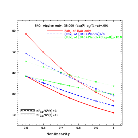
Figure 10: The relative dark energy FoM, FoM_r, for BAO wiggles only from a galaxy redshift survey covering 28,000 (deg)² and $0.3<z<2.1$, as a function of the level of nonlinearity. The DETF fiducial model is assumed.

Fig.11 shows the FoM_r, for a galaxy redshift survey covering 28,000 (deg)² and $0.3<z<2.1$, as a function of the level of additive systematic errors in each redshift bin. The pessimistic case considered by the DETF, $\sigma_{sys}^{i}=0.01\times\sqrt{5/\Delta z_{i}}$ gives 0.0224 for $\Delta z=0.1$, beyond the range of Fig.11. An additive systematic error of 0.5% per $\Delta z=0.1$ redshift slice would decrease the BAO FoM by 23% for $nP_{0.2}/G^{2}(z)=3$, and 34.5% for $nP_{0.2}/G^{2}(z)=10$. Note however, the larger galaxy number density should allow better modeling of the systematic effects, thus the systematic errors should be lower for $nP_{0.2}/G^{2}(z)=10$. An additive systematic error of 0.35% per $\Delta z=0.1$ redshift slice would decrease the BAO FoM by 21% for $nP_{0.2}/G^{2}(z)=10$.

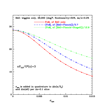
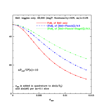
Figure 11: The relative dark energy FoM, FoM_r, for BAO wiggles only from a galaxy redshift survey covering 28,000 (deg)² and $0.3<z<2.1$, as a function of the level of systematic errors in each redshift bin. The DETF fiducial model is assumed.

IV Summary

We have studied the various assumptions that go into the BAO forecasts, using the fitting formulae for BAO (“wiggles only”) SE07 . We have shown that assuming $nP_{0.2}/G^{2}(z)=\,$constant gives a more realistic approximation of the observed galaxy number density than $nP_{0.2}=\,$constant. We find that assuming $nP_{0.2}/G^{2}(z)=10$ gives very similar dark energy constraints to assuming $nP_{0.2}=3$, but the latter corresponds to a galaxy number density larger by $\sim$ 70% at $z=2$ (see Fig.3).

Assuming that $nP_{0.2}/G^{2}(z)=\,$constant, we have shown how the FoM for constraining dark energy depends on the assumed galaxy number density, redshift accuracy, redshift range, survey area, and the systematic errors due to uncertainties in the theory of nonlinear evolution and galaxy biasing.

We find that $\sigma_{z}/(1+z)=0.001$ is an optimal redshift accuracy for a galaxy redshift survey, with the BAO FoM decreasing sharply with increasing $\sigma_{z}/(1+z)$ for $\sigma_{z}/(1+z)>0.001$. Further, the BAO FoM is very sensitive to the redshift range of the survey (see Fig.8), at both the low redshift and high redshift ends. The optimal galaxy redshift survey should measure the BAO using the same tracer over the entire redshift range in which dark energy is important, i.e., $0\mathrel{\mathchoice{\lower 3.6pt\vbox{\halign{$\mathsurround=0pt\displaystyle\hfill#\hfil$\cr<\crcr\sim\crcr}}}{\lower 3.6pt\vbox{\halign{$\mathsurround=0pt\textstyle\hfill#\hfil$\cr<\crcr\sim\crcr}}}{\lower 3.6pt\vbox{\halign{$\mathsurround=0pt\scriptstyle\hfill#\hfil$\cr<\crcr\sim\crcr}}}{\lower 3.6pt\vbox{\halign{$\mathsurround=0pt\scriptscriptstyle\hfill#\hfil$\cr<\crcr\sim\crcr}}}}z\mathrel{\mathchoice{\lower 3.6pt\vbox{\halign{$\mathsurround=0pt\displaystyle\hfill#\hfil$\cr<\crcr\sim\crcr}}}{\lower 3.6pt\vbox{\halign{$\mathsurround=0pt\textstyle\hfill#\hfil$\cr<\crcr\sim\crcr}}}{\lower 3.6pt\vbox{\halign{$\mathsurround=0pt\scriptstyle\hfill#\hfil$\cr<\crcr\sim\crcr}}}{\lower 3.6pt\vbox{\halign{$\mathsurround=0pt\scriptscriptstyle\hfill#\hfil$\cr<\crcr\sim\crcr}}}}2$, this would enable robust modeling of systematic effects, as well as enabling the strongest dark energy constraints from BAO only.

The FoM of BAO is very sensitive to the level of nonlinearity assumed. If the level of remaining nonlinearity is 80%, instead of the best case of 50%, the FoM of BAO is decreased by almost a factor of two (see Fig.10). The assumed sound horizon calibration error of $\Delta s/s=0.2$% (expected from Planck) has no effect on BAO only constraints, and a negligible effect on the FoM of BAO combined with other data. An additive systematic noise of up to $\sim 0.4-0.5$% per $\Delta z=0.1$ redshift does not lead to significant decrease in the BAO FoM (see Fig.11).

Finally, we note that future dark energy surveys are usually assessed by their performance when combined with Planck and Stage II priors deft (2006). When this is done, it should be clearly stated. Adding Planck priors to BAO typically boosts the FoM by about a factor of $\sim\,$5 compared to BAO only. Adding both Planck and DETF Stage II priors boosts the FoM by about a factor of $\sim\,$10 compared to BAO only (see Figs.7-11). Fig.7, Fig.10, and Fig.11 show that the FoM of combining BAO with Planck is less sensitive to redshift errors and systematic errors. This is more so when Stage II priors are added. The BAO FoM (BAO alone or combined with other data) also depend the choice of the fiducial cosmological model.

A transparent comparison of the forecasts from different BAO projects can only be achieved if all are required to choose (in the order of impact) (1) the same BAO approximation method (for example, the wiggles only fitting formulae of Eq.[18]); (2) the same priors from Planck and current or ongoing projects (for example, the DETF Stage II priors); (3) the same fiducial model (for example, the DETF model, or the five year WMAP bestfit model).

Acknowledgements I thank Daniel Eisenstein for clarifying SE07 and the BAO discussion in Ref.FoMSWG , and for useful comments.

References

- Riess et al. (1998) Riess, A. G, et al., 1998, Astron. J., 116, 1009
- Perlmutter et al. (1999) Perlmutter, S. et al., 1999, ApJ, 517, 565
- (3) Freese, K., Adams, F.C., Frieman, J.A., and Mottola, E., Nucl. Phys. B287, 797 (1987); Linde A D, “Inflation And Quantum Cosmology,” in Three hundred years of gravitation, (Eds.: Hawking, S.W. and Israel, W., Cambridge Univ. Press, 1987), 604-630; Peebles, P.J.E., and Ratra, B., 1988, ApJ, 325, L17; Wetterich, C., 1988, Nucl.Phys., B302, 668; Frieman, J.A., Hill, C.T., Stebbins, A., and Waga, I., 1995, PRL, 75, 2077; Caldwell, R., Dave, R., & Steinhardt, P.J., 1998, PRL, 80, 1582
- (4) Sahni, V., & Habib, S., 1998, PRL, 81, 1766; Parker, L., and Raval, A., 1999, PRD, 60, 063512; Boisseau, B., Esposito-Farèse, G., Polarski, D. & Starobinsky, A. A. 2000, Phys. Rev. Lett., 85, 2236; Deffayet, C., 2001, Phys. Lett. B, 502, 199; Dvali, G., Gabadadze, G., & Porrati, M. 2000, Phys.Lett. B485, 208; Freese, K., & Lewis, M., 2002, Phys. Lett. B, 540, 1; Onemli, V. K., & Woodard, R. P. 2004, Phys.Rev. D70, 107301
- (5) Lue A, Scoccimarro R, Starkman G D;2004;PRD;69;124015; Guzzo L et al., Nature, Nature 451, 541 (2008); Y. Wang, JCAP05(2008)021, arXiv:0710.3885
- Reviews (2009) Padmanabhan, T., 2003, Phys. Rep., 380, 235; Peebles, P.J.E., & Ratra, B., 2003, Rev. Mod. Phys., 75, 559; Copeland, E. J., Sami, M., Tsujikawa, S., IJMPD 15, 1753 (2006); Sahni, V., Starobinsky, A., IJMPD 15 (2006), 2105; Ruiz-Lapuente, P., Class. Quantum. Grav. 24, 91 (2007); B. Ratra, M. S. Vogeley, PASP 120, 235-265 (2008); Frieman, J., Turner, M., Huterer, D., ARAA, in press, arXiv:0803.0982
- Data (2009) Y. Wang, J.M. Kratochvil, A. Linde, M. Shmakova, 2004, JCAP, 12, 006 (2004), astro-ph/0409264; Y. Wang, & M. Tegmark, 2004, Phys. Rev. Lett., 92, 241302; Y. Wang, & M. Tegmark, 2005, Phys. Rev. D 71, 103513; R. A. Daly,& S. G. Djorgovski, 2005, astro-ph/0512576; H.K. Jassal, J.S. Bagla, T. Padmanabhan, 2005, MNRAS, 356, L11; D. Polarski, and A. Ranquet, Phys. Lett. B627, 1 (2005); P. Astier, , et al., Astron. Astrophys. 447 (2006) 31; U. Alam, & V. Sahni, 2005, Phys.Rev. D73 (2006) 084024; V.F. Cardone, C. Tortora, A. Troisi, & Capozziello, S., Phys.Rev. D73 (2006) 043508; J. Dick, L. Knox, & M. Chu, 2006, JCAP 0607 (2006) 001, astro-ph/0603247; K. Ichikawa, M. Kawasaki, T. Sekiguchi and T. Takahashi, JCAP 0612, 005 (2006); H.K. Jassal, J.S. Bagla, T. Padmanabhan, 2006, astro-ph/0601389; A.R. Liddle; P. Mukherjee; D. Parkinson; Y. Wang, PRD, 74, 123506 (2006); L. Samushia, B. Ratra, Astrophys.J. 650 (2006) L5; Y. Wang, P. Mukherjee, ApJ, 650, 1 (2006); J.-Q. Xia, et al., Phys.Rev. D74 (2006) 083521; U. Alam, V. Sahni, A.A. Starobinsky, JCAP 0702 (2007) 011; V. Barger, Y. Gao, D. Marfatia, Phys.Lett.B648:127 (2007); C. Clarkson, M. Cortes, B.A. Bassett, JCAP0708:011 (2007); T. M. Davis, et al. 2007, Astrophys.J.666:716 (2007); D. Huterer, H.V. Peiris, Phys.Rev.D75:083503 (2007); Y. Gong, A. Wang, Phys.Rev. D75 (2007) 043520; K. Ichikawa, T. Takahashi, JCAP 0702 (2007) 001; E. O. Kahya and V. K. Onemli, gr-qc/0612026, Phys.Rev.D76:043512 (2007); T. Koivisto, D.F. Mota, hep-th/0609155, Phys.Rev. D75 (2007) 023518; S. Nesseris, & L. Perivolaropoulos, JCAP0702:025,2007; A.G. Riess, et al., Astrophys.J, 659, 98 (2007); C. Schimd, et al., Astron.Astrophys.463:405 (2007); S. Sullivan, A. Cooray, D.E. Holz, JCAP0709:004 (2007), arXiv:0706.3730; Y. Wang, & P. Mukherjee, PRD, 76, 103533 (2007), H. Wei, S.N. Zhang, Phys.Lett. B644 (2007) 7; E.L. Wright, ApJ, 664, 633 (2007); C. Zunckel, R. Trotta, MNRAS, 380, 865 (2007); A. De Felice, P. Mukherjee, Y. Wang, Phys.Rev.D77:024017 (2008); C. Mignone, M. Bartelmann, Astron.Astrophys. 481 (2008) 295; E. Mortsell, C. Clarkson, arXiv:0811.0981; Y. Wang, PRD, 78, 123532 (2008); J. Zhang; X. Zhang; H. Liu, Mod.Phys.Lett.A23:139 (2008); G.-B. Zhao, D. Huterer, X. Zhang, Phys.Rev.D77:121302 (2008); A. Avgoustidis, Licia Verde, Raul Jimenez, arXiv:0902.2006; H. Zhang, H. Noh, arXiv:0904.0067; M. Li, et al. 2009, arXiv:0904.0928
- (8) C. Blake, K. Glazebrook, 2003, ApJ, 594, 665
- (9) Seo H, Eisenstein D J;2003;ApJ;598;720
- (10) See for example, R. Angulo, et al. 2005, Mon.Not.Roy.Astron.Soc.Lett., 362, L25; V. Springel, et al., Nature, 435, 629 (2005); M. White;2005;Astropart. Phys.;24;334; G. Huetsi;2006;A&A;449;891; D. Jeong, E. Komatsu; 2006;ApJ;651;619; Y. Wang, ApJ, 647, 1 (2006); R. S. Koehler, P. Schuecker, K. Gebhardt;2007;A&A;462;7 M. Crocce, and R. Scoccimarro, arXiv:0704.2783; R. E. Smith, R. Scoccimarro, and R. K. Sheth, astro-ph/0703620; H.J. Seo, et al. 2008, arXiv:0805.0117; M. Shoji, D. Jeong, E. Komatsu, arXiv:0805.4238; A. Rassat, et al., arXiv:0810.0003; N. Padmanabhan, M. White, J.D. Cohn, arXiv:0812.2905;
- (11) Seo, H., & Eisenstein, D. J. 2007, ApJ, 665, 14 [SE07].
- Spergel et al. (2007) Spergel, D. N., et al., ApJS, 170 (2007) 377
- Kendall & Stuart (1969) Kendall, M.G. & Stuart, A. 1969, The Advanced Theory of Statistics, Volume II, Griffin, London
- (14) Feldman, H.A., Kaiser, N., Peacock, J.A., 1994, ApJ, 426, 23
- (15) Tegmark M;1997;PRL;79;3806
- (16) A. Albrecht, et al., arXiv:0901.0721
- Chev01 (2001) Chevallier, M., & Polarski, D. 2001, Int. J. Mod. Phys. D10, 213
- Wang (2008) Y. Wang, Phys.Rev.D77:123525 (2008)
- deft (2006) Albrecht, A.; Bernstein, G.; Cahn, R.; Freedman, W. L.; Hewitt, J.; Hu, W.; Huth, J.; Kamionkowski, M.; Kolb, E.W.; Knox, L.; Mather, J.C.; Staggs, S.; Suntzeff, N.B., Report of the Dark Energy Task Force, astro-ph/0609591
- (20) Orsi, A., et al., arXiv:0911.0669, MNRAS submitted.
- (21) Geach, J.E., et al., arXiv:0911.0686, MNRAS accepted.
- (22) Komatsu, E., et al. 2009, ApJS, 180, 330
-
planck (2007)
Planck Bluebook,
http://www.rssd.esa.int/index.php?project=PLANCK - (24) U. Seljak & M. Zaldarriaga, ApJ 469, 437 (1996) http://www.cfa.harvard.edu/mzaldarr/CMBFAST/cmbfast.html
- (25) Sumiyoshi, M., et al., arXiv:0902.2064
- SPACE (2007) A Cimatti, M. Robberto, et al., Experimental Astronomy, 23, 39 (2009), arXiv:0804.4433v1
- (27) Angulo, R.E.; Baugh, C.M.; Frenk, C.S.; Lacey, C.G. 2008, MNRAS, 383, 755
- (28) Sanchez, Ariel G.; Baugh, C. M.; Angulo, R. 2008, MNRAS, 390, 1470