OSETI with STACEE:
A Search for Nanosecond Optical Transients
from Nearby Stars

Abstract

We have used the STACEE high-energy gamma-ray detector to look for fast blue-green laser pulses from the vicinity of 187 stars. The STACEE detector offers unprecedented light-collecting capability for the detection of nanosecond pulses from such lasers. We estimate STACEE’s sensitivity to be approximately 10 photons/m² at a wavelength of 420 nm. The stars have been chosen because their characteristics are such that they may harbor habitable planets and they are relatively close to Earth. Each star was observed for 10 minutes and we found no evidence for laser pulses in any of the data sets.

1 Introduction

The search for extra-terrestrial intelligence (SETI) has been ongoing since the publication of the seminal article by Cocconi and Morrison (cocconi, 1959). For many years, searches for signals were performed only at radio wavelengths despite the fact that searches at optical wavelengths had been suggested as early as 1961 (Schwartz and Townes, 1961), following the invention of the laser. However, spectacular improvements in laser technology over the last few decades have dramatically strengthened the case for optical searches. We can now imagine a laser system, built with presently known technology, that could produce detectable signals over distances to nearby stars. Arguments based on signal-to noise, pulse dispersion and energy budget considerations support the idea that laser pulses may be an effective way to conduct interstellar communication (Howard et al., 2004). During the past decade, the field of ‘optical search for extra-terrestrial intelligence’ (OSETI) has developed as an established sub-discipline, and several optical searches have been completed or are now under way (Howard et al., 2004; Bhathal, 2001; Stone et al., 2005; Holder et al., 2005; Howard et al., 2007).

Here we present the results of a search for nanosecond optical transients via the Solar Tower Atmospheric Cherenkov Effect Experiment (STACEE). The paper is organized as follows. We begin with a description of the STACEE detector and observation features relevant to the search. We list the targets observed and the data sets obtained and we describe calibration procedures. Finally, we explain the analysis procedure and present the results of our search.

2 The STACEE Experiment

The STACEE experiment was designed for high energy gamma-ray astronomy in the energy range from 100 GeV to 10 TeV. It makes use of the atmospheric Cherenkov technique whereby energetic astrophysical gamma rays are detected and measured via the Cherenkov light generated by the relativistic particles in the air showers which result when the gamma rays interact in the upper atmosphere. The wavelength of the light used for this technique is in the range from 300 to 600 nm. More details on the history and present state of ground-based gamma-ray astronomy can be found elsewhere (Weekes, 2006).

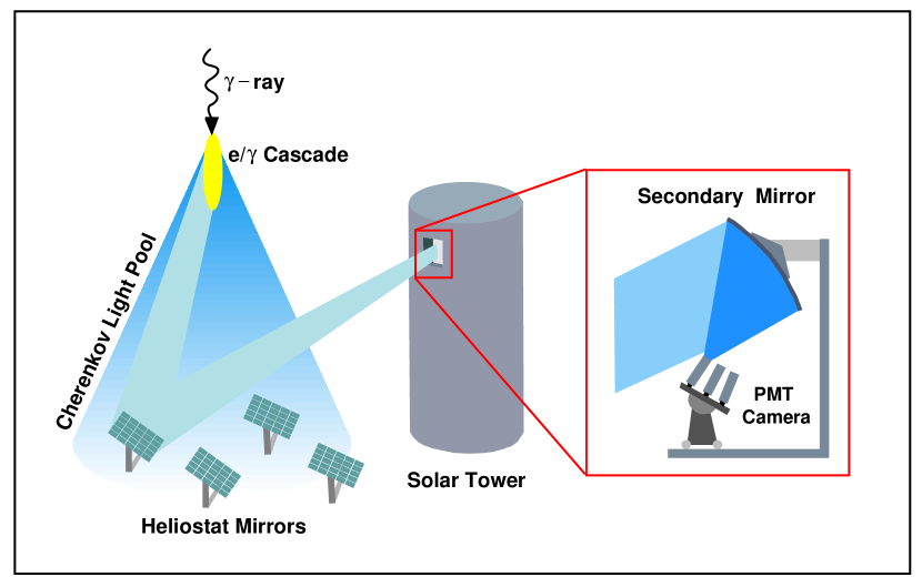
Figure 1: An illustration of the concept behind the STACEE gamma-ray detector. An incident gamma ray produces an air shower and the particles therein generate Cherenkov light. Heliostats on the ground direct this light towards a tower. Secondary mirrors on the tower focus this light onto nearby photomultiplier tubes. Each PMT views a unique heliostat.

STACEE makes use of the large steerable mirrors (heliostats) of the National Solar Thermal Test Facility (NSTTF) in Albuquerque, New Mexico. The NSTTF, built for solar power research, has 224 heliostats, each with an area of 37 m², that can direct sunlight onto a tower on the south side of the field. STACEE uses 64 of these heliostats to sample the Cherenkov light pool and direct the light onto secondary mirrors located on the tower. The secondaries focus the light onto cameras, each of which comprise a cluster of photomultiplier tubes (PMTs) such that each PMT views one heliostat. The process is illustrated schematically in Figure 1.

STACEE’s efficiency for detecting optical photons is wavelength-dependent. At wavelengths shorter than 350 nm the acceptance is cut off by the glass of the heliostat mirrors which are aluminized on their rear surface. At longer wavelengths, the quantum efficiency of the PMTs drops to zero between 600 and 700 nm. Thus STACEE’s sensitivity is best between 400 and 500 nm and peaks at about 420 nm. Such a response is quite suitable for detecting Cherenkov light, but it limits the range of possibilities for detection of interstellar laser pulses. The main concern is that extinction due to absorption and scattering will be greater at shorter wavelengths ($A_{\lambda}/E(B-V)\simeq 3.5$ at $\lambda=420$ nm (Zagury 2001)) and might render a possible signal too weak to see over a realistic distance. With the use of interstellar reddening maps  (Schlegel et al., 1998) it can be shown that such an effect would amount to a loss of 10 to 20% of the beam intensity from sources in the directions of our targets. However, it can still be argued that a longer wavelength would be preferred, and we run the risk that this would be the choice of an advanced civilization.

Pulses from each PMT are amplified and then split, one copy of which is sent to trigger electronics, the other to an 8-bit 1 gigasample/s flash-analog-to-digital converter (FADC). The trigger copy is discriminated and dynamically delayed to account for the the observing geometry since arrival times of Cherenkov light on each heliostat depend on the elevation and azimuth of the source being tracked. Delayed pulses from the different channels are combined and a minimum multiplicity is required within a coincidence window typically 12 ns wide. The FADC data are written to a buffer and when a trigger is generated, a 192 ns portion of this buffer is saved to a data file. Thus the data file consists of a series of events, each of which contain 64 192-ns traces.

More details of the STACEE detector can be found elsewhere  (Chantell et al., 1998; Hanna et al., 2002; Gingrich et al., 2005).

3 Use of STACEE for OSETI

The potential of STACEE as a detector that is well suited to OSETI observations has been described elsewhere (Covault, 2001). Because of its large mirror area, STACEE is potentially more sensitive than detectors based on conventional telescopes (Howard et al., 2004; Stone et al., 2005). Other atmospheric-Cherenkov detectors have already been used in a limited way for OSETI (Holder et al., 2005) or are under consideration for future studies (Armada et al., 2004).

While it is true that, with 64 heliostats, each with an area of 37 m², STACEE has over 2300 m² of collection area for OSETI studies, this has to be balanced with its large field-of-view (FOV) of about 0.6 degrees. This is a design feature, since sensitivity to Cherenkov light from air showers requires an FOV of about this size. This means that, though STACEE is sensitive to low-intensity laser pulses, the air showers it detects provide a background that does not affect the optical-telescope detectors. Thus, the many PMT channels of STACEE cannot be used independently to increase effective area; they must be used together to reject background from air showers generated by high-energy gamma rays and by (the far more copious) charged cosmic rays.

There are several criteria for rejecting backgrounds from air showers, the most powerful of which are uniformity and multiplicity. A laser pulse from a distant source will uniformly illuminate the heliostat field, so we would expect every PMT channel in the STACEE detector to report the same number of photons, though with deviations due to Poisson fluctuations and channel-to-channel efficiency differences.

4 Observations

4.1 OSETI Data Runs

The data presented here were acquired between January and May 2007. During this time, STACEE was being run largely to complete a data set on the active galactic nucleus 1ES 1218+304 (Mukherjee et al., 2007). During the observing hours when this source was not near transit, we kept the detector operational and staffed in order to be ready to follow up gamma-ray burst (GRB) alerts. We used these stand-by hours for a series of 10-minute OSETI observations on a list of candidate stars.

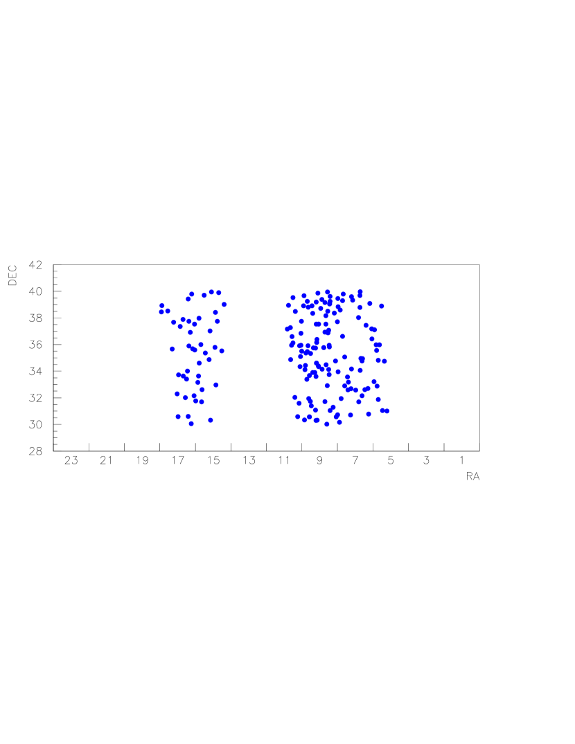
Figure 3: Declination (in degrees) vs right ascension (in hours) for the stars observed during the STACEE OSETI campaign. The space of possibilities was limited by the requirement that the stars transit close to zenith.

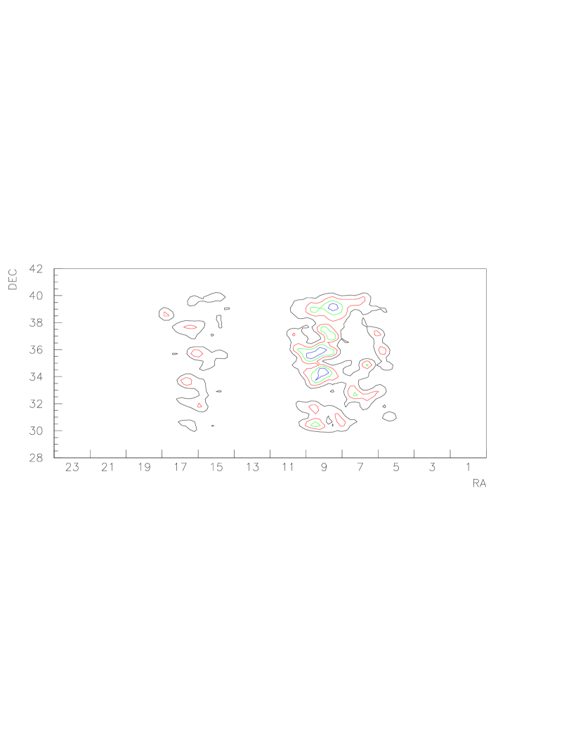
Figure 4: Contour plot of sensitivity as a function of target direction. The positions of the stars plotted in Figure 3 have been smeared with a Gaussian function having a full-width corresponding to the STACEE field-of-view (approximately 0.6 degrees). The contour step size is 20% of the peak sensitivity.

We selected stars from the HabCat catalog (Turnbull and Tarter, 2003), a list of nearby Sun-like stars that conceivably harbor habitable planets. The targets chosen for STACEE were those that would be near zenith when they transited, since the optics of STACEE are optimal for sources overhead. All told, we observed 187 stars. A histogram of their distances from Earth is shown in Figure 2. The celestial coordinates of the stars are plotted in Figure 3. The Hipparcos catalog identifier of each star and the date on which it was observed is listed in Table 1. We note that the FOV of STACEE is approximately 0.6 degrees so there is also sensitivity to any sources located in interstellar space in the region of the targeted stars. (It has been argued (dyson, Dyson, 1959) that advanced civilizations might inhabit “Dyson Spheres” which completely enclose their host stars and are therefore not associated with visible stars. This hypothesis was originally put forward in support of the notion of looking for extraterrestrials at infrared wavelengths. However it does not exclude the possiblility that such beings could be sending out laser pulses of the type we can detect.) In regions between closely-spaced stars the effective sensitivity is increased since that region of space is observed for a longer time. This is quantified in Figure 4 where the points from Figure 3 have been smeared with a Gaussian function with full-width of 0.6 degrees. The contours represent steps of 20% of the peak sensitivity.

The data were acquired via the standard STACEE trigger system, which was configured for GRB follow-up observations. We used this trigger for the OSETI runs to have the capability to switch quickly to GRB observations, with a minimum number of changes, following any alert from the network. For OSETI running the discriminator threshold for each PMT was set at 90 mV, which corresponds to approximately 9 photoelectrons.

4.2 Optical Throughput Measurements

Almost all STACEE triggers result from air showers caused by charged cosmic rays and a small number arise from gamma-ray events. In both cases, a pool of Cherenkov light is distributed over the heliostat field and this pool has a characteristic structure in space and time. Typically there will be systematic differences from channel to channel in the amount of light received and its time of arrival. Thus a very powerful discriminant against air showers is the requirement that every PMT channel report a pulse size consistent with the arrival of a uniform flux of optical photons. To apply such a criterion it is necessary to unfold detector effects, two of which are geometric acceptance and electronic gain. The gains of the PMTs and their amplifiers are equalized with a laser calibration system (Hanna and Mukherjee, 2002) but the efficiencies of the optical components (heliostats, secondary mirrors and light concentrators) also need to be accounted for. As described elsewhere (Hanna et al., 2002), the effective FOV of each heliostat depends on its distance from the tower, and the channel-to-channel differences are roughly compensated for by using optical concentrators with different angular acceptances attached to the PMTs. Additionally, collection of light from the heliostats has slight channel-dependent variations. For example, the PMT cameras occult some of the light from the heliostats, with the exact amount depending on the particular heliostat.

Fortunately, we can directly measure the net result of these effects by performing drift scans on bright stars. We point the heliostats to a location that matches the declination of a star and is four minutes ahead of it in right ascension. We disable heliostat tracking so that each mirror is held in a fixed position. We record photocurrents for eight minutes as the star drifts through the FOV of each PMT channel. Sample plots from the first eight PMT channels are shown in Figure 5. In this figure we plot FADC baseline variance vs time. (The baseline variance is linearly related to photocurrent but its channel-to-channel calibration is more precisely known than that for the photocurrent.) As the star drifts into the field-of-view, the current rises to a maximum and then returns to its quiescent value. The curve is usually asymmetric due to details of the geometry of the heliostat position and the corresponding PMT.

We calculate the difference between the current at the four-minute mark and the average of the currents for the first and last 30 seconds of the scan and use this quantity to define the throughput for the PMT channel. Note that in some cases the maximum deviation does not occur precisely at four minutes because of a slight mis-pointing of the heliostat. For the throughput calculation, however, it is important to use the value at four minutes since that takes into account the effect of the slight mispointing, which will also be present during OSETI runs.

This method of estimating net throughput is quite powerful. Since the photocurrent depends linearly on the number of photoelectrons arriving at the first dynode in the PMT, we automatically account for quantum efficiency and collection efficiency in the PMT, as well as gains in the electron multiplier structure and in the downstream amplifiers. This is in addition to the geometric effects of light collection, reflection and occultation.

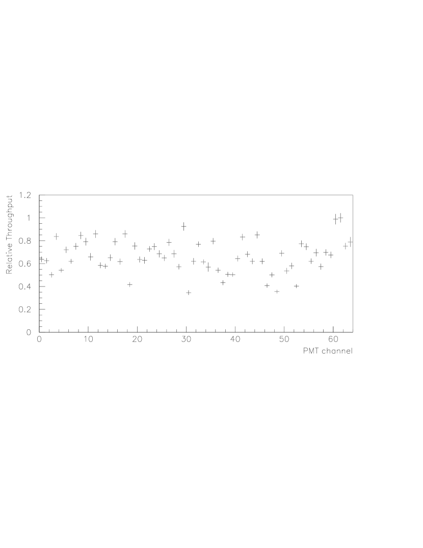
Figure 6: Relative throughputs vs PMT channel number as measured by the drift scan technique.

After calculating a throughput for each PMT channel, the values are scaled such that the channel with the largest throughput has unity value. The relative throughputs are shown in Figure 6. Most channels are within a factor of two of the most efficient one and all are within a factor of three.

4.3 Optical Throughput Calculations

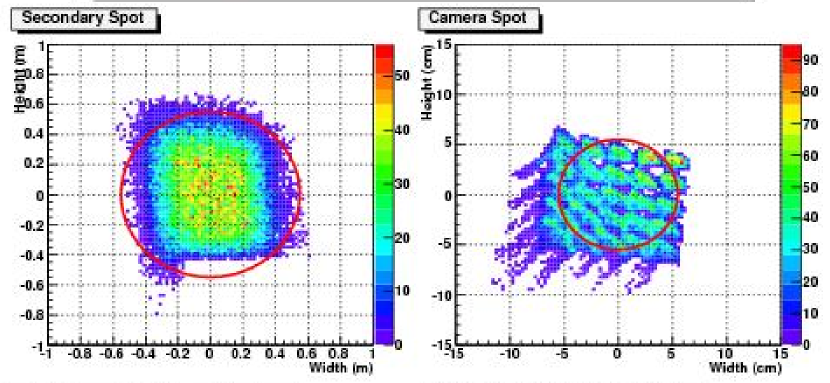
Figure 7: Results for PMT channel 49 from the ray-tracing program used to evaluate absolute throughput. Left panel: impact points of photons at the plane of the secondary mirror. The 2-m circle indicates the position of the mirror. The blank area at the lower right is caused by occultation from the camera structure. Right panel: photon impact positions at the entrance to the optical concentrator on the PMT. Comatic aberration as well as structure due to the heliostat facets can be seen.

The drift scans are well-suited for measuring relative response from channel to channel, but they cannot be used to determine the absolute optical throughput. To do this we use a ray-tracing program that models all the optical components using measured quantities such as reflectivities and transmissions. An indication of the detail of the ray-tracing program is given in Figure 7, which shows the results of tracing the trajectories of photons that arrive vertically onto the heliostat field. The left panel shows the impact points of photons at the secondary mirror on the tower. The outline of this mirror is shown as a circle and the blank region in the lower part is caused by occultation from the camera structure. In the right panel, impact points at the focal plane are shown; the circle corresponds to the entrance aperture of the optical concentrator. Aberration due to coma, as well as the structure caused by the 25 facets of the heliostat can be seen.

Using the ray-tracing program we calculate an average effective area per heliostat of approximately 3 m² at a wavelength of 420 nm. The effective areas range from 1.5 m² to 3.5 m². At 1.5 m² a relatively large amount of light is lost due to occultation and the mis-match between the heliostat image size and the optical concentrator acceptance; at 3.5 m², such losses are less severe. As noted above, the nominal area of each heliostat is 37 m², so the overall efficiency is less than 10%. Most of this is due to the quantum efficiency of the PMTs.

4.4 STACEE Sensitivity

To calculate the optical fluxes to which STACEE would be sensitive, we used a simple Monte Carlo program to simulate the response of our detector to uniform light pulses. Fluxes (in photons/m²) were simulated over a range of values, and the mean numbers of photons expected in each PMT channel were calculated via the optical throughputs obtained from the drift scans. The PMT channel with the best throughput was assigned an effective area of 3.5 m², and the other channels were scaled accordingly. The resulting mean values for the expected numbers of detected photons were used to generate a characteristic Poisson distribution for each PMT channel. 64-channel events were generated by sampling these distributions and the number of detected photons in each channel was corrected for the relative acceptance of the channel. Thus the mean corrected photoelectron count should be the same for all channels but the fluctuations depend on the relative acceptances of the PMT channels. An event was accepted if all channels had a corrected photoelectron count above threshold. Results of this calculation are shown in Figure 8 where efficiency as a function of flux level is plotted for four different threshold values. For typical thresholds, the detector is sensitive to fluxes of the order of 10-15 photons/m². This is very much a wavelength-dependent statement; these calculations were carried out assuming a laser wavelength of 420 nm. For longer wavelengths our sensitivity is less, due to the fall-off in quantum efficiency of the PMTs.

5 Data Analysis

Each data run resulted in a file that contained approximately 1500 events, each of which comprised 64 FADC traces, each 192 samples long. The FADCs used an 8-bit digitizer so that each sample corresponded to a number from 0 to 255. A typical FADC trace consisted of a fluctuating baseline, with an average value of about 220 counts, with a negative-going pulse between sample numbers 80 and 120. Ancillary data such as the time of each event, as read from a GPS clock, made up the rest of the data file.

The data analysis program was designed to re-apply the trigger criterion with tighter timing windows and select events with acceptance-corrected pulses which were consistent, allowing for Poisson fluctuations, with coming from a uniform flash of light. The data processing was done in four stages.

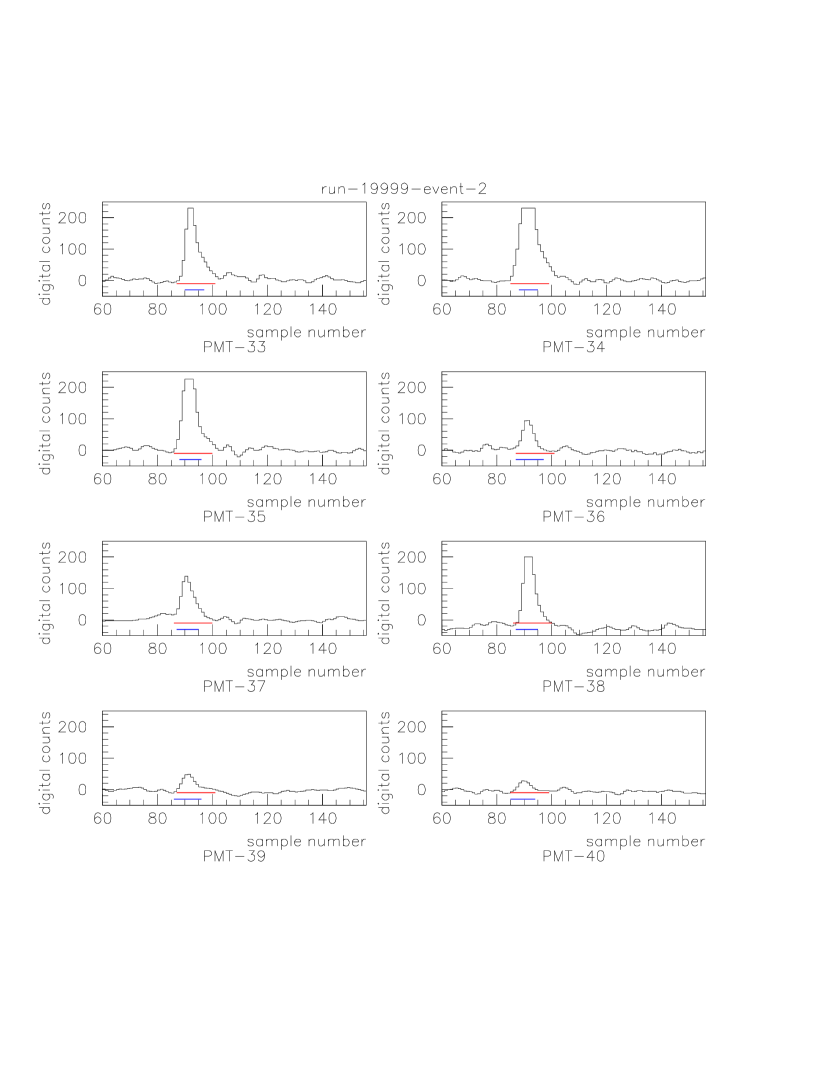
Figure 9: Sample traces from eight PMT channels of a particular event. The channel numbers are shown below each trace. Samples 61 through 156 (of a possible 192 saved samples) are displayed. The upper line shows the range over which the pulse is integrated to give an estimate of the charge. The lower line below indicates the window used in searching for a valid pulse. Although the window for the pulse search can vary from channel to channel, the integration gate is fixed at 15 ns. Note that the flat tops of the traces for channels 34 and 35 are due to saturation.

In the first stage, the first 50 FADC samples for each PMT channel were histogrammed and fit to a Gaussian distribution. The mean was saved as the pedestal for the channel and the root-mean-square standard deviation was saved to be used in defining a cut threshold. The early part of the trace was used to avoid biases from in-time pulses. After the pedestal was computed, it was subtracted and the trace was inverted. (See see Figure 9 for an example of typical traces.) Any channel with at least one sample in its trace above a cut of 3 standard deviations (typically 15-20 counts) was deemed to be hit. If, in the raw trace, any samples were at zero (i.e., the pulse had “bottomed out”) the channel was labelled as saturated (indicating a light level beyond the dynamic range of the digitizer).

In the second stage, hit but unsaturated PMT channels were used to calculate an event time. Channels with maximum sample size more than 50 counts above baseline were used for timing, with the time of the maximum sample used as the time of the pulse. The average of these times from all available channels was used as the event time; due to details of the trigger, this fluctuated by order 10 ns from event to event. The deviation from event time for each channel was histogrammed and fit, at the end of the run, to a Gaussian to define a timing window (mean plus or minus 2.5 standard deviations) for use in the following stage. The width of the timing window so defined was channel-dependent with most channels having a width of 10 ns, though some at the far edge of the heliostat field had windows that were 25 ns wide. The use of narrow, channel-specific search windows enabled the use of the lowest possible thresholds in looking for valid pulses.

In the third stage, the event time and the window limits were used to define a search region for each PMT channel. The maximum sample within the window was used to define the peak of the pulse and the pulse charge was computed by summing the 15 samples starting 5 samples before this point. The channel was counted as hit if the maximum sample was above the cut value defined above. (Note that a channel defined as hit in the second stage of the analysis could lose this status at this point because the above-threshold sample in stage 2 was from outside the search window.) This procedure produced a charge for all channels, even those that were below trigger threshold.

The analysis can be summarized while viewing Figure 9. Displayed in this figure are traces from eight FADC channels for an arbitrary event. The central portion of each trace (samples 61 through 156) is displayed in the figure. The upper line below each pulse delineates the 15 ns integration window used for charge estimation. The lower line indicates the range over which samples are searched for a pulse.

For events with at least 55 PMT channels that have a sample above threshold in the search window, all 64 integrated charges were saved in a file for further processing. Although the signature of a laser pulse would be 64 hit channels, the cut at 55 allows for dead channels in some runs, as well as Poisson fluctuations on low-intensity candidates.

For the selected events, charges were converted from units of counts-ns to photoelectrons with a scale factor of 20 counts-ns per photoelectron. This factor was determined via special calibration and gain-equalizaton runs made with the laser calibration system (Hanna and Mukherjee, 2002). Gaussian ($\sqrt{N}$) uncertainties, which are statistically adequate for $N>10$, were assigned to the photoelectron estimates at this point. The photoelectron estimates and their uncertainties were multiplied by the relative throughput corrections (Figure 6). Using only PMT channels that reported a corrected photoelectron count of at least 10, we computed an average number of photoelectrons for the event. The threshold was applied to avoid including channels that, for some reason were not functioning properly during the run. (On some occasions one or two heliostats were stowed due to mechanical problems.) If an event passed further selection cuts, the low-charge channels could be included in the calculations after checking on the hardware status. Typically, more than 50 channels contributed to the average photoelectron calculation.

To search for events consistent with uniform light illumination, we characterize the extent to which the measured flux in all PMT channels is statistically consistent with a single value. We define a standard chi-squared statistic to characterize the extent to which channels deviate from the the average value. The chi-square per degree-of-freedom ($\chi^{2}_{DOF}$) for such a large number of statistically independent channels should be very strongly peaked at a value of 1.0 for events that are consistent with uniform illumination. Events with ($\chi^{2}_{DOF}$) significantly greater than 1.0 are considered to be non-uniform, and are tagged as air showers. For example, for n=50 the distribution expected for laser pulses is approximately normal with a standard deviation of 0.3. Events with $\chi^{2}_{DOF}<2.0$ were individually checked. An example of data from such an event is shown in Figure 10. The corrected number of photoelectrons for each of the 64 PMT channels is plotted vs channel number, along with the fitted average. Figure 11 shows the mean charge (in counts-ns) vs channel number for all events in the run. The uneven structure is caused by the distribution of Cherenkov light in air showers and the efficiency for triggering on such showers as a function of where they hit the heliostat field. The fact that no channels reported zero for mean charge indicates that they were all in good working order for this run. This result indicates that the zeros in PMT channels 45-48 in Figure 10 are due to a lack of light in the corresponding heliostats. This is not unexpected in air-shower events.

The distribution of $\chi^{2}_{DOF}$ for all fits in the run is shown in Figure 12. Most runs have one or two events that have $\chi^{2}_{DOF}<2.0$ at this stage. These are invariably rejected because they have PMT channels that have below-threshold pulse sizes (often zero) even though the mean-charge distributions indicate that they are in good working order. These small pulses were left out of the initial average and $\chi^{2}_{DOF}$ calculation because of the 10-photoelectron threshold designed to accomodate possibly bad channels. When they are included, the $\chi^{2}_{DOF}$ gets much larger.

As can be seen in Figure 8, with the 10-photoelectron threshold used in the analysis, we were fully efficient for flashes that resulted in flux levels above 10 photons/m² at the detector. After processing all the data runs, we did not have any candidates consistent with the arrival of pulses of at least this intensity.

6 Discussion

In the field of elementary particle physics, searches for new particles and related phenomena are common. Examples include the hunt for the weak interaction bosons (W and Z), the top quark and neutrino oscillations. These searches were ultimately successful. Presently ongoing searches include the quest for axions, the Higgs boson, and dark matter particles such as WIMPs. In such searches there is a space of possibilities with coordinates such as particle mass and interaction cross-section. Null results are presented as exclusion plots, which indicate what parts of the parameter space have been ruled out in that they do not warrant further consideration. Progress is made by shifting the boundaries of these excluded regions into unexplored regions.

OSETI searches are not so systematic. It is possible to imagine repeating the same experiment some time after it was first carried out and obtaining different results. A null result could be changed to a positive result in the event a distant civilization has, in the interim started sending out detectable signals. Repeating the experiment with a slight change in one aspect, e.g., dwell time on the target, might lead to a successful detection.

What did we learn from the results of our search with the STACEE detector? We can say that blue-green laser pulses of detectable intensity were not being sent, in our direction and from the vicinity of the target star, within those 10-minute intervals during which our search was directed at them. Saying more is difficult.

Instrumentally, we have learned that use of a heliostat array for OSETI searches is possible. However the large mirror area is reduced to a much smaller effective area by the quantum efficiency of the PMTs and various geometric factors. The wavelength range is rather small and this reduces the amount of parameter space that can be investigated, though this shortcoming could be reduced with PMTs chosen for OSETI rather than Cherenkov astronomy.

The large number of heliostats cannot be used to synthesize a giant collector, and, thereby, increase sensitivity to faint laser pulses. This is because multiple channels are needed to reject the huge background of nanosecond optical flashes caused by extensive air showers. The simple analysis described in this paper requires a larger photon flux than the 2 photons/m² foreseen by Covault (2001) but it is not excluded that, using techniques described in that paper (fitting the times to a wavefront, cutting on arrival direction, etc.), one could lower the required flux.

The loss of effective collection area is offset somewhat by the larger field-of-view afforded by an instrument of this type. We have not explored how few channels can be used to suppress Cherenkov background sufficiently, but it could be possible to divide the detector into several smaller detectors to allow for several regions to be monitored at once This would require more electronics to construct the extra triggers.

How does the STACEE search compare to other OSETI efforts?

The Harvard-Princeton search  (Howard et al., 2004) was much more extensive, with nearly 16,000 observations on over 6000 objects totalling 2400 hours of data. The typical time per target was 24 minutes. The stated sensitivity was 100 photons/m² in a window of 5 ns in the 450-650 nm band for the Harvard telescope. The Princeton telescope, which observed in parallel for 1142 of the targets, had a similar sensitivity (80 photons/m²).

A team at the Lick Observatory made 5000 targeted observations with use of a conventional optical telescope (Stone et al., 2005). Their flux sensitivity was similar, but their time-on-target was 10 minutes.

The Harvard all-sky-detector team (Howard et al., 2007) reported that they achieved a sensitivity of 95 photons/m² in a window of 3 ns. They ran in a drift-scan mode with a consequent one-minute dwell time per source point.

A group  (Holder et al., 2005) searching for OSETI signals in archival data from the Whipple 10-meter gamma-ray telescope, another Cherenkov-based instrument, demonstrated that a sensitivity of 10 photons/m² is possible. Each run in their search had a length of 28 minutes, but the same part of the sky was targeted in many different runs since gamma-ray observations typically require very long exposures. Because of this the total time spent on a given target was very large.

One conclusion from this comparison is that the large mirror areas of the Cherenkov telescopes can be used to improve flux sensitivity by about one order of magnitude compared with the smaller optical telescopes. To put the flux of 10 photons/m² in perspective, we consider a 400 nm laser at a distance of 1000 light years. A 0.3 MJ pulse would contain $6\times 10^{23}$ photons, and if these were formed into a diffraction-limited beam with a 10 m mirror, the beam diameter at the Earth would be $4\times 10^{11}$ m. Assuming that the profile is such that half the photons fall within a diameter of $2\times 10^{11}$ m, an average flux density of 10 photons/m² is obtained. Lasers with an order of magnitude greater pulse energy have already been developed, so our search is not limited by what might be considered reasonable technical achievements of distant civilisations.

7 Future Progress

The STACEE detector was dismantled during the summer of 2007 so there will be no further observations of the type reported here. Some members of the STACEE collaboration, however, have been studying the possibilities for future detectors dedicated to OSETI. One idea that has emerged is the concept of multiple, distributed OSETI detectors.

This idea foresees the use of a large number of inexpensive detectors, each of which carry out drift scans in the manner of the Harvard all-sky detector (Howard et al., 2007). A detector element would consist of two pairs of telescopes, where each telescope comprises a simple spherical mirror, approximately one meter in diameter, with a single PMT at the focus. The two members of a pair, both pointing at the zenith, would be located on the order of 100 meters apart and operated in coincidence mode with cables and simple electronics. With each local coincidence, digitized pulses from the two PMTs would be stored along with a GPS time stamp. Most of these recorded events would be due to Cherenkov light from large air-showers, but the rate would not be large due to the separation of the two members of the pair. A second, identical pair directed at the same spot on the sky would be deployed several kilometers away such that coincidences between the two pairs could not be caused by air-showers. Data from the two pairs would be compared off-line using the GPS time stamps to identify coincidences and the digitized pulses to check for uniform illumination.

A large number of such installations could be built, possibly in the style of the various outreach projects involving cosmic-ray detectors located at high schools (Carlson et al., 2004). With a large number of detectors, each scanning the same strip of sky night after night, one would address what we consider to be one of the most important limitations of the OSETI searches carried out to date: duty factor. It is important to be live and on-target when a distant laser is pointed our way. Sensitivity to faint laser pulses would not be useful if the laser and detector were not co-aligned at the crucial time. A world-wide grid with spacing on the order of the detector field-of-view would be useful and affordable, given the simple nature of the detectors, which involve very basic electronics and no moving parts.

Of course, the success of an OSETI campaign would depend on whether civilizations exist that have the impetus to transmit laser pulses. The number of such civilizations cannot be estimated reliably, though limits can be set by using tools such as the Drake equation (Drake, 1992). This equation attempts to identify the various factors needed to make such an estimate, so that some of the uncertainties involved can be quantified. Hetesi and Regály (hetesi, 2006) purported that the Drake equation is not complete in that it neglects certain key factors, e.g., advanced civilisations may choose to remain silent. There are many good reasons to suspect that such civilisations would be in the majority.

8 Conclusion

We have used the STACEE high-energy gamma-ray detector to look for fast blue-green laser pulses from the vicinity of 187 stars. These stars have been chosen because their characteristics are such that they may harbor habitable planets and they are relatively close to Earth. Each star was observed for 10 minutes, and we found no evidence for laser pulses with intensities greater than about 10 photons/m² at 420 nm in any of the data sets.

9 Acknowledgements

We are grateful to the staff at the National Thermal Solar Test Facility for their enthusiastic and professional support. The STACEE project was funded in part by the U.S. National Science Foundation, the University of California, Los Angeles, the Natural Sciences and Engineering Research Council, le Fonds Québecois de la Recherche sur la Nature et les Technologies, the Research Corporation, and the California Space Institute.

Figure 2: Histogram of the distances to the 187 stars observed during the STACEE OSETI campaign.

Figure 5: FADC baseline variances (in digital-counts-squared) vs time (in minutes) for a drift scan with a bright star. Each plot corresponds to a different PMT channel. The deviation of the trace at 4 minutes from the baseline value is a relative measure of the net throughput of the channel.

Figure 8: Efficiency vs optical flux levels for the STACEE detector for four threshold values. An effective area of 3.5 m² for the most efficient PMT channel has been assumed and all other channels have been scaled according to the relative throughputs plotted in Figure 6. Using a 10-photoelectron analysis threshold, we find no candidate laser flashes in the STACEE data.

Figure 10: Example of an event singled out for attention during the final stage of analysis. The corrected pulse size (in photoelectrons) is plotted vs PMT channel number, together with the average computed using channels reporting more than 10 photoelectrons. The $\chi^{2}_{DOF}$ for this event is 1.64.

Figure 11: Mean charge vs PMT channel number for the run containing the candidate event shown in Figure 10. Units are counts-ns. The structure is due to array geometry, trigger effects, and the distribution of light from air showers. The fact that each channel reports a non-zero mean value indicates that there were no defective channels in this run.

Figure 12: Distribution of $\chi^{2}_{DOF}$ for the events in the run containing the event in Figure 10.

Table 1: Target Stars: the identifier refers to the Hipparcos Catalog and the Observation date is month and day in 2007.

Identifier	Observed	Identifier	Observed	Identifier	Observed	Identifier	Observed
41998	0124	36053	0217	47993	0222	76859	0317
42686	0124	37374	0217	49770	0222	78751	0317
41930	0124	38995	0217	71753	0223	79538	0317
45334	0124	39112	0217	72892	0223	80206	0317
47313	0124	39459	0217	72175	0223	81147	0317
46033	0125	41530	0217	74260	0223	82432	0317
47016	0125	42445	0217	44502	0312	36952	0318
43596	0125	42763	0217	45883	0312	37991	0318
43895	0125	42405	0217	46707	0312	38950	0318
45126	0125	45175	0217	48202	0312	41382	0318
45307	0125	46446	0217	48465	0312	41888	0318
32304	0213	25614	0218	49283	0312	43024	0318
34809	0213	26863	0218	50920	0312	44502	0318
34977	0213	27361	0218	49241	0312	45053	0318
36904	0213	28102	0218	51454	0312	45006	0318
38480	0213	29617	0218	52885	0312	46993	0318
26506	0216	30391	0218	44646	0314	72628	0319
28005	0216	32168	0218	48566	0314	73829	0319
27234	0216	32239	0218	49157	0314	74512	0319
28707	0216	32211	0218	51804	0314	75579	0319
29319	0216	33557	0218	52601	0314	76525	0319
29874	0216	35193	0218	52119	0314	77402	0319
31619	0216	34812	0218	41382	0316	78638	0319
31431	0216	35825	0218	41642	0316	80326	0319
34468	0216	38295	0218	43471	0316	72760	0320
35962	0216	38949	0218	45006	0316	74156	0320
37620	0216	39667	0218	45162	0316	75908	0320
37589	0216	41292	0218	46993	0316	76656	0320
39031	0216	42386	0218	48387	0316	78277	0320
40037	0216	41270	0218	49529	0316	78559	0320
41272	0216	42730	0218	49687	0316	80807	0320
41521	0216	44525	0218	49111	0316	77469	0416
42104	0216	45484	0218	50767	0316	77670	0416
41691	0216	46314	0218	52052	0316	79381	0416
44987	0216	47413	0218	77304	0316	80571	0416
44559	0216	40398	0221	79105	0316	80128	0416
24295	0217	41454	0221	79824	0316	81677	0416
25030	0217	41888	0221	80417	0316	83075	0416
25852	0217	42182	0221	81776	0316	84283	0416
26849	0217	43024	0221	82938	0316	83326	0416
27501	0217	44856	0221	45196	0317	84688	0416
28727	0217	45053	0221	47739	0317	85879	0416
30751	0217	47581	0221	48081	0317	87526	0416
31972	0217	47191	0221	50185	0317	70297	0420
31576	0217	46636	0222	49358	0317	70930	0420
32658	0217	46022	0222	51460	0317	87680	0420
32568	0217	47575	0222	51687	0317

References

- Armada et al. (2004) Armada, A., Cortina, J. and Martinez, M. (2004) Optical SETI with MAGIC, In Neutrinos and Explosive Events in the Universe, edited by Maurice M. Shapiro, Todor Stanev and John P. Wefel, Springer pp 307-310.
- Bhathal (2001) Bhathal, R. (2001) Optical SETI in Australia, In Proceedings SPIE 4273: The Search for Extraterrestrial Intelligence (SETI) in the Optical Spectrum III, edited by S.A. Kingsley and R. Bhathal, SPIE, Bellingham, WA, pp 144-152.
- Carlson et al. (2004) Carlson, B.E., Brobeck, E., Jillings, C.J., Larson, M.B., Lynn, T.W., McKeown, R.D., Hill, James E., Falkowski, B., Seki, R., Sepikas, J., Yodh, G.B. (2005) Search for Correlated High Energy Cosmic Ray Events with CHICOS Journal of Physics G31, pp 409-416.
- Chantell et al. (1998) Chantell M.C., Bhattacharya D., Covault C.E., Dragovan M., Fernholz R., Gregorich D.T., Hanna D.S., Marion G.H., Ong R.A., Oser S., Tumer T.O., Williams D.A. (1998) Prototype Test Results of the Solar Tower Atmospheric Cherenkov Effect Experiment (STACEE), Nuclear Instruments and Methods A408 pp 468-485.
- (5) Cocconi, G. and Morrison, P. (1959) Searching for Interstellar Communications, Nature 184, 844.
- Covault (2001) Covault, C.E. (2001) Large Area Solar Power Heliostat Arrays for OSETI, In Proceedings SPIE 4273: The Search for Extraterrestrial Intelligence (SETI) in the Optical Spectrum III, edited by S.A. Kingsley and R. Bhathal, SPIE, Bellingham, WA, pp 161-172.
- Drake (1992) Drake, F., Sobel, D. (1992). Is Anyone Out There? The Scientific Search for Extraterrestrial Intelligence. New York: Delacorte Pr. ISBN 0-385-30532-X.
- (8) Dyson, F.J. (1959) Search for artificial stellar sources of infrared radiation, Science 131, pp 1667-1668.
- Gingrich et al. (2005) Gingrich, D.M., Boone, L.M., Bramel, D., Carson, J., Covault, C.E., Fortin, P., Hanna, D.S., Hinton, J.A., Jarvis, A., Kildea, J., Lindner, T., Mueller, C., Mukherjee, R., Ong, R.A., Ragan, K., Scalzo, R.A., Theoret, C.G., Williams, D.A., Zweerink, J.A.,(2005), The STACEE Ground Based Gamma-ray Detector, IEEE Transactions on Nuclear Science 52: pp 2977-2985.
- Hanna et al. (2002) Hanna, D.S., Bhattacharya, D., Boone, L.M., Chantell, M.C., Conner, Z., Covault, C.E., Dragovan, M., Fortin,P., Gregorich, D.T., Hinton, J.A., Mukherjee, R., Ong, R.A., Oser, S., Ragan, K., Scalzo, R.A., Schuette, D.R., Theoret, C.E., Tumer, T.O., Williams, D.A., Zweerink J.A.,(2002), The STACEE-32 Ground Based Gamma-ray Detector, Nuclear Instruments and Methods A489: pp 126-151.
- Hanna and Mukherjee (2002) Hanna, D.S. and Mukherjee, R., (2002) The Laser Calibration Sysyem for the STACEE Ground-based Gamma-ray Detector, Nuclear Instruments and Methods A482: pp 271-280.
- (12) Hetesi, Z. and Regály, Z., (2006) A New Interpretation of Drake-Equation, JBIS 59, pp 11-14.
- Holder et al. (2005) Holder, J., Ashworth, P., LeBohec, S., Rose, H.J., Weekes, T., (2005) Optical SETI with Imaging Cherenkov Telescopes, in Proceedings of the 29th International Cosmic Ray Conference, Pune 5, pp 387-390.
- Howard et al. (2004) Howard, A.W., Horowitz, P., Wilkinson, D.T., Coldwell, C.M., Groth, E.J., Jarosik, N., Latham, D.W., Stefanik, R.P., Willman, A.J.Jr., Wolff, J., Zajac, J.M., (2004) Search for Nanosecond Optical Pulses from Nearby Solar-Type Stars, Astrophysical Journal 613, pp 1270-1284.
- Howard et al. (2007) Howard, A.W., Horowitz, Mead, C., Sreetharan, P., Gallicchio, J., Howard, S., Coldwell, C., Zajac, J., Sliski, A., (2007), Initial resulsts from the Harvard all-sky optical SETI, Acta Astronautica 61, pp 78-87.
- Mukherjee et al. (2007) Mukherjee, R., Akhter, N., Ball, J., Carson, J.E., Covault, C.E., Driscoll, D.D., Fortin, P., Gingrich, D.M., Hanna, D.S., Jarvis, A., Kildea, J., Lindner, T., Mueller, C., Ong, R.A., Ragan, K., Williams, D.A., Zweerink, J.A., (2007), STACEE Observations of 1ES 1218+304, in Proceedings of the 30th International Cosmic Ray Conference, Merida.
- Schlegel et al. (1998) Schlegel, D., Finkbeiner, D., and Davis, M., Maps of dust infrared emission for use in estimation of reddening and cosmic microwave background radiation foregrounds. Astrophys. J.500, pp 500-553.
- Stone et al. (2005) Stone, R.P.S, Wright, S.A., Drake, F., Munoz, M., Treffers, R., Werthimer, D., (2005), Lick Observatory Optical SETI: Targeted Search and New Directions, Astrobiology 5: pp 604-611.
- Schwartz and Townes (1961) Schwartz, R. and Townes, C.H. (1961), Interstellar and interplanetary communication by optical masers. Nature 190, 205-208
- Turnbull and Tarter (2003) Turnbull, M.C. and Tarter, J.C. (2003), Target Selection for SETI. II. Tycho-2 Dwarfs, Old Open Clusters, and the Nearest 100 Stars, Astrophysical Journal Supplement 149, pp 423-436.
- Weekes (2006) Weekes, T.C. (2006), Revealing the Dark TeV Sky: The Atmospheric Cherenkov Imaging Technique for Very High Energy Gamma-ray Astronomy, in Proceedings of the International Workshop on “Energy Budget in the High Energy Universe”, Kashiwa, Japan.
- Zagury (2001) Zagury, F., The standard theory of extinction and the spectrum of stars with very little reddening, New Astronomy 6, 471