UdeM-GPP-TH-09-176

Looking for New Physics in $B\to K^{*}\pi$ and $B\to\rho K$ Decays

Cheng-Wei Chiang ^a, and David London ^b,

$a$: Department of Physics and Center for Mathematics and Theoretical Physics,
          National Central University, Chungli, Taiwan 320, Taiwan;
          Institute of Physics, Academia Sinica, Taipei, Taiwan 115, Taiwan
      $b$: Physique des Particules, Université de Montréal,
          C.P. 6128, succ. centre-ville, Montréal, QC, Canada H3C 3J7

$B\to K^{*}\pi$ and $B\to\rho K$ decays involve the same quark-level processes as $B\to\pi K$. Analyzing the measurements of the former decays might be able to shed additional light on the new-physics hints in the current $B\to\pi K$ data. We perform fits to $B\to K^{*}\pi$ and $B\to\rho K$ decays, and find that the data can be accommodated within the standard model. However, this agreement is due principally to the large errors in the data, particularly the CP-violating asymmetries. If the errors on the $B\to K^{*}\pi$ and $B\to\rho K$ observables can be reduced, one will have a clearer sense of whether new physics is present in these decays.

In recent years, experimental data in $B\to\pi K$ decays have shown some discrepancies with the predictions of the standard model (SM), hinting at new-physics (NP) contributions in the decay processes . This so-called $\pi K$ puzzle has received a great deal of attention. The NP presumably enters the short-distance pieces of the decay amplitudes. It should therefore affect other closely-related processes as well. In particular, the final-state $VP$ counterparts of $B\to\pi K$ decays ($V$ is a vector meson, $P$ is a pseudoscalar ) – $B\to K^{*}\pi$ and $B\to\rho K$ decays – involve essentially the same quark-level processes. It is thus of interest to see whether the current experimental data of these decays also present similar hints of NP. (Even within the SM, these decay modes are useful in extracting the weak phase $\gamma$ [5, 6, 7].)

The eight $VP$ decay modes can be readily divided into two sets: (I) $B\to K^{*}\pi$ decays and (II) $B\to\rho K$ decays, each of which involves a different set of flavor amplitudes from the other. As is usually done, in our analysis we neglect the dynamically-suppressed exchange and annihilation amplitudes. In addition, the quantum chromodynamics (QCD) penguin amplitude has three pieces, and can be written as

$$P^{\prime} = V_{ub}^{*}V_{us}{\tilde{P}}^{\prime}_{u}+V_{cb}^{*}V_{cs}{\tilde{P}}^{\prime}_{c}+V_{tb}^{*}V_{ts}{\tilde{P}}^{\prime}_{t}$$ (1)

$$= V_{ub}^{*}V_{us}({\tilde{P}}^{\prime}_{u}-{\tilde{P}}^{\prime}_{c})+V_{tb}^{*}V_{ts}({\tilde{P}}^{\prime}_{t}-{\tilde{P}}^{\prime}_{c})~{}.$$

(The primes on the amplitudes indicate ${\bar{b}}\to{\bar{s}}$ transitions.) In writing the second line, we have used the unitarity of the Cabibbo-Kobayashi-Maskawa (CKM) matrix. In the following, all diagrams (except ${\tilde{P}}^{\prime}_{c}$) are redefined to absorb the magnitudes of the CKM matrix elements which multiply them, i.e., $P^{\prime}_{u}\equiv|V_{ub}^{*}V_{us}|{\tilde{P}}^{\prime}_{u}$, $P^{\prime}_{uc}\equiv|V_{ub}^{*}V_{us}|({\tilde{P}}^{\prime}_{u}-{\tilde{P}}^{\prime}_{c})$, $P^{\prime}_{tc}\equiv|V_{tb}^{*}V_{ts}|({\tilde{P}}^{\prime}_{t}-{\tilde{P}}^{\prime}_{c})$, etc. Because $|V_{ub}^{*}V_{us}|\ll|V_{tb}^{*}V_{ts}|$, it is expected that $|P^{\prime}_{uc}|\ll|P^{\prime}_{tc}|$. To begin with, we keep six types of diagrams: the color-allowed tree, denoted by $T^{\prime}$; the color-suppressed tree, $C^{\prime}$; two QCD penguin amplitudes, $P^{\prime}_{tc}$ and $P^{\prime}_{uc}$; the color-allowed EW penguin, $P^{\prime}_{EW}$; and the color-suppressed EW penguin, $P_{EW}^{\prime C}$. We further use a subscript $P$ or $V$ for each diagram to indicate which final-state meson contains the spectator quark of the $B$ meson.

Explicitly, we have for the decay modes in Set (I):

$$A_{I}^{0+} = -P^{\prime}_{tc,P}+P^{\prime}_{uc,P}e^{i\gamma}+\frac{1}{3}P_{EW,P}^{\prime C}~{},$$

$$\sqrt{2}A_{I}^{+0} = P^{\prime}_{tc,P}-P^{\prime}_{uc,P}e^{i\gamma}+P^{\prime}_{EW,V}-T^{\prime}_{P}e^{i\gamma}-C^{\prime}_{V}e^{i\gamma}+\frac{2}{3}P_{EW,P}^{\prime C}~{},$$

$$A_{I}^{+-} = P^{\prime}_{tc,P}-P^{\prime}_{uc,P}e^{i\gamma}-T^{\prime}_{P}e^{i\gamma}+\frac{2}{3}P_{EW,P}^{\prime C}~{},$$

$$\sqrt{2}A_{I}^{00} = -P^{\prime}_{tc,P}+P^{\prime}_{uc,P}e^{i\gamma}+P^{\prime}_{EW,V}-C^{\prime}_{V}e^{i\gamma}+\frac{1}{3}P_{EW,P}^{\prime C}~{};$$ (2)

and for the decay modes in Set (II):

$$\sqrt{2}A_{II}^{0+} = P^{\prime}_{tc,V}-P^{\prime}_{uc,V}e^{i\gamma}+P^{\prime}_{EW,P}-T^{\prime}_{V}e^{i\gamma}-C^{\prime}_{P}e^{i\gamma}+\frac{2}{3}P_{EW,V}^{\prime C}~{},$$

$$A_{II}^{+0} = -P^{\prime}_{tc,V}+P^{\prime}_{uc,V}e^{i\gamma}+\frac{1}{3}P_{EW,V}^{\prime C}~{},$$

$$A_{II}^{-+} = P^{\prime}_{tc,V}-P^{\prime}_{uc,V}e^{i\gamma}-T^{\prime}_{V}e^{i\gamma}+\frac{2}{3}P_{EW,V}^{\prime C}~{},$$

$$\sqrt{2}A_{II}^{00} = -P^{\prime}_{tc,V}+P^{\prime}_{uc,V}e^{i\gamma}+P^{\prime}_{EW,P}-C^{\prime}_{P}e^{i\gamma}+\frac{1}{3}P_{EW,V}^{\prime C}~{};$$ (3)

In the amplitudes $A_{\alpha}^{ij}$ ($\alpha\in\left\{I,II\right\}$ and $i,j\in\left\{0,+\right\}$) appearing in Eqs. (S0.Ex2) and (S0.Ex5), the subscript $\alpha$ denotes the decay set and the superscripts $ij$ denote the electric charges of the vector and pseudoscalar mesons, respectively. Here we have explicitly written the weak phase associated with each amplitude (including the minus sign of $V_{tb}^{*}V_{ts}$ in the QCD and EW penguins), while the diagrams contain the strong phases.

In fact, there are relations among the various diagrams. The ratios of Wilson coefficients $c_{10}/c_{9}$ and $c_{2}/c_{1}$ are equal, to a good approximation (the difference is only about 3%). In the limit in which this equality is exact, the relations read [5]

$$P^{\prime}_{EW,M} = -\frac{3}{2}{c_{9}\over c_{1}}\left(T^{\prime}_{M}+P^{\prime}_{u,M^{\prime}}\right)~{}~{}~{}~{}M^{\prime}\neq M~{},$$

$$P_{EW,M}^{\prime C} = -\frac{3}{2}{c_{9}\over c_{1}}\left(C^{\prime}_{M}-P^{\prime}_{u,M}\right)~{}.$$ (4)

Now, the diagram $P^{\prime}_{u}$ does not appear in the $B$-decay amplitudes. Thus, in order to use these relations, an approximation must be made. We consider two possibilities. In the first, we neglect all factors of $P^{\prime}_{u}$ and $P^{\prime}_{uc}$. In the second, we replace the $P^{\prime}_{u}$ in the above relations by $P^{\prime}_{uc}$. Both approximations are justified because $|P^{\prime}_{u}|$ and $|P^{\prime}_{uc}|$ are expected to be small. In either case, the relations relate some diagrams appearing in $B\to K^{*}\pi$ decays to some in $B\to\rho K$ decays. That is, the fits must be performed to measurements of both decays simultaneously. We call the fits corresponding to the two approximations Fit1 and Fit2. Also, throughout this paper, the strong phases of the amplitudes are defined with respect to $T^{\prime}_{P}$.

Current experimental measurements of the observables in $B\to K^{*}\pi$ and $B\to\rho K$ decays are given in Table 1. In the first approximation, where $P^{\prime}_{uc}$ is neglected, the direct CP asymmetries ($A_{CP}$’s) of $K^{*0}\pi^{+}$ and $\rho^{0}K^{+}$ are identically zero within this framework. Therefore, it is of no use including them in the $\chi^{2}$ functions as they impose no constraint on the theory parameters. We are then left with 15 and 17 observables in Fit1 and Fit2, respectively.

Set	Mode	BR ($\times 10^{-6}$)	$A_{CP}$	$S_{CP}$
(I)	$B^{+}\to K^{*0}\pi^{+}$	$10.0\pm 0.8$	$-0.020^{+0.067}_{-0.061}$	–
	$B^{+}\to K^{*+}\pi^{0}$	$6.9\pm 2.3$	$0.04\pm 0.29$	–
	$B^{0}\to K^{*+}\pi^{-}$	$10.3\pm 1.1$	$-0.25\pm 0.11$	–
	$B^{0}\to K^{*0}\pi^{0}$	$2.4\pm 0.7$	$-0.15\pm 0.12$	–
(II)	$B^{+}\to\rho^{0}K^{+}$	$3.81^{+0.48}_{-0.46}$	$0.419^{+0.081}_{-0.104}$	–
	$B^{+}\to\rho^{+}K^{0}$	$8.0^{+1.5}_{-1.4}$	$-0.12\pm 0.17$	–
	$B^{0}\to\rho^{-}K^{+}$	$8.6^{+0.9}_{-1.1}$	$0.15\pm 0.06$	–
	$B^{0}\to\rho^{0}K^{0}$	$5.4^{+0.9}_{-1.0}$	$0.01\pm 0.20$	$0.63^{+0.17}_{-0.21}$

Table 1: Branching ratios, direct CP asymmetries $A_{CP}$, and mixing-induced CP asymmetry $S_{CP}$ (if applicable and measured) in $B\to K^{*}\pi$ and $B\to\rho K$ decays. Quoted values are taken from Ref. [8] that weight-averages individual measurements [9, 10, 11, 12, 13, 14, 15, 16, 17, 18, 19, 20, 21, 22].

In both Fit1 and Fit2, one of the theoretical parameters is the weak phase $\gamma$. We have two options in treating it. One possibility is to extract $\gamma$ from the $B\to K^{*}\pi$ and $B\to\rho K$ measurements. This value can then be compared with that obtained from independent measurements [23]:

$$\gamma=(66.8^{+5.4}_{-3.8})^{\circ}~{}.$$ (5)

If the two values of $\gamma$ disagree, this will be a hint of NP. Alternatively, one can impose the value of $\gamma$ of Eq. (5) by adding a constraint to the fits. We perform fits using both of these options. Fit1-a and Fit2-a extract $\gamma$ from the data; Fit1-b and Fit2-b have the additional $\gamma$ constraint (in which the asymmetrical errors are averaged).

In all fits, there will be a hint of NP if the extracted values of the diagrams disagree with the SM calculations. In the QCD factorization (QCDF) approach, the default parameters have the following ratios of amplitudes [24]:

$$|C^{\prime}_{V}/T^{\prime}_{P}|=0.16\pm 0.11~{},\mbox{ and }|T^{\prime}_{P}/P^{\prime}_{tc,P}|=0.59\pm 0.12~{};$$

$$|C^{\prime}_{P}/T^{\prime}_{V}|=0.20\pm 0.13~{},\mbox{ and }|T^{\prime}_{V}/P^{\prime}_{tc,V}|=0.55\pm 0.26~{}.$$ (6)

We begin with Fit1-a. Here, the diagram $P^{\prime}_{uc}$ is neglected. There are therefore a total of 11 hadronic theoretical parameters: 6 amplitude magnitudes, and 5 relative strong phases. In addition, we have the unknown weak phase $\gamma$. Finally, the mixing-induced CP asymmetry $S_{CP}(\rho^{0}K^{0})$ depends also on the weak phase $\beta$. For this, we impose the additional constraint $\beta=(21.66^{+0.95}_{-0.87})^{\circ}$ [23], which is obtained mainly from the measurement of CP violation in $B_{d}^{0}(t)\to J/\Psi K_{\scriptscriptstyle S}$ and other ${\bar{b}}\to{\bar{c}}c{\bar{s}}$ decays. We average the asymmetrical errors on $\beta$. The degree of freedom ($d.o.f.$) is therefore 3 in this fit.

Before presenting the results of this fit, we note the following. There are quite a few solutions, many of which suggest the presence of new physics (NP). While we cannot be absolutely sure that one of these is not the true solution, we make the assumption that the NP, if present, is not enormous. If it were, it probably would already have been seen elsewhere. The large-NP scenarios can be eliminated by demanding that an acceptable solution respect certain constraints on the ratios of magnitudes of diagrams. Now, as we will see, the errors in the fits of the theoretical parameters are quite large. If we consider the full 1$\sigma$ range of these parameters, all potential solutions will respect the constraints. For this reason, we concentrate only on the central values. In particular, we require that the central values of any solution do not violate the ratios of Eq. (S0.Ex9) by a large amount. We impose the conservative constraints

$$|C^{\prime}_{V}/T^{\prime}_{P}|,~{}|C^{\prime}_{P}/T^{\prime}_{V}|\leq 1~{},\mbox{ and }|T^{\prime}_{P}/P^{\prime}_{tc,P}|,~{}|T^{\prime}_{V}/P^{\prime}_{tc,V}|\leq 2~{}.$$ (7)

If any one of these is violated, the solution is excluded. There are a great many possible solutions. But if we restrict $\chi^{2}_{min}$ to be reasonably small, there are only 14. The above constraints eliminate 12 of these.

$\chi^{2}_{min}$	$|P^{\prime}_{tc,P}|$	$|P^{\prime}_{tc,V}|$	$|T^{\prime}_{P}|$	$|T^{\prime}_{V}|$
0.98	$32.9^{+1.5}_{-1.6}$	$29.0^{+3.2}_{-2.5}$	$13.3^{+14.6}_{-7.6}$	$11.7^{+4.9}_{-5.5}$
1.08	$32.4\pm 1.6$	$29.3^{+3.7}_{-2.6}$	$13.6^{+14.2}_{-7.7}$	$12.8^{+8.0}_{-5.4}$
$|C^{\prime}_{P}|$	$|C^{\prime}_{V}|$	$\delta_{P^{\prime}_{tc,P}}$	$\delta_{P^{\prime}_{tc,V}}$	$\delta_{T^{\prime}_{V}}$
$1.6^{+4.0}_{-1.6}$	$2.2^{+9.7}_{-1.6}$	$(-18^{+12}_{-38})^{\circ}$	$(128^{+43}_{-22})^{\circ}$	$(-36^{+40}_{-21})^{\circ}$
$0.9^{+4.0}_{-0.9}$	$2.9^{+8.8}_{-2.3}$	$(-161^{+35}_{-12})^{\circ}$	$(-121^{+18}_{-39})^{\circ}$	$(-136^{+17}_{-46})^{\circ}$
	$\delta_{C^{\prime}_{P}}$	$\delta_{C^{\prime}_{V}}$	$\beta$	$\gamma$
	$(-27\pm 180)^{\circ}$	$(-119^{+96}_{-75})^{\circ}$	$(21.67^{+1.0}_{-1.0})^{\circ}$	$(82.9^{+32.2}_{-14.7})^{\circ}$
	$(76\pm 180)^{\circ}$	$(144^{+51}_{-118})^{\circ}$	$(21.65\pm 0.91)^{\circ}$	$(91.5^{+19.3}_{-32.8})^{\circ}$

Table 2: Solutions of Fit1-a ($d.o.f.=3$) to the decay observables in $B\to K^{*}\pi$ and $B\to\rho K$ decays. The amplitude magnitudes are quoted in units of eV.

$\chi^{2}_{min}$	$|P^{\prime}_{tc,P}|$	$|P^{\prime}_{tc,V}|$	$|T^{\prime}_{P}|$	$|T^{\prime}_{V}|$
1.66	$32.0^{+1.3}_{-1.5}$	$31.7^{+1.5}_{-1.7}$	$8.6^{+4.4}_{-3.6}$	$16.0^{+6.1}_{-5.3}$
1.99	$32.9^{+2.0}_{-1.4}$	$27.9^{+2.0}_{-2.2}$	$27.5^{+6.1}_{-16.9}$	$6.9^{+4.3}_{-3.8}$
2.06	$33.9^{+1.1}_{-2.4}$	$27.7^{+2.3}_{-2.6}$	$15.6^{+14.9}_{-5.2}$	$11.7^{+6.1}_{-8.7}$
$|C^{\prime}_{P}|$	$|C^{\prime}_{V}|$	$\delta_{P^{\prime}_{tc,P}}$	$\delta_{P^{\prime}_{tc,V}}$	$\delta_{T^{\prime}_{V}}$
$2.5^{+3.3}_{-2.4}$	$6.4^{+5.2}_{-4.2}$	$(-143^{+29}_{-16})^{\circ}$	$(-138^{+27}_{-36})^{\circ}$	$(-149^{+26}_{-32})^{\circ}$
$2.0^{+5.4}_{-2.0}$	$10.9^{+8.6}_{-10.0}$	$(-8^{+6}_{-20})^{\circ}$	$(109^{+49}_{-12})^{\circ}$	$(-36^{+41}_{-17})^{\circ}$
$4.6^{+2.8}_{-4.6}$	$3.2^{+7.0}_{-2.4}$	$(-15\pm 13)^{\circ}$	$(141^{+17}_{-45})^{\circ}$	$(-21^{+20}_{-32})^{\circ}$
	$\delta_{C^{\prime}_{P}}$	$\delta_{C^{\prime}_{V}}$	$\beta$	$\gamma$
	$(79^{+107}_{-51})^{\circ}$	$(-163^{+35}_{-29})^{\circ}$	$(21.67\pm 0.91)^{\circ}$	$(67.2\pm 4.6)^{\circ}$
	$(-57\pm 180)^{\circ}$	$(-170^{+148}_{-12})^{\circ}$	$(21.67\pm 0.91)^{\circ}$	$(67.3^{+5.3}_{-4.6})^{\circ}$
	$(-22\pm 180)^{\circ}$	$(-63^{+43}_{-118})^{\circ}$	$(21.75\pm 0.91)^{\circ}$	$(68.4\pm 4.3)^{\circ}$

Table 3: Solutions of Fit1-b ($d.o.f.=4$) to the decay observables in $B\to K^{*}\pi$ and $B\to\rho K$ decays. The amplitude magnitudes are quoted in units of eV.

As we will see, one of the conclusions of our analysis is that it is important to reduce the experimental errors on the measurements. When this is done, the $\chi^{2}$ distribution will be deeper, and there will be far fewer minima.

The two solutions which are retained are shown in Table 3. Both of them have very good fit qualities – $81\%$ and $78\%$, respectively. (The quality of fit depends on $\chi^{2}_{min}$ and $d.o.f.$ individually. A value of 50% or more is a good fit; fits which are substantially less than 50% are poorer.)

We now turn to Fit1-b. In this fit, the additional constraint on $\gamma$ [Eq. (5)] is imposed, increasing the $d.o.f.$ by one to 4. The assumption that any NP is not enormous implies again that the conditions of Eq. (7) are required, leading to the elimination of 10 of 13 possible solutions. The three that are retained are given in Table 3. They have good fit qualities – $64\%$, $58\%$ and $56\%$, respectively.

In Fit2-a, we keep the diagrams $P^{\prime}_{uc,P}$ and $P^{\prime}_{uc,V}$. Their addition increases the number of hadronic theoretical parameters by 4 (2 magnitudes, 2 strong phases). However, the direct CP asymmetries in $B\to K^{*0}\pi^{+}$ and $B\to\rho^{0}K^{+}$ are no longer zero, leading to an increase in the number of observables by 2. The net effect is that the $d.o.f.$ is reduced by 2 with respect to that of Fit1-a, i.e., it is 1. In the SM, it is expected that $|P^{\prime}_{uc,P}/P^{\prime}_{tc,P}|,|P^{\prime}_{uc,V}/P^{\prime}_{tc,V}|\sim 5\%$ (in fact, it has been argued in Ref. [25] that the $|P^{\prime}_{uc}/P^{\prime}_{tc}|$ ratio is smaller). In order to avoid too-large NP, in addition to the constraints of Eq. (7), we also require that

$$|P^{\prime}_{uc,P}/P^{\prime}_{tc,P}|,~{}|P^{\prime}_{uc,V}/P^{\prime}_{tc,V}|<1~{}.$$ (8)

The imposition of all these conditions leads to the elimination of 17 of 20 possible solutions. The three that are kept are given in Table 5. The qualities of fit are good – $64\%$, $62\%$ and $61\%$, respectively.

$\chi^{2}_{min}$	$|P^{\prime}_{tc,P}|$	$|P^{\prime}_{tc,V}|$	$|T^{\prime}_{P}|$	$|T^{\prime}_{V}|$
0.22	$31.1^{+25.6}_{-9.1}$	$29.9^{+15.6}_{-8.1}$	$28.5^{+24.2}_{-16.3}$	$11.8^{+9.5}_{-7.9}$
0.24	$33.9^{+12.9}_{-24.6}$	$24.5^{+7.4}_{-28.1}$	$21.6^{+18.0}_{-16.4}$	$15.1^{+34.4}_{-13.1}$
0.26	$33.6^{+7.6}_{-6.6}$	$22.0^{+13.4}_{-12.5}$	$28.7^{+23.5}_{-16.7}$	$11.6^{+16.8}_{-8.1}$
$|C^{\prime}_{P}|$	$|C^{\prime}_{V}|$	$|P^{\prime}_{uc,P}|$	$|P^{\prime}_{uc,V}|$	$\delta_{P^{\prime}_{tc,P}}$
$3.8^{+25.3}_{-3.8}$	$20.4^{+26.9}_{-20.4}$	$10.7^{+22.6}_{-10.7}$	$3.3^{+19.1}_{-3.3}$	$(-170\pm 16)^{\circ}$
$14.1^{+20.1}_{-14.1}$	$5.3^{+35.3}_{-5.3}$	$15.7^{+38.8}_{-30.5}$	$12.6^{+29.4}_{-12.6}$	$(13^{+34}_{-50})^{\circ}$
$8.4^{+17.0}_{-8.4}$	$6.4^{+30.9}_{-6.4}$	$0.8^{+17.4}_{-0.8}$	$10.1^{+12.6}_{-10.1}$	$(-176\pm 22)^{\circ}$
$\delta_{P^{\prime}_{tc,V}}$	$\delta_{T^{\prime}_{V}}$	$\delta_{C^{\prime}_{P}}$	$\delta_{C^{\prime}_{V}}$	$|\delta_{uc,P}|$
$(-106^{+30}_{-61})^{\circ}$	$(-151^{+59}_{-117})^{\circ}$	$(-33\pm 180)^{\circ}$	$(179\pm 180)^{\circ}$	$(-169\pm 180)^{\circ}$
$(114^{+55}_{-23})^{\circ}$	$(96^{+199}_{-160})^{\circ}$	$(-69\pm 180)^{\circ}$	$(116\pm 180)^{\circ}$	$(20^{+38}_{-50})^{\circ}$
$(-156^{+66}_{-19})^{\circ}$	$(146^{+90}_{-80})^{\circ}$	$(-128\pm 180)^{\circ}$	$(175\pm 180)^{\circ}$	$(-157\pm 180)^{\circ}$
$|\delta_{uc,V}|$	$\beta$	$\gamma$
$(-59\pm 180)^{\circ}$	$(21.66\pm 0.91)^{\circ}$	$(73.8^{+70.5}_{-47.3})^{\circ}$
$(-75\pm 180)^{\circ}$	$(21.67\pm 0.91)^{\circ}$	$(62.1^{+62.5}_{-40.2})^{\circ}$
$(-136\pm 180)^{\circ}$	$(21.67\pm 0.92)^{\circ}$	$(116.2^{+25.6}_{-92.0})^{\circ}$

Table 4: Solutions of Fit2-a ($d.o.f.=1$) to the decay observables in $B\to K^{*}\pi$ and $B\to\rho K$ decays. The amplitude magnitudes are quoted in units of eV.

$\chi^{2}_{min}$	$|P^{\prime}_{tc,P}|$	$|P^{\prime}_{tc,V}|$	$|T^{\prime}_{P}|$	$|T^{\prime}_{V}|$
0.26	$32.8^{+3.0}_{-15.4}$	$25.3^{+5.7}_{-19.7}$	$20.1^{+10.0}_{-12.6}$	$13.2^{+23.6}_{-11.1}$
0.81	$32.6^{+3.9}_{-5.8}$	$29.1^{+2.6}_{-7.8}$	$26.5^{+18.2}_{-20.9}$	$16.7^{+14.2}_{-15.3}$
$|C^{\prime}_{P}|$	$|C^{\prime}_{V}|$	$|P^{\prime}_{uc,P}|$	$|P^{\prime}_{uc,V}|$	$\delta_{P^{\prime}_{tc,P}}$
$13.1^{+21.1}_{-13.1}$	$3.5^{+21.8}_{-3.5}$	$14.1^{+19.0}_{-14.1}$	$11.6^{+22.8}_{-11.6}$	$(10\pm 33)^{\circ}$
$4.2^{+15.7}_{-4.2}$	$14.2^{+17.7}_{-14.2}$	$8.4^{+29.2}_{-8.4}$	$6.3^{+29.0}_{-6.3}$	$(-15^{+32}_{-31})^{\circ}$
$\delta_{P^{\prime}_{tc,V}}$	$\delta_{T^{\prime}_{V}}$	$\delta_{C^{\prime}_{P}}$	$\delta_{C^{\prime}_{V}}$	$|\delta_{uc,P}|$
$(112^{+47}_{-18})^{\circ}$	$(93^{+203}_{-154})^{\circ}$	$(-71\pm 180)^{\circ}$	$(105\pm 180)^{\circ}$	$(17\pm 180)^{\circ}$
$(108^{+50}_{-14})^{\circ}$	$(-50^{+161}_{-15})^{\circ}$	$(112\pm 180)^{\circ}$	$(-159\pm 180)^{\circ}$	$(-14\pm 180)^{\circ}$
$|\delta_{uc,V}|$	$\beta$	$\gamma$
$(-77\pm 180)^{\circ}$	$(21.67\pm 0.91)^{\circ}$	$(66.7^{+4.6}_{-4.6})^{\circ}$
$(115\pm 180)^{\circ}$	$(21.68\pm 0.92)^{\circ}$	$(66.9^{+4.6}_{-4.6})^{\circ}$

Table 5: Solutions of Fit2-b ($d.o.f.=2$) to the decay observables in $B\to K^{*}\pi$ and $B\to\rho K$ decays. The amplitude magnitudes are quoted in units of eV.

Finally, we have Fit2-b. This is just like Fit2-a, except that the value of $\gamma$ is fixed by Eq. (5). This increases the $d.o.f.$ by one to 2. The constraints of Eqs. (7) and (8) eliminate 8 of 10 possible solutions. The two that are retained are given in Table 5. The fit qualities are $88\%$ and $67\%$, respectively.

We can now examine the various fit solutions of Tables 3-5. We separate them into three categories, depending on the level of disagreement with independent measurements [Eq. (5)] or the predictions of the SM [Eq. (S0.Ex9)]. There are SM fits (discrepancies at the level of $\mathrel{\raise 1.29167pt\hbox{$<$\kern-7.5pt\lower 4.30554pt\hbox{$\sim$}}}2\sigma$), marginal fits (discrepancies at the level of $\sim 3\sigma$), and fits which indicate NP (discrepancies at the level of $\sim 5\sigma$). If we just concentrate on the central values of the theoretical parameters found in the fits, we have all three types, shown in Table 6. Of the ten solutions in the Tables, only two are in agreement with the SM. In fact, six show clear signs of NP. If Table 6 represented the actual situation, we would conclude that $B\to K^{*}\pi$ and $B\to\rho K$ decays might be showing signs of new physics, just like $B\to\pi K$.

Type of fit	Table	$\chi^{2}_{min}$	Problem
SM	3	1.99
	3	2.06
marginal	3	0.98	$\gamma$
	5	0.81	$|C^{\prime}_{V}/T^{\prime}_{P}|$
NP	3	1.08	$\gamma$
	3	1.66	$|C^{\prime}_{V}/T^{\prime}_{P}|$
	5	0.22	$|C^{\prime}_{V}/T^{\prime}_{P}|$
	5	0.24	$|C^{\prime}_{P}/T^{\prime}_{V}|$
	5	0.26	$\gamma$
	5	0.26	$|C^{\prime}_{P}/T^{\prime}_{V}|$

Table 6: Type of fits in Tables 3-5, using only the central values of the theoretical parameters.

Unfortunately, this is not the case. In the fits, the theoretical parameters have errors associated with them, shown in Tables 3-5. The errors are so large that, when they are taken into account, all solutions agree with the SM. This can be seen clearly in the following figures.

For Fit1-a, Fig. 2 shows the correlation between $\gamma$ and $|C^{\prime}_{P}/T^{\prime}_{V}|$ (left plot) or $|T^{\prime}_{P}/P^{\prime}_{P}|$ (right plot). In both plots, the shaded region is given by the 1$\sigma$ ranges of Eqs. (5) and (S0.Ex9). For the central values of the solutions in Table 3 ((red) dots), we see that $\gamma$ is only marginally consistent with one of them, and inconsistent with the other, indicating the presence of NP. This is what Table 6 also states. (There are no inconsistencies with the ratios of diagrams.) However, these plots also show the allowed regions when the fit errors on the theoretical parameters are taken into account: the contours of $\Delta\chi^{2}=1$ and $2$ from the best solution ($\chi^{2}_{min}=0.98$) are indicated by the solid (blue) and dashed (green) curves. We see quite clearly that the shaded area is mostly contained in the “solid region,” and is entirely in the “dashed region.” That is, when we include the fit errors, there is no inconsistency – both solutions are in agreement with the SM.

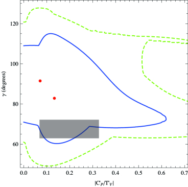
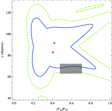
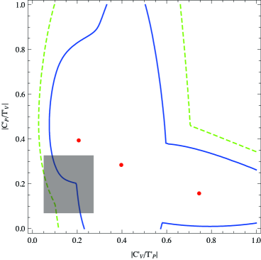
Figure 1: Fit1-a: correlation between the weak phase $\gamma$ and the ratio $|C^{\prime}_{P}/T^{\prime}_{V}|$ (left plot) or $|T^{\prime}_{P}/P^{\prime}_{P}|$ (right plot). The (red) dots correspond to the solutions listed in Table 3. The contours of $\Delta\chi^{2}=1$ and $2$ from the best solution ($\chi^{2}_{min}=0.98$) are indicated by the solid (blue) and dashed (green) curves. The shaded region is given by the 1$\sigma$ ranges of Eqs. (5) and (S0.Ex9) for comparison.

Figure 2: Fit1-b: correlation between the ratios $|C^{\prime}_{P}/T^{\prime}_{V}|$ and $|C^{\prime}_{V}/T^{\prime}_{P}|$. The (red) dots correspond to the solutions listed in Table 3. The contours of $\Delta\chi^{2}=1$ and $2$ from the best solution ($\chi^{2}_{min}=1.66$) are indicated by the solid (blue) and dashed (green) curves. The shaded region is given by the 1$\sigma$ ranges of Eqs. (5) and (S0.Ex9) for comparison.

The situation is similar in Fig. 2. Here we see the correlation between the ratios $|C^{\prime}_{P}/T^{\prime}_{V}|$ and $|C^{\prime}_{V}/T^{\prime}_{P}|$ for Fit1-b. As indicated in Table 6, the shaded region is consistent with two central values, and inconsistent with the third. However, when fit errors are included, the shaded area is included in the allowed regions (essentially completely for the “dashed region”). Once again, when the fit errors are taken into account, all solutions are in agreement with the SM.

The situation is even more striking in Fig. 3, which shows the correlation between the weak phase $\gamma$ and the ratio $|C^{\prime}_{P}/T^{\prime}_{V}|$ (left plot) or the ratios $|C^{\prime}_{P}/T^{\prime}_{V}|$ and $|C^{\prime}_{V}/T^{\prime}_{P}|$ (right plot) for Fit2-a. Taking the two plots together, one sees that all three central values ((red) dots) are inconsistent with the shaded region, that is, they all indicate NP. However, the shaded region is completely inside the “solid region.” Thus, the inclusion of the fit errors removes all inconsistencies, so that all solutions are in agreement with the SM.

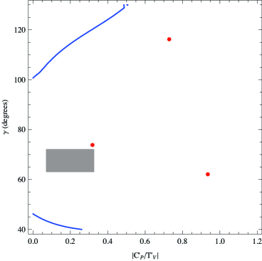
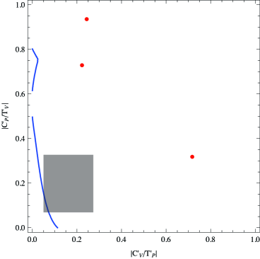
Figure 3: Fit2-a: correlation between the weak phase $\gamma$ and the ratio $|C^{\prime}_{P}/T^{\prime}_{V}|$ (left plot) or the ratios $|C^{\prime}_{P}/T^{\prime}_{V}|$ and $|C^{\prime}_{V}/T^{\prime}_{P}|$ (right plot). The (red) dots correspond to the solutions listed in Table 5. The contour of $\Delta\chi^{2}=1$ from the best solution ($\chi^{2}_{min}=0.22$) is indicated by the solid (blue) curve. The shaded region is given by the 1$\sigma$ ranges of Eqs. (5) and (S0.Ex9) for comparison.

Finally, Fig. 4 shows the correlation between the ratios $|C^{\prime}_{P}/T^{\prime}_{V}|$ and $|C^{\prime}_{V}/T^{\prime}_{P}|$ for Fit2-b. Despite the fact that the central values show some discrepancies with the shaded region, the inclusion of the fit errors removes them, so that all solutions are in agreement with the SM.

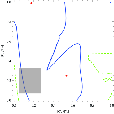
Figure 4: Fit2-b: correlation between the ratios $|C^{\prime}_{P}/T^{\prime}_{V}|$ and $|C^{\prime}_{V}/T^{\prime}_{P}|$. The (red) dots correspond to the solutions listed in Table 5. The contours of $\Delta\chi^{2}=1$ and $2$ from the best solution ($\chi^{2}_{min}=0.26$) are indicated by the solid (blue) and dashed (green) curves. The shaded region is given by the 1$\sigma$ ranges of Eqs. (5) and (S0.Ex9) for comparison.

From the figures, one sees that, when one includes the errors from the fits on the theoretical parameters, all solutions are consistent with the SM, even if the central values are not. The reason for this is that the fit errors are quite large. And this is related to the fact that the experimental errors on the $B\to K^{*}\pi$ and $B\to\rho K$ observables are also large, especially those related to the CP asymmetries. These errors are considerably larger than those in $B\to K\pi$. At present, it is not possible to clearly see if NP is present in these ${\bar{b}}\to{\bar{s}}$ $VP$ decays. Hopefully, in the future, it will be possible to increase the precision of the $B\to K^{*}\pi$ and $B\to\rho K$ measurements, so that we can further test the $\pi K$ puzzle.

In summary, we have performed fits to $B\to K^{*}\pi$ and $B\to\rho K$ decays within the standard model (SM). In particular, we have employed the relations between electroweak-penguin and tree amplitudes to couple together the two types of decay modes, which are otherwise separate. Our fits are of two types: those in which the weak phase $\gamma$ is extracted from the $B$-decay data, and those in which an independent determination of $\gamma$ [Eq. (5)] is imposed. We begin our analysis by neglecting $P^{\prime}_{uc}$. We find that the central value of $\gamma$ tends to be larger when no independent determination is imposed (Fit1-a). When Eq. (5) is taken into account, two of the solutions are consistent with the SM expectations, while the other has a somewhat large $|C^{\prime}_{V}/T^{\prime}_{P}|$ ratio (Fit1-b). Next we include $P^{\prime}_{uc}$ in the fits. Without using the external constraint on $\gamma$, all three solutions have a problem with too-large $|C^{\prime}/T^{\prime}|$ ratios. In addition, one of these gives a too-large value for $\gamma$ (Fit2-a). They could indicate the presence of new physics (NP). After imposing Eq. (5), there are two solutions. One of these still has the problem of a large $|C^{\prime}/T^{\prime}|$, while the other is improved (Fit2-b).

These problems with the theory parameters potentially show some hints of NP. However, the fits also yield large errors on these parameters. There is no serious discrepancy with the predictions of the SM when these errors are taken into account. In order to make more decisive conclusions about NP in $B\to K^{*}\pi$ and $B\to\rho K$, the uncertainties on the measurements of observables have to be reduced, particularly for the CP asymmetries. Such efforts will be paid off by shedding additional light on the $B\to\pi K$ puzzle.

Acknowledgments: C.C. would like to thank the hospitality of NCTS-Hsinchu. This work was financially supported by Grant No. NSC 97-2112-M-008-002-MY3 of Taiwan (CC) and by NSERC of Canada (DL).

References

- [1] S. Baek, C. W. Chiang and D. London, Phys. Lett. B 675, 59 (2009).
- [2] C. W. Chiang and Y. F. Zhou, JHEP 0903, 055 (2009), and references therein.
- [3] C. Isola, M. Ladisa, G. Nardulli and P. Santorelli, Phys. Rev. D 68, 114001 (2003) [arXiv:hep-ph/0307367].
- [4] Q. Chang, X. Q. Li and Y. D. Yang, JHEP 0809, 038 (2008).
- [5] M. Gronau, Phys. Rev. D 62, 014031 (2000).
- [6] W. M. Sun, Phys. Lett. B 573, 115 (2003).
- [7] C. W. Chiang, arXiv:hep-ph/0502183.
- [8] Updated results and references are tabulated periodically by the Heavy Flavor Averaging Group: http://www.slac.stanford.edu/xorg/hfag/rare.
- [9] B. Aubert et al. [BABAR Collaboration], Phys. Rev. D 71, 111101 (2005).
- [10] B. Aubert et al. [BABAR Collaboration], Phys. Rev. D 74, 051104 (2006).
- [11] B. Aubert et al. [BABAR Collaboration], arXiv:0708.2097 [hep-ex].
- [12] B. Aubert et al. [BABAR Collaboration], Phys. Rev. D 78, 052005 (2008).
- [13] B. Aubert et al. [BABAR Collaboration], Phys. Rev. D 78, 012004 (2008).
- [14] B. Aubert et al. [BABAR Collaboration], arXiv:0807.4567 [hep-ex].
- [15] P. Chang et al. [Belle Collaboration], Phys. Lett. B 599, 148 (2004).
- [16] A. Garmash et al. [Belle Collaboration], Phys. Rev. Lett. 96, 251803 (2006).
- [17] A. Garmash et al. [Belle Collaboration], Phys. Rev. D 75, 012006 (2007).
- [18] I. Adachi et al. [Belle Collaboration], Belle BELLE-CONF-0827 (2008).
- [19] J. Dalseno et al. [Belle Collaboration], arXiv:0811.3665 [hep-ex].
- [20] C. P. Jessop et al. [CLEO Collaboration], Phys. Rev. Lett. 85, 2881 (2000).
- [21] E. Eckhart et al. [CLEO Collaboration], Phys. Rev. Lett. 89, 251801 (2002).
- [22] B. I. Eisenstein et al. [CLEO Collaboration], Phys. Rev. D 68, 017101 (2003).
- [23] CKMfitter Group, J. Charles et al., Eur. Phys. J. C 41, 1 (2005).
- [24] M. Beneke and M. Neubert, Nucl. Phys. B 675, 333 (2003).
- [25] For example, see C. S. Kim, S. Oh and Y. W. Yoon, Phys. Lett. B 665, 231 (2008).