Wave breaking in the Ostrovsky–Hunter equation

Abstract

The Ostrovsky–Hunter equation governs evolution of shallow water waves on a rotating fluid in the limit of small high-frequency dispersion. Sufficient conditions for the wave breaking in the Ostrovsky–Hunter equation are found both on an infinite line and in a periodic domain. Using the method of characteristics, we also specify the blow-up rate at which the waves break. Numerical illustrations of the finite-time wave breaking are given in a periodic domain.

1 Introduction

The nonlinear evolution equation

(1.1) $$\left(u_{t}+uu_{x}-\beta u_{xxx}\right)_{x}=\gamma u,$$

with $\beta,\gamma\in\mathbb{R}$ and $u(t,x):\mathbb{R}_{+}\times\mathbb{R}\mapsto\mathbb{R}$, was derived by Ostrovsky [16] to model small-amplitude long waves in a rotating fluid of a finite depth. This equation generalizes the Korteweg–de Vries equation (that corresponds to $\gamma=0$) by the additional term induced by the Coriolis force. Mathematical properties of the Ostrovsky equation (1.1) were studied recently in many details, including the local and global well-posedness in energy space [6, 10, 22, 25], stability of solitary waves [8, 11, 12], and convergence of solutions in the limit of the Korteweg–de Vries equation [9, 12].

We shall consider the limit of no high-frequency dispersion $\beta=0$, when the evolution equation (1.1) can be written in the form

(1.2) $$\left\{\begin{array}[]{l}(u_{t}+uu_{x})_{x}=\gamma u,\quad t>0,\\ u(0,x)=u_{0}(x),\end{array}\right.$$

where $x$ is considered either on a circle or on an infinite line. In this form, the main equation (1.2) is known under different names such as the reduced Ostrovsky equation [17, 21], the Ostrovsky–Hunter equation [1], the short-wave equation [5], and the Vakhnenko equation [15, 23]. We shall use the name of the Ostrovsky–Hunter equation for convenience. We also consider $\gamma>0$ since the other case $\gamma<0$ is covered by the reflection $x\to-x$ and $u\to-u$ of the solutions for $\gamma>0$.

According to the method of characteristics, the simple-wave equation $u_{t}+uu_{x}=0$ (that corresponds to $\gamma=0$) develops wave breaking in a finite time for any initial data $u(0,x)=u_{0}(x)$ on an infinite line or in a periodic domain if $u_{0}(x)$ is continuously differentiable and there is a point $x_{0}$ such that $u_{0}^{\prime}(x_{0})<0$. More precisely, we say that the finite-time wave breaking occurs if there exists a finite time $T\in(0,\infty)$ such that

(1.3) $$\liminf_{t\uparrow T}\inf_{x}u_{x}(t,x)=-\infty,\quad\mbox{while}\quad\limsup_{t\uparrow T}\sup_{x}\left|u(t,x)\right|<\infty.$$

In view of the result for $\gamma=0$, we address the question if the low-frequency dispersion term with $\gamma>0$ in the Ostrovsky–Hunter equation (1.2) can stabilize global dynamics of the simple-wave equation $u_{t}+uu_{x}=0$.

Hunter [5] found a sufficient condition for wave breaking of the Cauchy problem (1.2) in a periodic domain and provided numerical evidences of the finite-time wave breaking for the sinusoidal initial data $u_{0}(x)$. To be precise, the main result of [5] can be formulated as follows.

Theorem 1 (Hunter, 1990).

Let $u_{0}(x)\in C^{1}(\mathbb{S})$, where $\mathbb{S}$ is a circle of unit length and define

$$\inf_{x\in\mathbb{S}}u_{0}^{\prime}(x)=-m\quad\mbox{\rm and}\quad\sup_{x\in\mathbb{S}}\left|u_{0}(x)\right|=M.$$

If $m^{3}>4M(4+m)$, a smooth solution $u(t,x)$ of the Cauchy problem (1.2) with $\gamma=1$ breaks down at a finite time $T\in(0,2m^{-1})$.

We shall study wave breaking of the Cauchy problem (1.2) in more details. First, the Cauchy problem is shown to be locally well-posed if $u_{0}\in H^{s}$, $s\geq 2$ both on an infinite line $\mathbb{R}$ and on a unit circle $\mathbb{S}$. The blow-up alternative is derived to claim that the solution $u(t,x)$ blows up in a finite time in the $H^{s}$ norm with $s\geq 2$ if and only if $\inf_{x}u_{x}(t,x)$ becomes unbounded from below. Using the integral estimates and the method of characteristics similar to analysis of the Camassa–Holmes equation in [2, 3] and the Degasperis–Processi equation in [13, 14], we find various sufficient conditions for the wave breaking, which are sharper than Theorem 1. Moreover, we also obtain the blow-up rate at which the waves break in a finite time.

We note that, unlike the Ostrovsky equation (1.1), the Ostrovsky–Hunter equation (1.2) is integrable using the inverse scattering transform method [23]. This method allows us to solve the initial-value problem (1.2) formally by working with the spectral theory for a third-order differential operator, which is similar to the Lax operator for the Hirota–Satsuma equation [19]. As a particular property of an integrable model, the Ostrovsky–Hunter equation (1.2) has a hierarchy of conserved quantities, which follows from results of [24] and [19] after exchanging densities and fluxes. This hierarchy includes the first two conserved quantities

(1.4) $$Q=\int u^{2}dx,\quad E=\int\left[\gamma(\partial_{x}^{-1}u)^{2}+\frac{1}{3}u^{3}\right]dx,$$

where the anti-derivative operator is defined by the integration of $u(t,x)$ in $x$ subject to the zero-mass constraint $\int udx=0$. Higher-order conserved quantities of the Ostrovsky–Hunter equation (1.2) involve higher-order anti-derivatives, which are defined under additional constraints on the solution $u(t,x)$. Therefore, conserved quantities of the Ostrovsky–Hunter equation are not related to the $H^{s}$-norms and hence are not so useful in the study of global well-posedness in the energy space, in a sharp contrast with very similar short-pulse and Hirota–Satsuma equations studied in [18] and [4], respectively. Our analysis does not rely, therefore, on integrability properties of the Ostrovsky–Hunter equation (1.2). We also emphasize that integrability of the nonlinear evolution equations does not prevent a finite-time blow-up, see [2, 3, 13, 14] for analysis of wave breaking in other integrable equations.

The other problem related to the subject of this paper is the existence and stability of spatially periodic and localized traveling-wave solutions $u(t,x)=\varphi(x-ct)$ with speed $c\in\mathbb{R}$. Function $\varphi(x)$ is defined by solutions of the differential equation

(1.5) $$(c-\varphi(x))\varphi^{\prime\prime}(x)=(\varphi^{\prime}(x))^{2}-\gamma\varphi(x),$$

where $x$ is considered either on a circle or on an infinite line. Bounded $2\pi$-periodic solutions $\varphi(x)$ were shown in [1] to exist for the wave speeds

$$1\leq\frac{c}{\gamma}\leq\frac{\pi^{2}}{9},$$

where $c=\gamma$ corresponds to the small-amplitude sinusoidal wave and $c=\frac{\pi^{2}}{9}\gamma$ corresponds to the large-amplitude crest wave (called the parabolic wave) which is given by the piecewise continuous quadratic polynomial in $x$

$$\varphi(x)=\frac{\gamma}{16}(3x^{2}-\pi^{2}),\quad x\in[-\pi,\pi],$$

with a discontinuous slope at the crests located at $x=\pm\pi$. Analytical and numerical approximations of the periodic wave solutions can be found in [1] and [5]. Our results on wave breaking in a periodic domain $\mathbb{S}$ do not exclude possibility of global well-posedness of the Cauchy problem for small initial data $u_{0}(x)$ and stability of periodic wave solutions satisfying (1.5). The latter problems are left, however, beyond the scopes of this paper.

No localized solutions $\varphi(x)$ were found on a real line $\mathbb{R}$, except for multi-valued loop solitons [15] and other exotic solutions [17, 21] that do not belong to $H^{s}(\mathbb{R})$ with $s\geq 2$. In Appendix A, we prove that no classical solutions $\varphi(x)\in C^{2}(\mathbb{R})$ with decay

$$\lim_{|x|\to\infty}\varphi(x)=\lim_{|x|\to\infty}\varphi^{\prime}(x)=0$$

exist. Again, global well-posedness of the Cauchy problem on an infinite line for small initial data $u_{0}(x)$ is not excluded by our results.

The paper is organized as follows. Section 2 gives a sufficient condition for the wave breaking in a periodic domain. The blow-up rate of the wave breaking is studied in Section 3 based on the method of characteristics. Similar results on an infinite line are reported in Section 4. Section 5 gives numerical evidences of wave breaking in a periodic domain. Appendix A contains results on non-existence of localized traveling-wave solutions.

2 Wave breaking in a periodic domain

Let $\gamma>0$ and $\mathbb{S}$ denote a circle of a unit length. Local well-posedness of the Cauchy problem (1.2) with initial data $u_{0}\in H^{s}(\mathbb{S})$, $s\geq 2$ can be obtained using the work of Schäfer & Wayne [20] who studied a very similar short-pulse equation

(2.1) $$\left\{\begin{array}[]{l}u_{xt}=u+(u^{3})_{xx},\quad t>0,\\ u(0,x)=u_{0}(x),\end{array}\right.$$

on an infinite line. More precisely, we have the following local well-posedness result.

Lemma 1.

Assume that $u_{0}(x)\in H^{s}(\mathbb{S})$, $s\geq 2$ and $\int_{\mathbb{S}}u_{0}(x)\,dx=0$. Then there exist a maximal time $T=T(u_{0})>0$ and a unique solution $u(t,x)$ to the Cauchy problem (1.2) such that

$$u(t,x)\in C([0,T);H^{s}(\mathbb{S}))\cap C^{1}([0,T);H^{s-1}(\mathbb{S}))$$

with the following two conserved quantities

$$\int_{\mathbb{S}}u(t,x)dx=0,\qquad t\in[0,T)$$

and

$$\int_{\mathbb{S}}u^{2}(t,x)dx=\int_{\mathbb{S}}u_{0}^{2}(x)dx,\qquad t\in[0,T).$$

Moreover, the solution depends continuously on the initial data, i.e. the mapping $u_{0}\mapsto u:\;H^{s}(\mathbb{S})\rightarrow C([0,T);H^{s}(\mathbb{S}))\cap C^{1}([0,T);H^{s-1}(\mathbb{S}))$ is continuous.

Proof.

Existence, uniqueness, and continuous dependence in $H^{s}(\mathbb{R})$, $s\geq 2$ were proven in [20] in the content of the short-pulse equation (2.1). The same method based on modified Picard’s iterations works in $H^{s}(\mathbb{S})$, so that the first part of Lemma 1 is an extension of the main theorem of [20] to a periodic domain. To prove the zero-mass constraint, we note that $u_{t}\in C([0,T);H^{1})$ and $uu_{x}\in C([0,T);H^{1})$ for the solution $u\in C([0,T);H^{s}(\mathbb{S}))\cap C^{1}([0,T);H^{s-1}(\mathbb{S}))$ with $s\geq 2$. By Sobolev’s embedding of $H^{1}(\mathbb{S})$ to $C(\mathbb{S})$, we obtain

$$\gamma\int_{\mathbb{S}}u(t,x)\,dx=\int_{\mathbb{S}}u_{tx}\,dx+\int_{\mathbb{S}}(uu_{x})_{x}\,dx=0,\quad t\in(0,T).$$

To prove conservation of the $L^{2}$-norm, we consider the balance equation

$$(u^{2})_{t}=\left(\gamma(\partial_{x}^{-1}u)^{2}-\frac{2}{3}u^{3}\right)_{x},\quad x\in\mathbb{S},\quad t\in(0,T),$$

where $\partial_{x}^{-1}u=\gamma^{-1}(u_{t}+uu_{x})\in C([0,T);H^{1}(\mathbb{S}))$, so that $\partial_{x}^{-1}u(t,x)$ is continuous on $\mathbb{S}$ for all $t\in[0,T)$. Integrating the balance equation, we obtain

$$\int_{\mathbb{S}}u^{2}(t,x)\,dx=\int_{\mathbb{S}}u_{0}^{2}(x)\,dx,\quad t\in[0,T).$$

This completes the proof of Lemma 1. ∎

Remark 1.

The assumption $\int_{\mathbb{S}}u_{0}(x)\,dx=0$ in Lemma 1 on the initial data $u_{0}$ is necessary. In fact, the zero-mass constraint on $u_{0}$ can be derived from the following estimate

$$\left|\int_{\mathbb{S}}u(t,x)\,dx-\int_{\mathbb{S}}u_{0}(x)\,dx\right|\leq\|u(t,\cdot)-u_{0}(\cdot)\|_{L^{2}(\mathbb{S})},\quad\forall t\in(0,T).$$

Note that $\int_{\mathbb{S}}u(t,x)\,dx=0,$ for all $t\in(0,T)$ and $u\in C([0,T);H^{2}(\mathbb{S})).$ Hence the above estimate implies in the limit $t\downarrow 0$ that $\int_{\mathbb{S}}u_{0}(x)dx=0$. Note that no zero-mass constraint on $u_{0}$ is necessary on an infinite line [20].

Remark 2.

The maximal time $T>0$ in Lemma 1 is independent of $s\geq 2$ in the following sense. If $u_{0}(x)\in H^{s}(\mathbb{S})\cap H^{s^{\prime}}(\mathbb{S})$ for $s,s^{\prime}\geq 2$ and $s\neq s^{\prime}$, then

$$u(t,x)\in C([0,T);H^{s}(\mathbb{S}))\cap C^{1}([0,T);H^{s-1}(\mathbb{S}))$$

and

$$u(t,x)\in C([0,T^{\prime});H^{s^{\prime}}(\mathbb{S}))\cap C^{1}([0,T^{\prime});H^{s^{\prime}-1}(\mathbb{S}))$$

with the same $T^{\prime}=T$. See Yin [26] for an adaptation of the Kato method [7] to the proof of this statement.

By using the local well-posedness result in Lemma 1 and energy estimates, one can get the following precise blow-up scenario of the solutions to the Cauchy problem (1.2).

Lemma 2.

Let $u_{0}(x)\in H^{s}(\mathbb{S})$, $s\geq 2$ and $u(t,x)$ be a solution of the Cauchy problem (1.2) in Lemma 1. The solution blows up in a finite time $T\in(0,\infty)$ in the sense of $\lim_{t\uparrow T}\|u(t,\cdot)\|_{H^{s}}=\infty$ if and only if

$$\lim_{t\uparrow T}\inf_{x\in\mathbb{S}}u_{x}(t,x)=-\infty.$$

Proof.

Assume a finite maximal existence time $T\in(0,\infty)$ and suppose there is $M>0$ such that

(2.2) $$\inf_{x\in\mathbb{S}}u_{x}(t,x)\geq-M,\quad\forall t\in[0,T).$$

Applying density arguments, we approximate initial value $u_{0}(x)\in H^{2}(\mathbb{S})$ by functions $u_{0}^{n}(x)\in H^{3}(\mathbb{S})$, $n\geq 1$, so that $\lim_{n\to\infty}u_{0}^{n}=u_{0}$. Furthermore, write $u^{n}(t,x)$ for the solution of the Cauchy problem (1.2) with initial data $u_{0}^{n}(x)\in H^{3}(\mathbb{S})$. Using the regularity result proved in Lemma 1, it follows from Sobolev’s embedding that, if $u^{n}(t,x)\in C([0,T);H^{3}(\mathbb{S}))$, then $u^{n}(t,x)$ is a twice continuously differentiable periodic function of $x$ on $\mathbb{S}$ for any $t\in[0,T)$. It is then deduced from the Ostrovsky–Hunter equation (1.2) that

$$\frac{d}{dt}\int_{\mathbb{S}}(u^{n}_{x})^{2}dx=-\int_{\mathbb{S}}u^{n}_{x}(u^{n}_{x})^{2}dx\leq M\int_{\mathbb{S}}(u^{n}_{x})^{2}dx,$$

and

$$\frac{d}{dt}\int_{\mathbb{S}}(u^{n}_{xx})^{2}dx=-5\int_{\mathbb{S}}u^{n}_{x}(u^{n}_{xx})^{2}dx\leq 5M\int_{\mathbb{S}}(u^{n}_{xx})^{2}dx,$$

where we have used the uniform bound (2.2). The Gronwall inequality then yields

$$\|u^{n}_{x}\|_{L^{2}}\leq\|(u_{0}^{n})^{\prime}\|_{L^{2}}e^{\frac{M}{2}t},\quad$$

and

$$\|u^{n}_{xx}\|_{L^{2}}\leq\|(u_{0}^{n})^{\prime\prime}\|_{L^{2}}e^{\frac{5}{2}Mt},\quad 0\leq t<T.$$

Since $\|u^{n}_{0}\|_{H^{2}}$ converges to $\|u_{0}\|_{H^{2}}$ as $n\to\infty$, we infer from the continuous dependence of the local solution $u$ on initial data $u_{0}$ that the norm in $H^{2}(\mathbb{S})$ of the solution $u$ in Lemma 1 does not blow up in the finite time $T<\infty$ and therefore either $T$ is not a maximal existence time or the bound (2.2) does not hold as $t\uparrow T$. Since $T$ is independent on $s\geq 2$ by Remark 2, the norm in $H^{s}(\mathbb{S})$ for any $s\geq 2$ of the solution in Lemma 1 blows up in a finite time $T\in(0,\infty)$ if and only if the bound (2.2) does not hold as $t\uparrow T$. ∎

The main result of this section is the following sufficient condition for the wave breaking in the Ostrovsky–Hunter equation (1.2).

Theorem 2.

Assume that $u_{0}(x)\in H^{s}(\mathbb{S})$, $s\geq 2$ and $\int_{\mathbb{S}}u_{0}(x)\,dx=0$. If $u_{0}$ satisfies either

(2.3) $$\int_{\mathbb{S}}\left(u_{0}^{\prime}(x)\right)^{3}\,dx<-\left(\frac{3\gamma}{2}\|u_{0}\|_{L^{2}}\right)^{3/2}$$

or

(2.4) $$\int_{\mathbb{S}}\left(u_{0}^{\prime}(x)\right)^{3}\,dx<0\quad\mbox{and}\quad\|u_{0}\|_{L^{2}}>\frac{3\gamma}{4},$$

then the solution $u(t,x)$ of the Cauchy problem (1.2) in Lemma 1 blows up in finite time $T\in(0,\infty)$ in the sense of Lemma 2.

Proof.

Let $T>0$ be the maximal time of existence of the solution $u(t,x)$ in Lemma 1. Then, we obtain the a priori differential estimate

$$\frac{d}{dt}\int_{\mathbb{S}}u_{x}^{3}\,dx = 3\int_{\mathbb{S}}u_{x}^{2}\left(-u_{x}^{2}-uu_{xx}+\gamma u\right)\,dx$$

$$= -2\int_{\mathbb{S}}u_{x}^{4}\,dx+3\gamma\int_{\mathbb{S}}uu_{x}^{2}\,dx$$

$$\leq -2\|u_{x}\|^{4}_{L^{4}}+3\gamma\|u\|_{L^{2}}\|u_{x}\|^{2}_{L^{4}}$$

$$= -2\left(\|u_{x}\|^{2}_{L^{4}}-\frac{3\gamma}{4}\|u_{0}\|_{L^{2}}\right)^{2}+\frac{9\gamma^{2}}{8}\|u_{0}\|_{L^{2}}^{2},$$

where we have used the Cauchy–Schwarz inequality and the $L^{2}$-norm conservation. An application of Hölder’s inequality yields

(2.5) $$\|u_{x}\|^{3}_{L^{3}}\leq\|u_{x}\|^{3}_{L^{4}}.$$

Let $V(t)=\int_{\mathbb{S}}u_{x}^{3}(t,x)\,dx$ for all $t\in[0,T)$, $Q_{0}=\|u_{0}\|_{L^{2}}$, and assume that

$$V(0)<-\left(\frac{3\gamma Q_{0}}{2}\right)^{\frac{3}{2}}<0.$$

Then, we have

$$\|u_{x}\|^{2}_{L^{4}}-\frac{3\gamma}{4}\|u_{0}\|_{L^{2}}\geq\|u_{x}\|^{2}_{L^{3}}-\frac{3\gamma}{4}\|u_{0}\|_{L^{2}}\geq|V|^{\frac{2}{3}}-\frac{3\gamma Q_{0}}{4},$$

so that the a priori differential inequality is closed at

$$\frac{dV}{dt}\leq-2\left(|V|^{\frac{2}{3}}-\frac{3\gamma Q_{0}}{4}\right)^{2}+\frac{9\gamma^{2}Q_{0}^{2}}{8},$$

where the right-hand-side is negative at $t=0$. By the continuation argument, $V(t)$ is decreasing on $[0,T)$ so that $V(t)\leq V(0)<0$. We need to prove that $T$ is finite and $\lim_{t\uparrow T}V(t)=-\infty$. Let $y=|V|^{1/3}$ and obtain that

$$\frac{dy}{dt}\geq\frac{2}{3}\left(y^{2}-\frac{3\gamma Q_{0}}{2}\right),$$

where the right-hand-side is positive at $t=0$. By the comparison principle for differential equations $y(t)\geq y^{+}(t)$ for all $t\in[0,T)$, where $y^{+}(t)$ solves the differential equation

$$\left\{\begin{array}[]{l}\dot{y}^{+}=\frac{2}{3}\left((y^{+})^{2}-\frac{3\gamma Q_{0}}{2}\right),\\ y^{+}(0)=y(0)\end{array}\right.$$

Since $y(0)>\left(\frac{3\gamma Q_{0}}{2}\right)^{\frac{1}{2}}$, there is a finite time $T^{+}\in(0,\infty)$ such that $\lim_{t\uparrow T^{+}}y^{+}(t)=+\infty$ and therefore, there is a time $T\in(0,T^{+})$ such that $\lim_{t\uparrow T^{+}}y(t)=+\infty$.

To prove the second sufficient condition (2.4), we note that since $\int_{\mathbb{S}}u(t,x)dx=0$, for each $t\in[0,T)$ there is a $\xi_{t}\in\mathbb{S}$ such that $u(t,\xi_{t})=0$. Then for any $x\in[\xi_{t},\xi_{t}+\frac{1}{2}]$, we have

$$u^{2}(t,x)=\left(\int_{\xi_{t}}^{x}u_{x}(t,x)\,dx\right)^{2}\leq(x-\xi_{t})\int^{x}_{\xi_{t}}u_{x}^{2}(t,x)\,dx\leq\frac{1}{2}\|u_{x}\|_{L^{2}}^{2}.$$

Combining it with a similar estimate on $[\xi_{t}+\frac{1}{2},\xi_{t}+1]$ thanks to periodicity of $u(t,x)$ in $x$ for all $t\in[0,T)$, we have

$$\sup_{x\in\mathbb{S}}u^{2}(t,x)\leq\frac{1}{2}\|u_{x}\|^{2}_{L^{2}}\leq\frac{1}{2}\|u_{x}\|^{2}_{L^{4}}.$$

Therefore, continuing the a priori differential inequality above, we obtain

$$\frac{d}{dt}\int_{\mathbb{S}}u_{x}^{3}\,dx \leq -2\|u_{x}\|^{4}_{L^{4}}+3\gamma\|u\|_{L^{2}}\|u_{x}\|^{2}_{L^{4}}$$

$$\leq -2\|u_{x}\|^{4}_{L^{4}}+3\gamma\|u_{0}\|_{L^{2}}^{-1}\|u\|_{L^{\infty}}^{2}\|u_{x}\|^{2}_{L^{4}}$$

$$\leq -\alpha\|u_{x}\|_{L^{4}}^{4},$$

where $\alpha=2-\frac{3\gamma}{2\|u_{0}\|_{L^{2}}}>0$ by the assumption. By the same Hölder’s inequality, we obtain

$$\frac{dV}{dt}\leq-\alpha|V|^{\frac{4}{3}}.$$

where $V(t)=\int_{\mathbb{S}}u_{x}^{3}(t,x)\,dx$ for all $t\in[0,T)$ and $V(0)<0$ is assumed. Then, by the comparison principle, $V(t)\leq V^{-}(t)$ for all $t\in[0,T)$, where $V^{-}(t)$ solves the differential equation

$$\left\{\begin{array}[]{l}\dot{V}^{-}=-\alpha(V^{-})^{\frac{4}{3}},\\ V^{-}(0)=V(0).\end{array}\right.$$

Since $V(0)<0$, there is a finite time $T^{-}\in(0,\infty)$ such that $\lim_{t\uparrow T}V^{-}(t)=-\infty$ and therefore, there is a finite time $T\in(0,T^{-})$ such that $\lim_{t\uparrow T}V(t)=-\infty$. In both cases, we have

$$\inf_{x\in\mathbb{S}}u_{x}^{3}(t,x)\leq\int_{\mathbb{S}}u_{x}^{3}\,dx\equiv V(t),$$

which implies immediately that

$$\lim_{t\uparrow T}\inf_{x\in\mathbb{S}}u_{x}(t,x)=-\infty.$$

This completes the proof of the theorem. ∎

Remark 3.

Let $\inf_{x\in\mathbb{S}}u_{0}^{\prime}(x)=-m$. The first sufficient condition (2.3) in Theorem 2 can be rewritten as

$$m^{2}>\frac{3\gamma}{2}\|u_{0}\|_{L^{2}},$$

which reminds us the sufficient condition in Theorem 1 for $\gamma=1$ given by

$$m(m^{2}-4\|u_{0}\|_{L^{\infty}})>16\|u_{0}\|_{L^{\infty}}.$$

If $\|u_{0}\|_{L^{2}}$ (and then $\|u_{0}\|_{L^{\infty}}$) is large, the slope of $u_{0}^{\prime}(x)$ has to be steep enough to lead to the wave breaking. In a contrast, the second sufficient condition (2.4) in Theorem 2 shows that any smooth initial profile with $\int_{\mathbb{S}}(u_{0}^{\prime}(x))^{3}dx<0$ and sufficiently large $\|u_{0}\|_{L^{2}}$ breaks in a finite time.

3 Blow-up rate of wave breaking

We shall investigate here the blow-up rate of the wave breaking for solutions of the Cauchy problem (1.2), which we rewrite here as

(3.1) $$\left\{\begin{array}[]{l}u_{t}+uu_{x}=\gamma\partial_{x}^{-1}u,\quad x\in\mathbb{S},\;\;t>0,\\ u(0,x)=u_{0}(x),\qquad\phantom{t}x\in\mathbb{S},\end{array}\right.$$

where $\partial_{x}^{-1}$ is the mean-zero anti-derivative in the sense of

(3.2) $$\partial_{x}^{-1}u=\int_{0}^{x}u(t,x^{\prime})dx^{\prime}-\int_{\mathbb{S}}\int_{0}^{x}u(t,x^{\prime})dx^{\prime}dx.$$

We use the method of characteristics, which is also used in a similar context by Hunter [5]. Let $T>0$ be the maximal time of existence of the solution $u(t,x)$ of the Cauchy problem (3.1) in Lemma 1 with the initial data $u_{0}\in H^{s}(\mathbb{S})$ for $s\geq 2$. For all $t\in[0,T)$ and $\xi\in\mathbb{S}$, define

$$x=X(t,\xi),\quad u(t,x)=U(t,\xi),\quad\partial_{x}^{-1}u(t,x)=G(t,\xi),$$

so that

(3.3) $$\left\{\begin{array}[]{l}\dot{X}(t)=U,\\ X(0)=\xi,\end{array}\right.\quad\left\{\begin{array}[]{l}\dot{U}(t)=\gamma G,\\ U(0)=u_{0}(\xi),\end{array}\right.$$

where dots denote derivatives with respect to time $t$ on a particular characteristics $x=X(t,\xi)$ for a fixed $\xi\in\mathbb{S}$. Applying classical results in the theory of ordinary differential equations, we obtain the following two useful results on the solutions of the initial-value problem (3.3).

Lemma 3.

Let $u_{0}(x)\in H^{s}(\mathbb{S})$, $s\geq 2$ and $T>0$ be the maximal existence time of the solution $u(t,x)$ in Lemma 1. Then there exists a unique solution $X(t,\xi)\in C^{1}([0,T)\times\mathbb{S})$ to the initial-value problem (3.3). Moreover, the map $X(t,\cdot):\mathbb{S}\mapsto\mathbb{R}$ is an increasing diffeomorphism with

$$\partial_{\xi}X(t,\xi)=\exp\left(\int_{0}^{t}u_{x}(s,X(s,\xi))ds\right)>0,\,\;\forall t\in[0,T),\;\;\forall x\in\mathbb{S}.$$

Proof.

Consider the integral equation

$$X(t,\xi)=\xi+\int_{0}^{t}u(s,X(s,\xi))ds,\quad t\in[0,T),$$

where $u(t,x)\in C([0,T);H^{s}(\mathbb{S}))\cap C^{1}([0,T);H^{s-1}(\mathbb{S}))$ for $s\geq 2$, according to Lemma 1. By the ODE theory, there exists a unique solution $X(t,\xi)\in C^{1}([0,T)\times\mathbb{S})$ of the integral equation above. Using the chain rule, we obtain

$$\partial_{\xi}\dot{X}=u_{x}(t,X(t,\xi))\partial_{\xi}X\quad\Rightarrow\quad\partial_{\xi}X(t,\xi)=\exp\left(\int_{0}^{t}u_{x}(t,X(s,\xi))ds\right),$$

so that $\partial_{\xi}X(t,\xi)>0$ for all $t\in[0,T)$ and $\xi\in\mathbb{S}$. ∎

Lemma 4.

Let $u_{0}(x)\in H^{s}(\mathbb{S})$, $s\geq 2$ and $T>0$ be the maximal existence time of the solution $u(t,x)$ in Lemma 1. Then the solution $u(t,x)$ satisfies

$$\sup_{s\in[0,t]}\|u(s,\cdot)\|_{L^{\infty}}\leq\|u_{0}\|_{L^{\infty}}+\gamma t\|u_{0}\|_{L^{2}},\quad\forall t\in[0,T).$$

Proof.

By Lemma 3, the function $x=X(t,\xi)$ is invertible in $\xi\in\mathbb{S}$ for any $t\in[0,T)$. Then, we have

$$\sup_{s\in[0,t]}\sup_{x\in\mathbb{S}}|u(s,x)|=\sup_{s\in[0,t]}\sup_{\xi\in\mathbb{S}}|U(s,\xi)|,\quad t\in[0,T).$$

Since $\partial_{x}^{-1}u(t,x)\in C([0,T);H^{s+1}(\mathbb{S}))$ is the mean-zero periodic function of $x$ for each $t\in[0,T)$, there exists a $\xi_{t}\in\mathbb{S}$ such that $\partial_{x}^{-1}u(t,\xi_{t})=0$. Then for any $x\in\mathbb{S}$ and $t\in[0,T)$, we have

$$|\partial_{x}^{-1}u(t,x)|\leq\left|\int_{\xi_{t}}^{x}u(t,x)\,dx\right|\leq\int_{\mathbb{S}}|u(t,x)|dx\leq\|u_{0}\|_{L^{2}},$$

where we use the Cauchy–Schwarz inequality and the $L^{2}$ norm conservation. Using the integral equation

$$U(t,\xi)=u_{0}(\xi)+\gamma\int_{0}^{t}G(s,\xi)ds,\quad t\in[0,T),$$

we obtain

$$\sup_{s\in[0,t]}\sup_{x\in\mathbb{S}}|u(s,x)| \leq \|u_{0}\|_{L^{\infty}}+\gamma t\sup_{s\in[0,t]}\sup_{\xi\in\mathbb{S}}|G(s,\xi)|$$

$$= \|u_{0}\|_{L^{\infty}}+\gamma t\sup_{s\in[0,t]}\sup_{x\in\mathbb{S}}\left|\partial_{x}^{-1}u(s,x)\right|$$

$$\leq \|u_{0}\|_{L^{\infty}}+\gamma t\|u_{0}\|_{L^{2}},\quad t\in[0,T),$$

and the lemma is proved. ∎

Using the method of characteristics, we obtain a sufficient condition for the wave breaking in the Cauchy problem (3.1) that is different from the sufficient conditions of Theorem 2.

Theorem 3.

Let $\varepsilon>0$ and $u_{0}(x)\in H^{s}(\mathbb{S})$, $s\geq 2$. Let $T_{1}$ be the smallest positive root of

(3.4) $$2\sqrt{\gamma}T_{1}\left(\|u_{0}\|_{L^{\infty}}+\gamma T_{1}\|u_{0}\|_{L^{2}}\right)^{\frac{1}{2}}=\log\left(1+\frac{2}{\varepsilon}\right)$$

and assume that there is a $x_{0}\in\mathbb{S}$ such that

(3.5) $$u^{\prime}_{0}(x_{0})\leq-(1+\epsilon)\sqrt{\gamma}\left(\|u_{0}\|_{L^{\infty}}+\gamma T_{1}\|u_{0}\|_{L^{2}}\right)^{\frac{1}{2}}.$$

Then the solution $u(t,x)$ in Lemma 1 blows up in a finite time $T\in(0,T_{1})$ in the sense of Lemma 2.

Proof.

Define $V(t,\xi)=u_{x}(t,X(t,\xi))$. By Lemmas 1 and 3, $V(t,\xi)$ is absolutely continuous on $[0,T)\times\mathbb{S}$ and almost everywhere differentiable on $(0,T)\times\mathbb{S}$, so that

$$\dot{V}=\left(u_{tx}+uu_{xx}\right)\biggr{|}_{x=X(t,\xi)}=\left(\gamma u-u_{x}^{2}\right)\biggr{|}_{x=X(t,\xi)}=-V^{2}+\gamma U,\quad{\rm a.e.}\quad\xi\in\mathbb{S},\quad t\in(0,T).$$

By Lemma 4, we obtain the apriori differential estimate

(3.6) $$\dot{V}\leq-V^{2}+\gamma\left(\|u_{0}\|_{L^{\infty}}+\gamma t\|u_{0}\|_{L^{2}}\right),\quad{\rm a.e.}\quad\xi\in\mathbb{S},\quad t\in(0,T).$$

Since $u_{0}^{\prime}(x)$ is a continuous, mean-zero, periodic function of $x$ on $\mathbb{S}$ and assumption (3.5) is satisfied for fixed $\varepsilon>0$, there exists $\tilde{x}_{0}$ such that

$$V(0,\tilde{x}_{0})=-(1+\varepsilon)h(T_{1}),$$

where

$$h(T_{1})=\sqrt{\gamma}\left(\|u_{0}\|_{L^{\infty}}+\gamma T_{1}\|u_{0}\|_{L^{2}}\right)^{\frac{1}{2}}.$$

Thanks to the apriori estimate (3.6), $V(t):=V(t,\tilde{x}_{0})$ satisfies

(3.7) $$\left\{\begin{array}[]{l}\dot{V}(t)\leq-V^{2}(t)+h^{2}(T_{1}),\quad{\rm a.e.}\quad t\in[0,T_{1}]\cap(0,T),\\ V(0)=-(1+\varepsilon)h(T_{1}).\end{array}\right.$$

By the comparison principle for ODEs, we have

$$V(t)\leq V_{+}(t)<0,\quad t\in[0,T_{1}]\cap[0,T),$$

where $V_{+}(t)$ solves the equation

(3.8) $$\left\{\begin{array}[]{l}\dot{V}_{+}(t)=-V_{+}^{2}(t)+h^{2}(T_{1}),\quad t\in[0,T_{1}),\\ V_{+}(0)=V(0).\end{array}\right.$$

Equation (3.8) admits an implicit solution

$$\frac{V_{+}(t)+h(T_{1})}{V_{+}(t)-h(T_{1})}=\frac{V(0)+h(T_{1})}{V(0)-h(T_{1})}e^{2h(T_{1})t},\quad t\in[0,T_{1}).$$

If $T_{1}$ is the smallest positive root of (3.4), then

$$\frac{V_{+}(t)+h(T_{1})}{V_{+}(t)-h(T_{1})}=\frac{\varepsilon}{2+\varepsilon}e^{2h(T_{1})t}\uparrow 1,\quad\mbox{\rm as}\quad t\uparrow T_{1},$$

so that $\lim_{t\uparrow T_{1}}V_{+}(t)=-\infty$. Therefore, there is $T\in(0,T_{1})$ such that $\displaystyle\lim_{t\uparrow T}V(t)=-\infty$. ∎

Remark 4.

Note that if $\varepsilon\to\infty$ and the assumption of Theorem 3 still holds, then $T\to 0$. This means that the steeper the slope of the initial data $u_{0}(x)$ is, the quicker the solution $u(t,x)$ blows up.

Remark 5.

Since $\|u(t,\cdot)\|_{L^{\infty}}$ remains bounded on $[0,T)$ thanks to Lemma 4, the blow-up of Theorem 3 corresponds to criterion (1.3) of the wave breaking in the Ostrovsky–Hunter equation (1.2).

By Theorem 3, we have the following two corollaries.

Corollary 1.

Assume that $u_{0}(x)\in H^{s}(\mathbb{S})$, $s\geq 2$ is even and non-constant. Then for sufficiently large $n$, the corresponding solution $u(t,x)$ to the Cauchy problem (3.1) with initial data $u_{0}(nx)$ blows up in finite time.

Proof.

Take $x_{0}\in\mathbb{S}$ such that $u^{\prime}_{0}(x_{0})=\inf_{x\in\mathbb{S}}u^{\prime}_{0}(x)$. Since $u_{0}\in C^{1}(\mathbb{S})$ is even and periodic, it follows that $u^{\prime}_{0}(x_{0})\leq 0$ and $\sup_{x\in\mathbb{S}}u^{\prime}_{0}(x)=-u_{0}^{\prime}(x_{0})\geq 0$. Thus, we deduce that

$$\left(\inf_{x\in\mathbb{S}}u^{\prime}_{0}(x)\right)^{2}=\left(\sup_{x\in\mathbb{S}}u^{\prime}_{0}(x)\right)^{2}>\int_{\mathbb{S}}(u^{\prime}_{0}(x))^{2}dx.$$

Let $\tilde{u}_{0}(x)=u_{0}(nx)$ for a positive integer $n$. Thanks to $1$-periodicity of $u_{0}(x)$, we have $\|\tilde{u}^{\prime}_{0}\|_{L^{2}}=n\|u^{\prime}_{0}\|_{L^{2}}$, $\|\tilde{u}_{0}\|_{L^{2}}=\|u_{0}\|_{L^{2}}$, and $\|\tilde{u}_{0}\|_{L^{\infty}}=\|u_{0}\|_{L^{\infty}}$. From the above inequality, we see that the assumption of Theorem 3 for any $\varepsilon>0$ is satisfied by the initial data $\tilde{u}_{0}(x)=u_{0}(nx)$ provided $n$ is large enough. ∎

Corollary 2.

Assume that $u_{0}(x)\in H^{s}(\mathbb{S})$, $s\geq 2$ and $|\inf_{x\in\mathbb{S}}u^{\prime}_{0}(x)|\geq|\sup_{x\in\mathbb{S}}u^{\prime}_{0}(x)|>0$. Then for sufficiently large $n$, the corresponding solution $u(t,x)$ to the Cauchy problem (3.1) with initial data $u_{0}(nx)$ blows up in finite time.

Proof.

The assumption and the mean value theorem imply that there is a point $x_{0}\in\mathbb{S}$ such that

$$\left(\inf_{x\in\mathbb{S}}u^{\prime}_{0}(x)\right)^{2}\geq\left(\sup_{x\in\mathbb{S}}u^{\prime}_{0}(x)\right)^{2}>(u^{\prime}_{0}(x_{0}))^{2}\geq\int_{\mathbb{S}}(u^{\prime}_{0}(x))^{2}dx.$$

Thus, we can obtain the desired result in view of the proof of Corollary 1. ∎

Our final result specifies the rate at which the wave breaks in the Cauchy problem (3.1). We use again the fact that the blow-up time $T$ is independent of $s\geq 2$ for the solution $u(t,x)$ in Lemma 1, so that the initial data $u_{0}(x)$ can be considered in $H^{3}(\mathbb{S})$.

Theorem 4.

Let $u_{0}(x)\in H^{3}(\mathbb{S})$ and $T\in(0,\infty)$ be the finite blow-up time of the solution $u(t,x)$ in Lemma 1. Then we have

(3.9) $$\lim_{t\uparrow T}\left((T-t)\inf_{x\in\mathbb{S}}u_{x}(t,x)\right)=-1$$

and

(3.10) $$\lim_{t\uparrow T}\left((T-t)\sup_{x\in\mathbb{S}}u_{x}(t,x)\right)=0.$$

Proof.

Let $m(t):=\inf_{x\in\mathbb{S}}u_{x}(t,x)$. By the assumption of $T<\infty$ and Lemma 2, we have $\lim_{t\uparrow T}m(t)=-\infty$. By Theorem 2.1 in Constantin & Escher [3], for every $t\in[0,T)$, there exists at least one point $\xi(t)\in\mathbb{S}$ such that $m(t):=u_{x}(t,\xi(t))$ and $u_{xx}(t,\xi(t))=0$. Moreover, $m(t)$ (and $\xi(t)$) is absolutely continuous on $[0,T)$, almost everywhere differentiable on $(0,T)$, and satisfies

(3.11) $$\frac{d}{dt}m(t)=u_{tx}(t,\xi(t))=-m^{2}(t)+\gamma u(t,\xi(t))\quad{\rm a.e.}\quad t\in(0,T).$$

Set $K(T)=\gamma\left(\|u_{0}\|_{L^{\infty}}+\gamma T\|u_{0}\|_{L^{2}}\right)$. By Lemma 4, we obtain

(3.12) $$-m^{2}(t)-K(T)\leq\frac{d}{dt}m(t)\leq-m^{2}(t)+K(T)\quad{\rm a.e.}\quad t\in(0,T).$$

Let us now choose $\varepsilon\in(0,1)$. Since $\lim_{t\uparrow T}m(t)=-\infty$, one can find $t_{0}\in[0,T)$ such that

$$m(t_{0})<-\sqrt{K(T)+\frac{K(T)}{\varepsilon}}.$$

By the continuation of solutions of (3.12) and the absolute continuity of $m(t)$, it follows that $m$ is decreasing on $[t_{0},T)$ so that

$$m(t)\leq m(t_{0})<-\sqrt{K(T)+\frac{K(T)}{\varepsilon}}<-\sqrt{\frac{K(T)}{\varepsilon}},\quad t\in[t_{0},T)$$

and

$$1-\varepsilon\leq\frac{d}{dt}\left(\frac{1}{m(t)}\right)\leq 1+\varepsilon.$$

Integrating the above relation on $(t,T)$ with $t\in[t_{0},T)$ and noticing that $\lim_{t\uparrow T}m(t)=-\infty$, we deduce that

$$(1-\varepsilon)(T-t)\leq-\frac{1}{m(t)}\leq(1+\varepsilon)(T-t).$$

Since $\varepsilon\in(0,1)$ is arbitrary, in view of the definition of $m(t)$, the above inequality in the limit $\varepsilon\downarrow 0$ implies the desired result (3.9).

Now let $M(t):=\sup_{x\in\mathbb{S}}u_{x}(t,x)$. By the same Theorem 2.1 in Constantin & Escher [3], for every $t\in[0,T)$, there exists at least one point $\eta(t)\in\mathbb{S}$ such that $M(t)=u_{x}(t,\eta(t))$ and $u_{xx}(t,\eta(t))=0$. Repeating the same arguments, we have

$$\frac{d}{dt}M(t)=-M^{2}(t)+\gamma u(t,\eta(t))\leq\gamma\left(\|u_{0}\|_{L^{\infty}}+\gamma t\|u_{0}\|_{L^{2}}\right),\quad\mbox{for all}\quad t\in(0,T),$$

so that

(3.13) $$M(t)\leq\sup_{x\in\mathbb{S}}u_{0}^{\prime}(x)+\gamma\left(T\|u_{0}\|_{L^{\infty}}+\frac{\gamma T^{2}}{2}\|u_{0}\|_{L^{2}}\right)<+\infty.$$

Since $u(t,x)$ is periodic on $\mathbb{S}$ for all $t\in[0,T)$ and belong to $C([0,T);H^{3}(\mathbb{S}))$, there exists $\xi_{0}(t)\in\mathbb{S}$ for every $t\in[0,T)$ such that $u_{x}(t,\xi_{0}(t))=0$. Therefore, $M(t)\geq u_{x}(t,\xi_{0}(t))=0$ for all $t\in[0,T)$, so that bound (3.13) yields the desired result (3.10). This completes the proof of the theorem. ∎

4 Wave breaking on an infinite line

To extend our results on wave breaking in the Ostrovsky–Hunter equation (1.2) from a circle $\mathbb{S}$ to an infinite line $\mathbb{R}$, we are going to use an additional conserved quantity of the Ostrovsky–Hunter equation. Consider the Cauchy problem in the form

(4.1) $$\left\{\begin{array}[]{l}u_{t}+uu_{x}=\gamma\partial_{x}^{-1}u,\quad x\in\mathbb{R},\;\;t>0,\\ u(0,x)=u_{0}(x),\qquad\phantom{t}x\in\mathbb{R},\end{array}\right.$$

where $\gamma>0$ and $\partial_{x}^{-1}u=\int_{-\infty}^{x}u(t,x^{\prime})dx^{\prime}$. To control $\partial_{x}^{-1}u$, we define $\|u\|_{\dot{H}^{-1}}:=\|\partial_{x}^{-1}u\|_{L^{2}}$. The local well-posedness result is given by the following lemma.

Lemma 5.

Assume that $u_{0}(x)\in H^{s}(\mathbb{R})\cap\dot{H}^{-1}(\mathbb{R})$, $s\geq 2$. Then there exist a maximal time $T=T(u_{0})>0$ and a unique solution $u(t,x)$ to the Cauchy problem (4.1) such that

$$u(t,x)\in C([0,T);H^{s}(\mathbb{R})\cap\dot{H}^{-1}(\mathbb{R}))\cap C^{1}([0,T);H^{s-1}(\mathbb{R}))$$

with the following three conserved quantities

(4.2) $$\int_{\mathbb{R}}u(t,x)dx=0,\quad t\in[0,T),$$

(4.3) $$Q=\int_{\mathbb{R}}u^{2}(t,x)dx=\int_{\mathbb{R}}u_{0}^{2}(x)dx,\quad t\in[0,T),$$

and

(4.4) $$E=\int_{\mathbb{R}}\left[\gamma(\partial_{x}^{-1}u)^{2}+\frac{1}{3}u^{3}\right]dx=\int_{\mathbb{R}}\left[\gamma(\partial_{x}^{-1}u_{0})^{2}+\frac{1}{3}u_{0}^{3}\right]dx,\quad t\in[0,T).$$

Moreover, the solution depends continuously on the initial data, i.e. the mapping $u_{0}\mapsto u:\;H^{s}(\mathbb{R})\rightarrow C([0,T);H^{s}(\mathbb{R})\cap\dot{H}^{-1}(\mathbb{R}))\cap C^{1}([0,T);H^{s-1}(\mathbb{R}))$ is continuous.

Proof.

If $u_{0}(x)\in H^{s}(\mathbb{R})\cap\dot{H}^{-1}(\mathbb{R})$, then $\partial_{x}^{-1}u_{0}(x)\in H^{3}(\mathbb{R})$, so that $\int_{\mathbb{R}}u_{0}(x)dx=0$. By the main theorem in [20] in the context of the short-pulse equation (2.1), existence, uniqueness and continuous dependence of the solution $u(t,x)\in C([0,T);H^{s}(\mathbb{R}))\cap C^{1}([0,T);H^{s-1}(\mathbb{R}))$ is proved, so that

$$\gamma\partial_{x}^{-1}u(t,x)=u_{t}(t,x)+u(t,x)u_{x}(t,x)\in C((0,T);H^{s-1}(\mathbb{R})).$$

Therefore, $u(t,x)\in C([0,T);H^{s}(\mathbb{R})\cap\dot{H}^{-1}(\mathbb{R}))$ in view of continuity of $\|u\|_{\dot{H}^{-1}}$ as $t\downarrow 0$. Because $f\in H^{1}(\mathbb{R})$ implies $\lim_{|x|\to\infty}f(x)=0$, the zero-mass constraint (4.2) holds. Let us define

$$\gamma\partial_{x}^{-2}u(t,x)=\left(\partial_{x}^{-1}u(t,x)\right)_{t}+\frac{1}{2}u^{2}(t,x).$$

By uniqueness of the strong solution $u(t,x)$ satisfying the constraint (4.2) on $[0,T)$, we obtain

$$\lim_{|x|\to\infty}\partial_{x}^{-2}u(t,x)=0,\quad\forall t\in[0,T).$$

Using balance equations for the densities of $Q$ and $E$, we write

$$(u^{2})_{t} = \left(\gamma(\partial_{x}^{-1}u)^{2}-\frac{2}{3}u^{3}\right)_{x},\quad x\in\mathbb{R},\;t\in(0,T),$$

$$\left[\gamma(\partial_{x}^{-1}u)^{2}+\frac{1}{3}u^{3}\right]_{t} = \left[\gamma^{2}(\partial_{x}^{-2}u)^{2}-\frac{1}{4}u^{4}\right]_{x},\quad x\in\mathbb{R},\;t\in(0,T).$$

Integrating the balance equation in $x$ on $\mathbb{R}$ for any $t\in(0,T)$, we obtain conservation of $Q$ and $E$. Their initial values as $t\downarrow 0$ are computed from the initial condition $u_{0}(x)$ thanks to the fact that $u_{0}(x)\in H^{s}(\mathbb{R})\cap\dot{H}^{-1}(\mathbb{R})$. ∎

The blow-up alternative in Lemma 2 holds on an infinite line thanks to Sobolev’s embedding $H^{3}(\mathbb{R})$ into $C^{2}(\mathbb{R})$ and the density arguments. Since the application (2.5) of the Hölder inequality is not valid on $\mathbb{R}$, Theorem 2 can not be extended on an infinite line. However, we can still use the method of characteristics and extend Theorems 3 and 4 from $\mathbb{S}$ to $\mathbb{R}$.

For all $t\in[0,T)$ and $\xi\in\mathbb{R}$, we define

$$x=X(t,\xi),\quad u(t,x)=U(t,\xi),\quad\partial_{x}^{-1}u(t,x)=G(t,\xi),$$

so that the same system (3.3) is considered. Lemma 3 holds on $\mathbb{R}$, while Lemma 4 is replaced with the following lemma.

Lemma 6.

Let $u_{0}(x)\in H^{s}(\mathbb{R})\cap\dot{H}^{-1}(\mathbb{R})$, $s\geq 2$ and $T>0$ be the maximal existence time of the solution $u(t,x)$ in Lemma 5. The solution $u(t,x)$ satisfies

$$\sup_{s\in[0,t]}\|u(s,\cdot)\|_{L^{\infty}}\leq\|u_{0}\|_{L^{\infty}}+Ct+\frac{\gamma Q}{6}t^{2},\quad t\in[0,T),$$

where

$$C=\frac{\sqrt{\gamma}}{\sqrt{2}}\left(E+\gamma Q+\frac{1}{3}Q\|u_{0}\|_{L^{\infty}}\right)^{\frac{1}{2}}.$$

Proof.

From conserved quantities (4.3) and (4.4), we obtain

$$\|\partial_{x}^{-1}u(t,\cdot)\|^{2}_{H^{1}}=\|u(t,\cdot)\|^{2}_{L^{2}}+\|\partial_{x}^{-1}u(t,\cdot)\|^{2}_{L^{2}} = Q+\frac{1}{\gamma}\left(E-\frac{1}{3}\int_{\mathbb{R}}u^{3}(t,x)dx\right)$$

$$\leq Q+\frac{1}{3\gamma}\left(3E+Q\|u(t,\cdot)\|_{L^{\infty}}\right).$$

Let $S(t):=\sup_{s\in[0,t]}\|u(s,\cdot)\|_{L^{\infty}}$. Thanks to Sobolev’s embedding of $H^{1}$ into $L^{\infty}$, we have

$$S(t) \leq \|u_{0}\|_{L^{\infty}}+\gamma t\sup_{s\in[0,t]}\|\partial_{x}^{-1}u(s,\cdot)\|_{L^{\infty}}$$

$$\leq \|u_{0}\|_{L^{\infty}}+\gamma t\left(\frac{Q}{2}+\frac{1}{6\gamma}\left(3E+QS(t)\right)\right)^{\frac{1}{2}},$$

from which the bound on $S(t)$ is proved after algebraic manipulations. ∎

Theorem 3 is extended to the infinite line in the following theorem.

Theorem 5.

Let $\varepsilon>0$ and $u_{0}(x)\in H^{s}(\mathbb{R})\cap\dot{H}^{-1}(\mathbb{R})$, $s\geq 2$. Let $T_{1}$ be the smallest positive root of the equation

$$2\sqrt{\gamma}T_{1}\left(\|u_{0}\|_{L^{\infty}}+CT_{1}+\frac{\gamma Q}{6}T_{1}^{2}\right)^{\frac{1}{2}}=\log\left(1+\frac{2}{\varepsilon}\right)$$

and assume that there is a $x_{0}\in\mathbb{S}$ such that

$$u^{\prime}_{0}(x_{0})\leq-(1+\epsilon)\sqrt{\gamma}\left(\|u_{0}\|_{L^{\infty}}+CT_{1}+\frac{\gamma Q}{6}T_{1}^{2}\right)^{\frac{1}{2}},$$

where $C$ is defined in Lemma 6. Then the solution $u(t,x)$ in Lemma 5 blows up in a finite time $T\in(0,T_{1})$.

Proof.

The proof is similar to that of Theorem 3. ∎

Finally, Theorem 4 remains valid on an infinite line since the proof does not depend on the definition of $K(T)$.

5 Numerical evidence of wave breaking

We consider the Cauchy problem (3.1) on $\mathbb{S}$ for $\gamma=1$ and the initial data

(5.1) $$u_{0}(x)=a\cos(2\pi x)+b\sin(4\pi x),$$

where $(a,b)$ are parameters. Using elementary calculus, we compute

$$\int_{\mathbb{S}}(u_{0}^{\prime}(x))^{3}dx=-12\pi^{3}a^{2}b,\quad\int_{\mathbb{S}}u_{0}^{2}(x)dx=\frac{1}{2}(a^{2}+b^{2})$$

and

$$m = -\inf_{x\in\mathbb{S}}u_{0}^{\prime}(x)=2\pi(a+2b),$$

$$M = \sup_{x\in\mathbb{S}}|u_{0}(x)|=\frac{1}{4}\left(3a+\sqrt{a^{2}+32b^{2}}\right)\sqrt{1-\left(\frac{-a+\sqrt{a^{2}+32b^{2}}}{8b}\right)^{2}}.$$

Figure 1 compares the theoretical estimates of the wave breaking regions on the quarter-plane $(a,b)\in\mathbb{R}_{+}^{2}$. According to Theorem 1, the blow-up occurs under the condition $m^{3}>4M(4+m)$. The lower bound of the domain, where $m^{3}>4M(4+m)$, is shown by the blue line on Figure 1. According to Theorem 2, two criteria (2.3) and (2.4) exist. The lower bound of the domain, where the first criterion (2.3) is met, is shown on Figure 1 by the green curve. The domain of the second criterion (2.4) is, however, beyond the scale of Figure 1. Indeed, the latter domain corresponds to the quarter circle on $(a,b)$-plane with the radius $\frac{3}{2\sqrt{2}}\approx 1.06$. Finally, the lower bound of the domain given by the criterion of Theorem 3 is shown on Figure 1 by the red line. We can see from the figure that the latter criterion (2.3) is the sharpest one with the largest wave breaking region shown by shaded area on Figure 1.

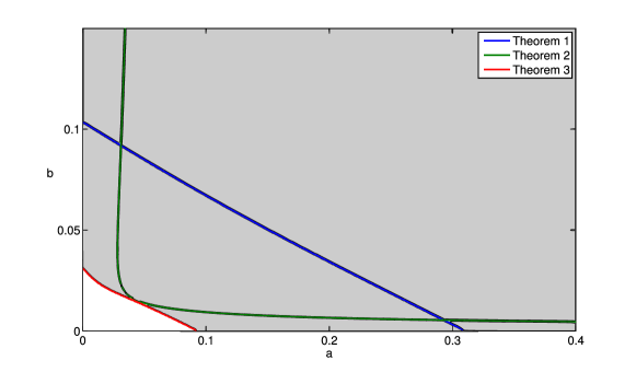
Figure 1: Lower bounds of the domains for the wave breaking conditions of Theorems 1, 2, and 3. Shaded area shows where the wave breaking condition of Theorem 3 is satisfied.

Numerical simulations of the Ostrovsky-Hunter equation (1.2) for initial data (5.1) are performed with the pseudo–spectral method for $N=4096$ Fourier harmonics with the time step of $dt=0.001$. Figures 2,3, and 4 show two dynamical evolutions for three cases $b=0$, $a=2b$, and $a=0$. In all cases, no wave breaking occur for sufficiently small values of $(a,b)$ (far below the lower bound on Figure 1) but the wave breaking does occur if the values of $(a,b)$ are selected to be larger (still below the lower bound on Figure 1). Thus, we conclude that none of the wave breaking criteria is sharp.

Right panels of Figures 2,3, and 4 show the behavior of $\inf_{x\in\mathbb{S}}u_{x}(t,x)$ versus $t$. When the wave breaking occurs (bottom panels of each figure), we compute the linear regression $B+Ct$ of $-(\inf_{x\in\mathbb{S}}u_{x}(t,x))^{-1}$, where $(B,C)$ are constants. According to Theorem 4, $B\approx T$ and $C\approx-1$ near the singularity, so that $B$ can be taken as an approximation for the blow-up time $T$ and $|C+1|$ can be taken as an estimate for the error of the linear regression. The numerical values on Figures 2,3, and 4 show that $C$ is close to $-1$ by the errors in $1\%$, $4\%$, and $6\%$, respectively.

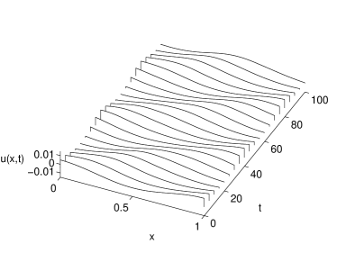
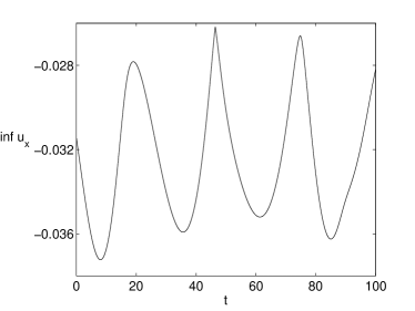
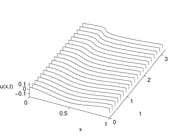
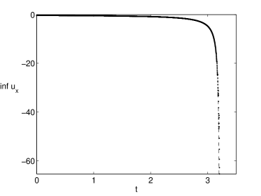
Figure 2: Solution surface $u(t,x)$ (left) and $\inf_{x\in\mathbb{S}}u_{x}(t,x)$ versus $t$ (right) for two simulations with $a=0.005$, $b=0$ (top) and $a=0.05$, $b=0$ (bottom). The dashed curve on the bottom right panel shows the least squares fit $-1/(B+Ct)$ with $C\approx-1.009$ and $B\approx 3.213$.

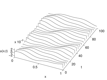
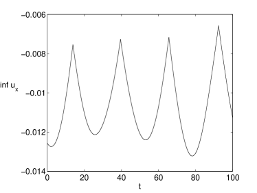
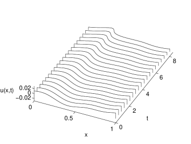
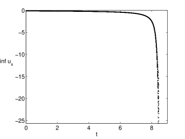
Figure 3: The same as Figure 2 but for $a=0.001$, $b=0.0005$ (top) and $a=0.01$, $b=0.005$ (bottom). The least squares fit is computed with $C\approx-1.042$ and $B\approx 8.442$.

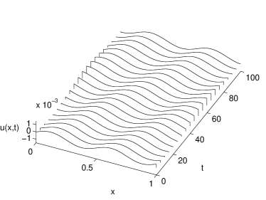
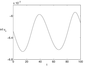
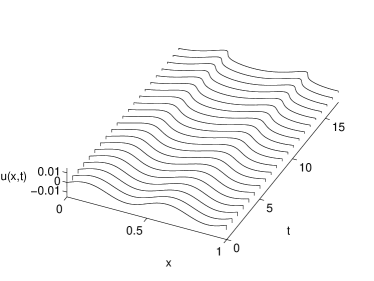
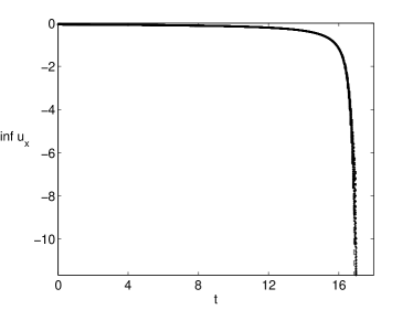
Figure 4: The same as Figure 2 but for $a=0$, $b=0.0005$ (top) and $a=0$, $b=0.005$ (bottom). The least squares fit is computed with $C\approx-1.060$ and $B\approx 16.964$.

Finally, Figure 5 shows the blow-up time $T$ estimated by the above technique versus parameters $a$ for $b=0$ and parameter $b$ for $a=0$. We can clearly see that the wave breaking holds for $(a,b)$ in the shaded area of Figure 1. The blow-up time $T$ becomes smaller for larger values of $(a,b)$.

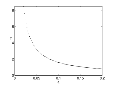
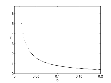
Figure 5: Estimates of the blow-up time $T$ versus $a$ for $b=0$ (left) and $b$ for $a=0$ (right).

Appendix A Appendix A:
Nonexistence of localized traveling-wave solutions

Consider the differential equation

(A.1) $$(c-\varphi(x))\varphi^{\prime\prime}(x)=(\varphi^{\prime}(x))^{2}-\gamma\varphi(x),\quad x\in\mathbb{R}$$

for traveling-wave solutions $u(t,x)=\varphi(x-ct)$ of the Ostrovsky–Hunter equation (1.2), where $c\in\mathbb{R}$ is the wave speed.

Theorem 6.

There are no nontrivial solutions of (A.1) with $c\in\mathbb{R}$ such that $\varphi\in C^{2}(\mathbb{R})$ and $\lim_{|x|\to\infty}\varphi(x)=\lim_{|x|\to\infty}\varphi^{\prime}(x)=0$.

Proof.

Arguing by contradiction, we assume the existence of $\varphi\in C^{2}(\mathbb{R})$ with $\lim_{|x|\to\infty}\varphi(x)=\lim_{|x|\to\infty}\varphi^{\prime}(x)=0$ as a solution of (A.1). Let $v(x)$ be defined by

(A.2) $$-c\varphi+\frac{1}{2}\varphi^{2}=\gamma v,$$

so that $\varphi(x)=v^{\prime\prime}(x)$. Multiplying (A.2) by $\varphi^{\prime}(x)$ and taking integral over the interval $(-\infty,\,x)$ yields

(A.3) $$-\frac{c}{2}\varphi^{2}+\frac{1}{6}\varphi^{3}+\frac{\gamma}{2}(v^{\prime})^{2}-\gamma\varphi v=0.$$

By equation (A.1), we have $\int_{\mathbb{R}}\varphi(x)\,dx=0$. Since $\varphi\in C^{2}(\mathbb{R})$, there exists a smallest zero point $\xi_{1}\in\mathbb{R}$ for $\varphi(x)$ in the sense of $\varphi(\xi_{1})=0$ and $\varphi(x)\neq 0$ for $x\in(-\infty,\,\xi_{1})$. On the other hand, it is deduced from (A.3) that $v^{\prime}(\xi_{1})=0$ and $\lim_{x\to-\infty}v^{\prime}(x)=0$. By Rolle’s theorem, there exists a point $\xi_{2}\in(-\infty,\,\xi_{1})$ such that $\varphi(\xi_{2})=v^{\prime\prime}(\xi_{2})=0$, which contradicts the assumption on the smallest $\xi_{1}$ with $\varphi(\xi_{1})=0.$ This completes the proof of the theorem. ∎

References

- [1] J. Boyd, Ostrovsky and Hunter’s generic wave equation for weakly dispersive waves: matched asymptotic and pseudospectral study of the paraboloidal travelling waves (corner and near-corner waves), Euro. Jnl. of Appl. Math. 16, 65–81 (2005).
- [2] A. Constantin, J. Escher, Well-posedness, global existence, and blowup phenomenon for a periodic quasi-linear hyperbolic equation, Comm. Pure Appl. Math. 51, 475–504 (1998).
- [3] A. Constantin and J. Escher, Wave breaking for nonlinear nonlocal shallow water equations, Acta Mathematica 181, 229–243 (1998).
- [4] R. Iorio and D. Pilod, “Well-posedness for Hirota–Satsuma equation”, Diff. Integr. Eqs. 21, 1177–1192 (2008).
- [5] J. Hunter, Numerical solutions of some nonlinear dispersive wave equations, Lectures in Appl. Math. 26, 301–316 (1990).
- [6] G. Gui and Y. Liu, “On the Cauchy problem for the Ostrovsky equation with positive dispersion”, Comm. Part. Diff. Eqs. 32, 1895–1916 (2007).
- [7] T. Kato, “On the Korteweg–de Vries equation”, Manuscripta Math. 28, 89–99 (1979).
- [8] S. Levandosky and Y. Liu, “Stability of solitary waves of a generalized Ostrovsky equation”, SIAM J. Math. Anal. 38, 985–1011 (2006)
- [9] S. Levandosky and Y. Liu, “Stability and weak rotation limit of solitary waves of the Ostrovsky equation”, Discr. Cont. Dyn. Syst. B 7, 793–806 (2007).
- [10] F. Linares and A. Milanes, “Local and global well-posedness for the Ostrovsky equation”, J. Diff. Eqs. 222, 325–340 (2006).
- [11] Y. Liu, “On the stability of solitary waves for the Ostrovsky equation”, Quart. Appl. Math. 65, 571–589 (2007).
- [12] Y. Liu and V. Varlamov, “Stability of solitary waves and weak rotation limit for the Ostrovsky equation”, J. Diff. Eqs. 203, 159183 (2004).
- [13] Y. Liu and Z.Y. Yin, “Global existence and blow-up phenomena for the Degasperis–Procesi equation”, Comm. Math. Phys. 267, 801–820 (2006).
- [14] Y. Liu and Z.Y. Yin, “On the blow-up phenomena for the Degasperis–Procesi equation”, Inter. Math. Res. Not., no.23, 117, 22 pp. (2007).
- [15] A.J. Morrison, E.J. Parkes, and V.O. Vakhnenko, “The loop soliton solutions of the Vakhnenko equation”, Nonlinearity 12, 1427–1437 (1999).
- [16] L.A. Ostrovsky, “Nonlinear internal waves in a rotating ocean”, Okeanologia 18, 181–191 (1978).
- [17] E.J. Parkes, “Explicit solutions of the reduced Ostrovsky equation”, Chaos, Solitons, and Fractals 31, 602–610 (2007).
- [18] D. Pelinovsky, A. Sakovich, Global well-posedness of the short-pulse and sine–Gordon equations in energy space, arXiv: 0809.5052 (2008).
- [19] J. Satsuma and D.J. Kaup “A Bäcklund transformation for a higher-order Korteweg–de Vries equation”, J. Phys. Soc. Japan 43, 692–697 (1977).
- [20] T. Schäfer and C. E. Wayne, “Propagation of ultra-short optical pulses in cubic nonlinear media”, Physica D 196, 90–105 (2004).
- [21] Y.A. Stepanyants, “On stationary solutions of the reduced Ostrovsky equation: periodic waves, compactons and compound solitons”, Chaos, Solitons, and Fractals 28, 193–204 (2006).
- [22] K. Tsugawa, “Well-posedness and weak rotation limit for the Ostrovsky equation”, preprint.
- [23] V.O. Vakhnenko and E.J. Parkes, “The calculation of multi-soliton solutions of the Vakhnenko equation by the inverse scattering method”, Chaos, Solitons and Fractals 13, 1819–1826 (2002).
- [24] V.O. Vakhnenko, E.J. Parkes, and A.J. Morrison, “A Bäcklund transformation and the inverse scattering transform method for the generalised Vakhnenko equation’, Chaos, Solitons and Fractals 17, 683–692 (2003).
- [25] V. Varlamov and Y. Liu, “Cauchy problem for the Ostrovsky equation”, Discr. Cont. Dyn. Syst. 10, 731–753 (2004).
- [26] Z.Y. Yin, “On the Cauchy problem for an integrable equation with peakon solutions”, Illinois J. Math. 47, 649–666 (2003).