Stability Variances: A filter Approach.

Abstract

We analyze the Allan Variance estimator as the combination of Discrete-Time linear filters. We apply this analysis to the different variants of the Allan Variance: the Overlapping Allan Variance, the Modified Allan variance, the Hadamard Variance and the Overlapping Hadamard variance. Based on this analysis we present a new method to compute a new estimator of the Allan Variance and its variants in the frequency domain. We show that the proposed frequency domain equations are equivalent to extending the data by periodization in the time domain. Like the Total Variance [1], which is based on extending the data manually in the time domain, our frequency domain variances estimators have better statistics than the estimators of the classical variances in the time domain. We demonstrate that the previous well-know equation that relates the Allan Variance to the Power Spectrum Density (PSD) of continuous-time signals is not valid for real world discrete-time measurements and we propose a new equation that relates the Allan Variance to the PSD of the discrete-time signals and that allows to compute the Allan variance and its different variants in the frequency domain .

I Introduction

The Allan Variance [2] and other frequency stability variances [3, 4, 5, 1] were introduced in order to allow characterization and classification of frequency fluctuations [6]. One of the goals of these frequency stability variances was to overcome the fact that the true variance is mathematically undefined in the case of some power law spectrum [6].

The stability properties of oscillators and frequency standards can be characterized by two ways: the power spectral density (PSD) of the phase (or frequency) fluctuations, i. e. the energy distribution in the Fourier frequency spectrum; or various variances of the frequency fluctuations averaged during a given time interval, it is said in the time domain. The power spectral density of frequency fluctuations is of great importance because it carries more information than the time domain frequency stability variances and provides an unambiguous identification of the noise process encountered in real oscillators. PSD are the preferred tool in several applications such as telecommunications or frequency synthesis. Stability variances are most used in systems in which time measurements are involved, or for very low Fourier frequencies. Each one of these tools corresponds to a specific instrumentation, spectrum analyzers for frequency-domain measurements, and digital counters for time domain measurements. Although there is a separation between measurements methods, use and sometimes user’s community of these two parameters, time-domain and frequency-domain parameters naturally are not independent. The true variance for example can be theoretically deduced from the PSD by an integral relationship. The true variance $\sigma_{Y}^{2}$ of a zero-mean continuous-time signal $Y(t)$ is defined for stationary signals as the value of the autocorrelation function $R_{Y}\left(\tau\right)=E\left[Y\left(t\right)Y\left(t+\tau\right)\right]$ for $\tau=0$ (where $E$ is the mathematical expectation operator) [7]. This statistical definition of the autocorrelation is related to the time-averge of the product $Y\left(t\right)Y\left(t+\tau\right)$ if the signal is correlation-ergodic [8] by:

$$R_{Y}(\tau)=\lim_{T\to\infty}\frac{1}{2T}\int\limits_{-T}^{T}Y\left(t+\tau\right)Y(t)dt$$ (1)

The definition of the two-sided Power Spectral Density (PSD) $S_{Y}^{TS}\left(f\right)$ of the signal Y is related to Autocorrelation function by the Fourier Transform and its inverse by [7]:

$$S_{Y}^{TS}\left(f\right)=\int\limits_{-\infty}^{\infty}R_{Y}\left(\tau\right)e^{-i2\pi f\tau}d\tau$$ (2)

and

$$R_{Y}\left(\tau\right)=\int\limits_{-\infty}^{\infty}S_{Y}^{TS}\left(f\right)e^{i2\pi f\tau}df.$$ (3)

The two-sided PSD is a positive ($S^{TS}(f)>0$) and a symetric function in $f$ ($S^{TS}(f)=S^{TS}(-f)$ ). In frequency metrology, the single-sided Power Spectral Density $S_{Y}(f)$ has been historically utilized. It is related to the two-sided PSD by :

$$S_{Y}(f)=\left\{\begin{array}[]{lcc}2S_{Y}^{TS}(f)&\textrm{if}&f\geq 0\\ {\displaystyle 0}&\textrm{if}&f<0.\end{array}\right.$$ (4)

For power-law spectrum signals, the PSD is expressed as $S_{Y}\left(f\right)=h_{\alpha}f^{\alpha}$ [6]. The $\alpha$ integer value may vary from -4 to +2 in common clocks frequency fluctuation signals [9]. The true variance is defined then as [6]:

$$\sigma_{Y}^{2}=R_{Y}\left(0\right)=\int\limits_{0}^{\infty}S_{Y}\left(f\right)df=\int\limits_{0}^{\infty}h_{\alpha}f^{\alpha}df.$$ (5)

We can notice easily that for integer $\alpha<0$, $\lim_{f\to 0}f^{\alpha}$ diverges and then the integral in (5) is infinite.

The intent of this paper is to explore the relationship between stability variances and the PSD using a filter approach. This approach allows us to establish new estimators of the classical known variances (Allan, Hadamard) in the frequency domain instead of the time domain, especially in the case of discrete signals, which are the most current in practice. The filter approach analysis is developed in Section II in the general case of a difference filter of order n. This approach allows us to propose general formulae for the stability variance of continuous-time signals. The well known frequency stability variances like (AVAR, MODAVAR, HADAMARD) are special cases of the proposed formula for n=1 and n=2. As in practical application the signals are not continuous because the measurement instruments are read at discrete periodic instants, the filter approach is then extended in Section III to discrete-time signals. New estimators of the classical variances in the frequency domain are proposed which are different from a simple discretization of the integral of the continuous-time equations. The proposed discrete-time variances are based on the fact that filtering in the discrete frequency domain is equivalent to a periodization in the time domain. This periodization makes our proposed variances estimator have a better statistics than the classical estimators. In Section IV we present the theoretical calculation of the equivalent degree of freedom of the new proposed frequency domain variances estimators. Finally, these estimators, the overlapping Allan variance (OAVAR), the Hadamard variance (HVAR), and the modified Allan variance (MAVAR), are compared in Section V to the same estimators in the time-domain using a numerical simulation.

II Continous-time signals

II-A Characterization of long term stability by filtering

Often, it’s desirable to characterize the long term stability of clocks. Long term behaviour is determined by the components of the PSD at low frequencies ($f$ tends to zero). In order to obtain the long term behaviour we average the signal $Y(t)$ and we study the variance of the averaged signal. Let $Z(t)$ the signal obtained by averaging the signal $Y(t)$ during a time $\tau$. We can write then:

$$Z\left(t,\tau\right)=\frac{1}{\tau}\int_{t-\tau}^{t}Y\left(t\right)dt.$$ (6)

The signal $Z\left(t,\tau\right)$ could be seen as the output of a moving average filter $M$ of length $\tau$. The moving average filter impulse response ${m\left(t,\tau\right)}$ is defined by:

$$m\left(t,\tau\right)=\frac{1}{\tau}\textrm{Rect}_{\tau}\left(t-\frac{\tau}{2}\right),$$ (7)

where $\textrm{Rect}_{B}\left(t\right)$ is a centered rectangular windows of width $B$:

$$\textrm{Rect}_{B}\left(t\right)=\left\{\begin{array}[]{ll}1&\textrm{for}\qquad-\frac{B}{2}\leq t\leq\frac{B}{2}\\ 0&\textrm{otherwise.}\end{array}\right.$$ (8)

Thus, in the time domain, $Z(t,\tau)$ may be defined as:

$$Z(t,\tau)=m(t,\tau)\ast Y(t),$$ (9)

where ‘$\ast$’ denotes the convolution product operator.

The frequency Response $M(f)$ of this moving average filter is given by:

$$M\left(f\right)=\frac{\sin\left(\pi\tau f\right)}{\pi\tau f}e^{i\pi\tau f}.$$ (10)

According to linear filter properties, the PSD $S_{Z}\left(f\right)$ of the continuous time signal $Z\left(t,\tau\right)$ is:

$$S_{Z}\left(f\right)=\left|M\left(f\right)\right|^{2}S_{Y}\left(f\right).$$ (11)

From (5) (10) and (11), the variance of the $Z\left(t,\tau\right)$ signal is expressed by:

$$\sigma_{Z}^{2}\left(\tau\right)=\int_{0}^{\infty}\frac{\sin^{2}\left(\pi\tau f\right)}{\left(\pi\tau f\right)^{2}}S_{Y}\left(f\right)df.$$ (12)

It’s clear that when $S_{Y}\left(f\right)=h_{\alpha}f^{\alpha}$ the variance $\sigma_{Z}^{2}\left(\tau\right)$ is not defined for power law with $\alpha<0$ because the $M(f)$ filter tends to 1 when $f$ tends to zero. In order to make the variance $\sigma_{Z}^{2}\left(\tau\right)$ defined when $\alpha<0$ we need to introduce an additional filter $D(f)$ in series with $M(f)$. The input of the new $D(f)$ filter is $Z\left(t,\tau\right)$ and let us call its output $U\left(t,\tau\right)$. The variance of the $U\left(t,\tau\right)$ signal is expressed when $Y(t)$ has power law spectrum by:

$$\sigma_{U}^{2}\left(\tau\right)=h_{\alpha}\int_{0}^{\infty}\frac{\sin^{2}\left(\pi\tau f\right)}{\left(\pi\tau f\right)^{2}}\left|D\left(f\right)\right|^{2}f^{\alpha}df.$$ (13)

Obviously, the variance $\sigma_{U}^{2}\left(\tau\right)$ becomes defined if $\lim_{f\to 0}\left|D\left(f\right)\right|^{2}f^{\alpha}$ is defined. This means that $D(f)$ must be of the form $f^{\beta}$ when $f\rightarrow 0$ with $\beta>-\alpha/2$. In common clock noise with $-4\leq\alpha\leq+2$ the filter $D(f)$ must verifies $D\left(f\right)\propto f^{2}$ approximately for sufficiently small $f$ in order to make $\sigma_{U}^{2}\left(\tau\right)$ defined for the seven common clock noises.

This processing may seem contradictory in the sense that we are looking for the long term behaviour (i.e when $f\rightarrow 0$) of the signal $Y(t)$ and the proposed processing introduces in the same time a filter $D(f)$ that eliminates to a certain extent the components of the PSD of $Y(t)$ at $f=0$. In fact, even if the introduced processing may cancel the component of $S_{Y}\left(f\right)$ at $f=0$ and hence makes tend $\sigma_{U}^{2}\left(\tau\right)$ to 0 when $\tau\rightarrow\infty$, such a processing allows to study the asymptotic behaviour of $S_{Y}\left(f\right)$ when $f$ approaches zero. We will see in the following of this paper that this asymptotic behaviour allows to characterize and classify the noise signals.

In order to realize a filter $D(f)$ with a frequency response $D\left(f\right)=f^{\beta}$, the first idea that comes to mind is to use multiple continuous time derivations of the signal $Z\left(t,\tau\right)$. Each derivation in the time domain is equivalent to a multiplication by $f^{2}$ in the PSD domain.

Let $U^{(n)}\left(t,\tau\right)$ the $n^{\textrm{\footnotesize th}}$ derivative of $Z\left(t,\tau\right)$ defined by:

$$U^{(n)}\left(t,\tau\right)=\frac{d^{n}Z\left(t,\tau\right)}{dt^{n}}.$$ (14)

The PSD $S_{U}^{(n)}\left(f\right)$ of $U^{(n)}\left(t,\tau\right)$ is given by:

$$S_{U}^{(n)}\left(f\right)=\left(2\pi f\right)^{2n}S_{Z}\left(f\right)=\left(2\pi f\right)^{2n}\frac{\sin^{2}\left(\pi\tau f\right)}{\left(\pi\tau f\right)^{2}}S_{Y}\left(f\right),$$ (15)

and its variance $\sigma_{U}^{2}\left(\tau,n\right)$ is equal to:

$$\sigma_{U}^{2}\left(\tau,n\right)=\int_{0}^{\infty}\left(2\pi f\right)^{2n}\frac{\sin^{2}\left(\pi\tau f\right)}{\left(\pi\tau f\right)^{2}}S_{Y}\left(f\right)df.$$ (16)

A perfect continuous derivation in the time domain has a linear frequency response for all the frequencies. Such a derivation is impossible to realize and is often approximated by a filter $D$ that have the same frequency response in the vicinity of $f=0$. The simplest filter that approximates a derivation is the simple time difference filter defined by its impulse response:

$$d\left(t,\tau\right)=\delta\left(t\right)-\delta\left(t-\tau\right).$$ (17)

Its Fourier Transform $D(f)$ is given by:

$$D\left(f\right)=1-e^{-2i\pi\tau f}=2i\sin\left(\pi\tau f\right)e^{-i\pi\tau f}.$$ (18)

When cascading $n$ simple difference filters $d\left(t,\tau\right)$, we obtain a $n$-order difference filter. Its impulse response $d^{(n)}\left(t,\tau\right)$ is given by:

$$d^{(n)}\left(t,\tau\right)=\sum_{k=0}^{n}\left(-1\right)^{k}C_{n}^{k}\delta\left(t-k\tau\right)$$ (19)

where $C_{n}^{k}$ in the above equation is the binomial coefficient defined by $C_{n}^{k}=\frac{n!}{k!\left(n-k\right)!}$ and $n!$ denotes the factorial of $n$.

According to equation (18), the frequency response $D^{(n)}\left(f\right)$ of the $d^{(n)}\left(t,\tau\right)$ filter is given by:

$$D^{(n)}\left(f\right)=\left(D\left(f\right)\right)^{n}=2^{n}i^{n}\>\sin^{n}\left(\pi\tau f\right)e^{-i\pi n\tau f}.$$ (20)

We choose to normalize this filter in such a way that it does not modify the variance of a white noise processed by it. The normalization factor $c_{n}$ is given by the square root of the sum of the squares of the coefficients $\left(-1\right)^{k}C_{n}^{k}$:

$$c_{n}^{2}=\sum_{k=0}^{n}\left[\left(-1\right)^{k}C_{n}^{k}\right]^{2}=\frac{4^{n}\Gamma\left(n+1/2\right)}{\sqrt{\pi}\Gamma\left(n+1\right)}=C_{2n}^{n}.$$ (21)

The output $U^{(n)}\left(t,\tau\right)$ of the normalized filter $d^{(n)}\left(t,\tau\right)/c_{n}$ is given by:

$$U^{(n)}\left(t,\tau\right)=\frac{1}{c_{n}}\left[d^{(n)}\left(t,\tau\right)\ast m\left(t,\tau\right)\right]\ast Y\left(t\right).$$ (22)

The variance of $U^{(n)}\left(t,\tau\right)$ is expressed by:

$$\sigma_{U}^{2}\left(\tau\right)_{(n)}=\frac{1}{c_{n}^{2}}\int_{0}^{\infty}\left|D^{(n)}\left(f\right)M\left(f\right)\right|^{2}S_{Y}(f)df$$ (23)

or, equivalently, using equations (10) and (20):

$$\sigma_{U}^{2}\left(\tau\right)_{(n)}=\frac{2^{2n}}{c_{n}^{2}}\int_{0}^{\infty}\frac{\sin^{{2n+2}}\left(\pi\tau f\right)}{\left(\pi\tau f\right)^{2}}S_{Y}(f)df.$$ (24)

The convergence domain of this variance is given by $\alpha>-\left(n+2\right)$. For positive $\alpha$ values we must introduce a high cut-off frequency as the upper limit of the integration in order to insure the convergence of $\sigma_{U}^{2}\left(\tau\right)_{(n)}$.

Sometimes it’s useful to express the variance $\sigma_{U}^{2}\left(\tau\right)_{(n)}$ versus the PSD ${S_{X}\left(f\right)}$ of the phase signal $X(t)$ related to the frequency fluctuation $Y(t)$ by $Y(t)=\frac{dX(t)}{dt}$. Replacing $S_{Y}\left(f\right)=\left(2\pi f\right)^{2}S_{X}(f)$ in (24) we get:

$$\sigma_{U}^{2}\left(\tau\right)_{(n)}=\frac{2^{2n+2}}{c_{n}^{2}\tau^{2}}\int_{0}^{\infty}\sin^{2n+2}\left(\pi\tau f\right)S_{{X}}\left(f\right)df.$$ (25)

Thus, according to the order $n$ of the used difference filter $d^{(n)}\left(t,\tau\right)$ we obtain different variances with different convergence domains (see [4] and [10] for the explicit link between $n$ and the convergence). We will see in the next of this paper that most of the well-known stability variances are special cases of equation (24) or (25).

II-B The Allan Variance and the Hadamard Variance as filters

When the order $n$ of the filter $d^{(n)}\left(t,\tau\right)$ is equal to one, $c_{1}^{2}=2$ and, from (24), we obtain the Allan Variance defined by:

$$\sigma_{y}^{2}\left(\tau\right)=\sigma_{U}^{2}\left(\tau\right)_{(1)}=2\int_{0}^{\infty}\frac{\sin^{4}\left(\pi\tau f\right)}{\left(\pi\tau f\right)^{2}}S_{Y}\left(f\right)df.$$ (26)

The Allan Variance is noted $\sigma_{y}^{2}\left(\tau\right)$ in the literature but it’s the true variance of $U^{(1)}\left(t,\tau\right)$, a version of Y(t) processed by filters $M$ and $D$.

Equation (26) shows that the Allan variance is defined for power law spectrum with $\alpha$ values from -2 to 0. For $\alpha>0$, the Allan variance does not converge unless a high cut-off frequency $f_{h}$ is taken into account. Moreover the asymptotic behaviour of $\sigma_{U}^{2}\left(\tau\right)$ is similar for the White Phase noise ($\alpha=2$) and Flicker Phase Noise ($\alpha=1$) (see table I). For power law with $\alpha=-3$ and $\alpha=-4$ the Allan variance is undefined (unless a low cut-off frequency is taken into account).

When the order $n$ of the filter $d^{(n)}\left(t,\tau\right)$ is equal to 2, $c_{2}^{2}=6$ and we obtain the three sample Hadamard variance [11] also called the Picinbono variance [12]. From (24), this variance is defined by:

$$\sigma_{H}^{2}\left(\tau\right)=\sigma_{U}^{2}\left(\tau\right)_{(2)}=\frac{8}{3}\int_{0}^{\infty}\frac{\sin^{6}\left(\pi\tau f\right)}{\left(\pi\tau f\right)^{2}}S_{Y}\left(f\right)df.$$ (27)

This equation shows that the Hadamard variance is defined for law power spectrum with integer $\alpha$ values between -4 and 0. As previously explained, a high cut-off frequency $f_{h}$ is necessary for $\alpha>0$ in order to ensure convergence of the integral (27) when $f\rightarrow\infty$.

Table I shows the values of Allan variance [6] and Hadamard variance [11, 12, 13] for power law spectra. The results reported in this table if $\alpha>0$ are only valid for $\tau\gg 1/\left(2\pi f_{h}\right)$.

Table I: Allan and Hadamard variances for power law spectra. $\gamma\approx 0.577216$ is the Euler’s constant and $f_{h}$ is the high cut-off frequency for noise with $\alpha>0$.

$\alpha$	Allan Variance $\sigma_{y}^{2}\left(\tau\right)$	Hadamard Variance $\sigma_{H}^{2}\left(\tau\right)$
+2	${\displaystyle\frac{3f_{h}}{4\pi^{2}\tau^{2}}h_{+2}}$	${\displaystyle\frac{5f_{h}}{6\pi^{2}\tau^{2}}h_{+2}}$
+1	${\displaystyle\frac{3\left[\gamma+\ln\left(2\pi f_{h}\tau\right)\right]-\ln\left(2\right)}{4\pi^{2}\tau^{2}}h_{+1}}$	${\displaystyle\frac{10\left[\gamma+\ln\left(2\pi f_{h}\tau\right)\right]+\ln\left(3\right)-\ln\left(64\right)}{12\pi^{2}\tau^{2}}h_{+1}}$
0	${\displaystyle\frac{1}{2\tau}h_{0}}$	${\displaystyle\frac{1}{2\tau}h_{0}}$
-1	${\displaystyle 2\ln\left(2\right)h_{-1}}$	${\displaystyle\frac{1}{2}\ln\left(\frac{256}{27}\right)h_{-1}}$
-2	${\displaystyle\frac{2\pi^{2}\tau}{3}h_{-2}}$	${\displaystyle\frac{\pi^{2}\tau}{3}h_{-2}}$
-3	–	${\displaystyle\frac{8\pi^{2}\tau^{2}}{3}\left[\frac{27}{16}\ln\left(3\right)-\ln\left(4\right)\right]h_{-3}}$
-4	–	${\displaystyle\frac{11\pi^{4}\tau^{3}}{15}h_{-4}}$

Because $D\left(f\right)\propto f^{n}$ in the vicinity of zero we can say that $D$-filtering is equivalent to high-pass filtering. The combination of the low pass filter $M(f)$ with the high-pass filter $D(f)$ forms a band-pass filter $G(f)$. We will see in the following of this paper that all the stability variances could be expressed as the variance of output of band-pass filters applied to the signal under study $Y(t)$. When varying $\tau$ we obtain different band-pass filters (a filter bank) with different bandwidths. This analysis is similar to the multi-resolution wavelet analysis [10] and the special case of the Allan variance filter is nothing else but the Haar wavelet basis function [14].

It’s worth recalling that equation (26) is valid only for continuous time signal and filters. This equation gives a theoretical definition of the Allan Variance of the continuous signal $Y(t)$ and cann’t be used to compute the Allan variance unless the formal expression of the PSD $S_{Y}(f)$ is a known function. In real world application signals are collected at discrete instants and the above $M$ and $D$ filters are unrealizable for big values of $\tau$ especially when $\tau$ duration may last for months and years. In the next section we analyse the stability variances in the case of discrete-time signals.

III Discrete-time variances

In real world applications, measurement instruments are read at discrete periodic instants. Let $T$ be the period of the reading cycle. We suppose that the instrument measures the mean value during this cycle without dead time. We have then a discrete time series or signal given by:

$$y_{k}=\frac{1}{T}\int_{(k-1)T}^{kT}Y\left(t\right)dt.$$ (28)

The time-series $y_{k}$ of a finite length is converted to digital numbers and is studied in order to characterize and classify the continuous time signal $Y(t)$. The PSD $S_{y}\left(f\right)$ of the discrete-time signal is periodic with a period $f_{s}=1/T$ and is related to the PSD $S_{Y}\left(f\right)$ of the continuous signal $Y(t)$ by:

$$S_{y}\left(f\right)=\frac{1}{T}\sum_{n}S_{Y}\left(f-nf_{s}\right)\frac{\sin^{2}\left[\pi T\left(f-nf_{s}\right)\right]}{\left[\pi T\left(f-nf_{s}\right)\right]^{2}}.$$ (29)

We notice from equation (29) that the PSD $S_{y}(f)$ is equal to $S_{Y}(f)/T$ when $f\rightarrow 0$ because all the terms in the sum are null ($\sin\left(n\pi\right)=0$) except the term for $n=0$. We conclude that we can study the long term behaviour of the continuous signal $Y(t)$ by using the discrete time series $y_{k}$. We can show without difficulty that in the presence of a dead-time (sampling period larger than the averaging period) we have an aliasing phenomenon even for $f\rightarrow 0$.

In some applications it’s possible to eliminate or reduce the aliasing phenomenon by using a low pass filter inside the measurement instrument in front of the moving average operation.

For frequencies varying between 0 and $f_{s}/2$, we can expect that the PSD $S_{y}(f)$ of the discrete sequence $y_{k}$ is nearly equal to $S_{Y}(f)/T$, at least in the case of a white noise, because averaging during a time $T$ and then sampling with a period $T$ preserve most of the information contained in the signal $Y(t)$, since the averaging can be considered as a non perfect anti-aliasing low pass filter.

For power-law spectrum the sum in equation (29) can be expressed formally for $\alpha<0$. For $\alpha>0$, we must introduce a high cut-off frequency $f_{h}$. Table II shows the expression of $S_{y}(f)$ for some negative $\alpha$ values when $f$ varies between 0 and $f_{s}/2$. The formulae in Table II relating the PSD of the sampled signal to the PSD of the continuous signal were never published before to our best knowledge.

Table II: The PSD $S_{y}(f)$ of the sampled time series $y_{k}$ when $Y(t)$ has a power law spectrum $S_{Y}(f)=h_{\alpha}f^{\alpha}$.  $\psi(n,x)$ is the Polygamma function defined by $\psi(n,x)=(-1)^{n+1}n!\sum_{k=0}^{\infty}1/(x+k)^{n+1}$.

$\alpha$	$TS_{y}(f)$
0	$h_{0}$
-1	${\displaystyle h_{-1}\frac{\left[1-T^{3}f^{3}\psi\left(2,1+fT\right)\right]\sin^{2}\left(\pi fT\right)}{\pi^{2}T^{2}f^{3}}}$
-2	${\displaystyle h_{-2}\frac{\pi^{2}T^{2}}{3}\frac{\left[2+\cos\left(2\pi fT\right)\right]}{\sin^{2}\left(\pi fT\right)}}$
-3	${\displaystyle h_{-3}\frac{\left[12-T^{5}f^{5}\psi\left(4,1+fT\right)\right]\sin^{2}\left(\pi fT\right)}{12\pi^{2}T^{2}f^{5}}}$
-4	${\displaystyle h_{-4}\frac{\pi^{4}T^{4}}{60}\frac{\left[33+26\cos\left(2\pi fT\right)+\cos\left(4\pi fT\right)\right]}{\sin^{4}\left(\pi fT\right)}}$

A Taylor expansion of $S_{y}(f)$ when $f$ tends to zero ($\alpha<0$) gives (see table II):

$$S_{y}\left(f\right)=\frac{1}{T}\left[h_{\alpha}f^{\alpha}-h_{\alpha}\frac{\pi^{2}T^{2}}{3}f^{\alpha+2}\right]=\frac{S_{Y}(f)+A(f)}{T}.$$ (30)

We call $A(f)=-h_{\alpha}\frac{\pi^{2}T^{2}}{3}f^{\alpha+2}$ the aliasing term for integer $\alpha<0$. It depends on the sampling period $T$ and is null for white noise ($\alpha=0$). At long term, the dominant component in (30) is $S_{Y}(f)/T$ and the aliasing is negligible. For short term ($f\rightarrow\frac{1}{2T}$) the aliasing term varies as $T^{-\alpha}$ and increases when the sampling period grows.

For $\alpha>0$, the aliasing term depends also on the high cut-off frequency and varies as $f^{2}$ whatever the value of $\alpha$. This means that the study of the stability variance of $y_{k}$ for power-law spectra with $\alpha>2$ does not allow to study the behaviour of $Y(t)$ because the aliasing term is dominant when $f$ tends to zero [15, 16].

The variance $\sigma_{y}^{2}$ of the discrete time series $y_{k}$ is related to its periodic PSD $S_{y}(f)$ by [8]:

$$\sigma_{y}^{2}=T\int_{-\frac{1}{2T}}^{+\frac{1}{2T}}S_{y}^{TS}(f)df.$$ (31)

Equation (30) relates the PSD of the measured discrete time signal $y_{k}$ (after averaging without dead-time) to the PSD of the continuous-time signal $Y(t)$. Equation ( 31 ) relates the variance to the PSD of the discrete-time signal. Combining theses two equations and using an approach similar to that presented in paragraph ( II-A ) in the case of general difference filter of order $n$ for the continuous-time signals, allows us to define a general stability variance for discrete-time signal similar to that of equation ( 24 ) for continuous-time signals.

In the case of a frequency fluctuation sequence, the time series $y_{k}$ could be related to the time error samples $X(t)$ by:

$$y_{k}=\frac{1}{T}\int_{(k-1)T}^{kT}\frac{dX(t)}{dt}dt=\frac{X\left[kT\right]-X\left[\left(k-1\right)T\right]}{T}.$$ (32)

Sometimes, it’s difficult to realize experimentally the measurement of $y_{k}$ according to equation (28) by averaging and recording $y_{k}$ without dead-time. If the time error data $X(t)$ are measurable it is always possible to sample them and compute $y_{k}$ according to equation (32) without dead-time.

In order to simplify notations, we suppose, without loss in generality, that $T$ is equal to 1 in the following of the paper. Then, integration in equation (31) is done over the interval $\left[-1/2,1/2\right]$ and equation (32) could be written, by denoting $x_{k}=X\left(kT\right)$, as:

$$y_{k}=x_{k}-x_{k-1}.$$ (33)

In other terms, the time error sequence $x_{k}$ could be obtained from the averaged frequency signal $y_{k}$ by numerical integration with a starting point $x_{0}=0$:

$$x_{k+1}=x_{k}+y_{k}.$$ (34)

In order to estimate the $\sigma_{U}^{2}(\tau)_{(n)}$ variance from the observed discrete-time series ${y_{k}}$ we try to realize a discrete version ${u_{k}}$ of the continuous signal $U^{(n)}(t,\tau)$ defined by equation (22) by using digital filters similar to the analog filters $m(t,\tau)$ and $d^{(n)}(t,\tau)$. Once we have a discrete version of $U^{(n)}(t,\tau)$, we can estimate its variance by computing the sample variance of the discrete-time series $u_{k}$.

Following the filter approach used for continuous time signals we introduce digital filters in such a way that their discrete-time outputs are similar, as much as possible, to analog signals in the previous section.

The moving average filter $m(t,\tau)$ of length $\tau$ becomes in the discrete domain a rectangular windows of length $m=\tau/T$. The output $z_{k}$ of this filter is given by:

$$z_{k}=\frac{1}{m}\sum_{n=0}^{m-1}y_{k-n}.$$ (35)

Obviously, by using (35) and (28), we can write:

$$z_{k}=\frac{1}{mT}\int_{(k-m)T}^{kT}Y\left(t\right)dt.$$ (36)

Equation (36) shows that averaging $m$ values of the signal ${y_{k}}$ is equivalent to using an instrument with an averaging time ${\tau={mT}}$. This may let us think wrongly that the PSD ${S_{{z}}\left(f\right)}$, of the discrete time series ${z_{k}}$ could be obtained directly from equation (11) by replacing ${\tau={mT}}$.

In fact, ${z_{k}}$ being discrete, its PSD is periodic and contains aliasing terms. The PSD ${S_{{z}}\left(f\right)}$ of the discrete time series ${z_{k}}$ is related to the PSD ${S_{Y}\left(f\right)}$ of the continuous signal Y(t) by:

$$S_{{z}}\left(f\right)=\frac{1}{T}\sum_{n}S_{Y}\left(f-nf_{s}\right)\frac{\sin^{2}\left[\pi mT\left(f-nf_{s}\right)\right]}{\left[\pi mT\left(f-nf_{s}\right)\right]^{2}}.$$ (37)

In order to relate the The PSD $S_{z}(f)$ of the averaged discrete time series $z_{k}$ to the PSD of the sampled signal $y_{k}$ we compute the Fourier Transform ${M^{*}\left(\mathcal{F}\right)}$ of the digital filter ${m_{k}}$ where $\mathcal{F}$ is a normalized frequency for the discrete time signals: $\mathcal{F}=f\cdot T$. The impulse response of this filter is ${m_{k}=\frac{1}{m}\pi_{{m}}\left(k\right)}$, where ${\pi_{{m}}\left(k\right)}$, is a discrete rectangular window of length $m$ with all its coefficients equal to 1. This impulse response is obtained from ${m\left(t,\tau\right)}$ by sampling it with a sampling period $T$. The Fourier Transform ${M^{*}\left(\mathcal{F}\right)}$ is then:

$$M^{*}\left(\mathcal{F}\right) = \frac{1}{m}\sum_{k=0}^{m-1}{e^{{-2{i{\pi}}{k\mathcal{F}}}}}=\frac{1}{m}\frac{1-\exp\left(-2{i{\pi}}{\mathcal{F}m}\right)}{1-\exp\left(-2{i{\pi}\mathcal{F}}\right)}$$ (38)

$$= \frac{1}{m}\frac{\sin\left(\pi{m\mathcal{F}}\right)}{\sin\left({{\pi}\mathcal{F}}\right)}\exp\left[-i\pi\mathcal{F}\left(m-1\right)\right].$$

We can notice that the frequency response of the discrete moving average filter of equation (38) is different from that of the continuous moving average filter of equation (10) when replacing $\tau$ by $mT$.

As for the continuous time signals, this $M$ filter is not sufficient to ensure the convergence of the variance for power law spectrum signals with $\alpha<0$. Therefore, we introduce a digital version of the continuous $D$ filter by choosing an impulse response $d_{k}$ as:

$$d_{k}=\left({\delta}_{k}-{\delta}_{{k-m}}\right)$$ (39)

where $\delta_{k}$ is a Dirac impulse of unity amplitude.

As for the discrete time filter ${m_{k}}$, the discrete filter ${d_{k}}$ is obtained by sampling ${d\left(t,\tau\right)}$ of equation (17).

The frequency response ${D^{{*}}\left(\mathcal{F}\right)}$ of the digital filter ${d_{k}}$ is identical to that of the continuous filter $D(\mathcal{F})$:

$$D^{{*}}\left(\mathcal{F}\right)=1-e^{{-2{i{\pi}}{\mathcal{F}m}}}=2i\sin\left(\pi{\mathcal{F}m}\right)e^{{-{i{\pi}}{\mathcal{F}m}}}.$$ (40)

When using $n$ difference filters we get the digital filter $d_{k}^{(n)}$ by sampling the continuous time filter $d^{{\left(n\right)}}\left(t,\tau\right)$ of equation (19):

$$d_{k}^{{(n)}}=\sum_{p=0}^{n}(-1)^{k}C_{n}^{k}\delta_{k-pm}.$$ (41)

This impulse response could be obtained also by a digital convolution (denoted by $\otimes$ in the following) of the filter ${d_{k}}$ in equation (39) with itself $n$ times. The frequency response $D^{*(n)}(\mathcal{F})$ of the filter $d_{k}^{(n)}$ is, according to (40), given by:

$$D^{*(n)}(\mathcal{F})=\left[D^{{*}}\left(\mathcal{F}\right)\right]^{n}=2^{n}i^{n}\sin^{n}\left(\pi\mathcal{F}m\right)e^{-in\pi\mathcal{F}m}.$$ (42)

If we use the same normalization factor $c_{n}$ as the ones of equation (21), the output $u_{k}$ of the normalized filter $d_{k}^{(n)}/c_{n}$ is given by:

$$u_{k}=\frac{1}{c_{n}}\left(d_{k}^{(n)}\otimes z_{k}\right)=\frac{1}{c_{n}}\left(d_{k}^{{(n)}}\otimes m_{k}\right)\otimes y_{k}.$$ (43)

According to equations (43), (31), (38) and (42), the true variance ${{\sigma}_{{u}}^{2}\left(m\right)}$ of the discrete signal ${u_{k}}$ is related to the PSD ${S_{y}\left(f\right)}$ of the discrete signal ${y_{k}}$ by:

$${\sigma}_{{u}}^{2}\left(m\right)=\frac{2^{{2n}}}{c_{{n}}^{2}m^{2}}\int_{-1/2}^{+1/2}\frac{\sin^{{2n+2}}\left(\pi{fm}\right)}{\sin^{2}\left({{\pi}f}\right)}S_{y}\left(f\right)df.$$ (44)

.

Equation (44) defines a stability true variance of discrete-time signals in the general case. Percival proposed in [17] an identical formula to that obtained in (44) when $n=1$ in the case of Allan variance.

Comparing this expression to equation (24) we can notice that the denominator in (44) is ${m^{2}\sin\left({{\pi}f}\right)}$ while that of equation (24) is ${\left(\pi\tau f\right)^{2}}$. We have shown in equation (30) that ${S_{y}(f)\approx S_{Y}(f)/T}$. This difference bewteen equations (24) and (44) may let us think that the true variance ${{\sigma}_{{u}}^{2}\left(m\right)}$ of ${u_{k}}$ is different from the variance ${{\sigma}_{{U}}^{2}\left(\tau\right)_{{(n)}}}$ of the continuous signal ${U^{{(n)}}\left(t,\tau\right)}$. Appendix Appendix : Equivalence of the Discrete-Time and the Continuous-Time variances show a mathematical demonstration of the equivalence of the discrete-time variance and the continuous-time variance.

The above discret-time variance can be written versus the PSD of the discrete-time error samples $x_{k}$. Using equation (35) and (33) we can write:

$${mz}_{k}=x_{{k}}-x_{k-m}=d_{k}^{{(1)}}{\otimes}x_{k}.$$ (45)

Using this expression in (43) we can express ${u_{k}}$ in terms of the phase measurement ${x_{k}}$ under the simple form:

$$u_{k}=\frac{1}{m\;c_{{n}}}\left(d_{k}^{{(n+1)}}{\otimes}x_{k}\right).$$ (46)

It’s clear that equation (46) is simpler than equation (43) in terms of computation complexity because the filter ${d_{k}^{{(n)}}{\otimes}m_{k}}$ of equation (43) must be computed for each $m$ value while the coefficients of the filter ${d_{k}^{{(n+1)}}}$ of equation (46) do not depend on the averaging factor $m$.

According to equations (46), (31) and (42), the true variance ${{\sigma}_{{u}}^{2}\left(m\right)}$ of the discrete signal ${u_{k}}$ is related to the PSD ${S_{{x}}\left(f\right)}$ of the discrete signal ${x_{k}}$ by:

$${\sigma}_{{u}}^{2}\left(m\right)=\frac{2^{{2n+2}}}{c_{{n}}^{2}m^{2}}\int_{-1/2}^{+1/2}{\sin^{{2n+2}}\left(\pi{fm}\right)S_{{x}}\left(f\right)}df.$$ (47)

This equation shows that the transition from the stability variance of the continuous-time signal $X(t)$ given by equation (25) to the stability variance of discrete-time signal $x_{k}$ is done very simply.

III-A Estimation of the Stability Variances of the Discrete-Time Signals

In order to estimate the variances presented in the last section we use the sample variance of the zero mean discrete signal ${u_{k}}$:

$${\hat{{\sigma}}}_{{u}}^{2}\left(m\right)=\frac{1}{N}\sum_{k=0}^{N-1}{|u_{k}|^{2}}$$ (48)

where $N$ is the length of the time series ${u_{k}}$.

When the signal $u_{k}$ is obtained by filtering a signal of length $L$ using a filter of length $p$, we must consider in (48) only $N=L-p+1$ unambiguous samples of $u_{k}$.

Let ${U_{k}}$ be the Discrete Fourier Transform (DFT) of the discrete signal ${u_{k}}$ defined by:

$$U_{{n}}=\sum_{k=0}^{N-1}{u_{k}e^{{-2{i{\pi}}\frac{{kn}}{N}}}}\;,\;n\in\left\{0,\cdots,N-1\right\}.$$ (49)

The sample variance can be related to the DFT series using the discrete Parseval’s theorem:

$$\sum_{k=0}^{N-1}{|u_{k}|^{2}}=\frac{1}{N}\sum_{k=0}^{N-1}{|U_{k}|^{2}}.$$ (50)

The $U_{k}$ coefficients for $N/2<k<N$ represent the negative frequencies. In the case of a real signal $u_{k}$, the coefficients $U_{k}$ are symmetrical around $P=\left[\frac{N-1}{2}\right]$. We define a “one-sided” set of DFT coefficients $\tilde{U}_{k}$ by:

$$\tilde{U}_{k}=\left\{\begin{array}[]{l}\tilde{U}_{0}={\displaystyle\frac{U_{0}}{\sqrt{2}}}\\ \tilde{U}_{k}=U_{k},\qquad 0\leq k\leq P-1\\ \tilde{U}_{P}=\left\{\begin{array}[]{lcc}U_{P}&\textrm{if}&N\quad\textrm{is odd}\\ {\displaystyle\frac{U_{P}}{\sqrt{2}}}&\textrm{if}&N\quad\textrm{is even.}\end{array}\right.\end{array}\right.$$ (51)

The Parseval’s theorem could be written then:

$$\sum_{k=0}^{N-1}|u_{k}|^{2}=\frac{2}{N}\sum_{k=0}^{P}\left|{\tilde{{U}}}_{k}\right|^{2}.$$ (52)

According to equations (43) and (45), the DFT coefficients ${U_{{k}}}$ of the time series ${u_{k}}$ are related to that of ${x_{k}}$ and ${y_{k}}$ by:

$$U_{{k}}=\frac{1}{c_{{n}}}M^{*}\left(\frac{k}{N}\right)D^{{*\left(n\right)}}\left(\frac{k}{N}\right)Y_{{k}}=\frac{1}{m\;c_{{n}}}D^{{*\left(n+1\right)}}\left(\frac{k}{N}\right)X_{{k}}.$$ (53)

The transition from equation (43) to the first part of the above equation is valid under the assumption that discrete-time signals are N-periodic. This means that the sample variance in the frequency domain is equivalent to the sample variance in the time-domain applied to an extended version (by periodization) of the discrete-time signal. The first part of above equality gives when using (38), (42), (52) and (48):

$$\hat{\sigma}_{F,u}^{2}(m)_{(n)}=\frac{2^{2n+1}}{c_{n}^{2}m^{2}N^{2}}\sum_{k=0}^{P}\frac{\sin^{2n+2}\left(\frac{\pi km}{N}\right)}{\sin^{2}\left(\frac{\pi k}{N}\right)}\left|\tilde{Y}_{k}\right|^{2}.$$ (54)

To our knowledge, this is the first time that a relation between the sample variance estimator of the frequency stability and the DFT of discrete time series ${y_{k}}$ is established. It’s worth recalling that this equation is not a direct approximation to compute the generic variance expression of equation (24) by discretization in the frequency domain as was proposed in [18] but it is the variance, according to the Parseval’s theorem (52), of a signal ${y_{k}}$ filtered in the frequency domain .

Some works [19] have shown that using the numerical integration in (24) to estimate the Allan variance ($n=1$) leads to a biased estimator regarding the classical Allan variance sample estimator. We will show at the end of this paper that our formula (54) gives results which are nearly identical to the classical sample estimators.

In fact, if we can consider that $Y(t)$ is band-limited to $f_{\textrm{max}}=\frac{1}{2T}$ then we can approximate the integral in equation (24) in the Riemann sense by replacing the integration by the sum of the surfaces of rectangles of width $\frac{1}{NT}$ at discrete frequencies $f_{k}=\frac{k}{NT}$:

$$\hat{\sigma}_{U}^{2}(mT)_{(n)}=\frac{2^{2n}NT}{c_{n}^{2}\pi^{2}m^{2}T^{2}}\sum_{k=0}^{P}\frac{\sin^{2n+2}\left(\frac{\pi km}{N}\right)}{k^{2}}\hat{S}_{Y}\left(\frac{k}{NT}\right).$$ (55)

where $\hat{S}_{Y}(f)$ is an estimator of the PSD $S_{Y}(f)$. If we use ${2T|{\tilde{Y}}_{k}|^{2}/N}$ as an estimator of ${S_{Y}\left(f_{k}\right)}$ then equation (55) becomes :

$$\hat{\sigma}_{U}^{2}(mT)_{(n)}=\frac{2^{2n+1}}{c_{n}^{2}\pi^{2}m^{2}}\sum_{k=0}^{P}\frac{\sin^{2n+2}\left(\frac{\pi km}{N}\right)}{k^{2}}|{\tilde{Y}}_{k}|^{2}.$$ (56)

It’s clear that equations (56) and (54) are different. This difference could by explained by the fact that equation (24) is given versus ${S_{Y}\left(f\right)}$ which is not observable directly while equation (55) use ${|{\tilde{Y}}_{k}|^{2}}$, an estimator of the PSD of the averaged and sampled version of $Y(t)$. In other words, averaging according to equation (32) is considered when using ${|{\tilde{Y}}_{k}|^{2}}$ in equation (54) while ${S_{Y}\left(f\right)}$ in equations (24) and (55) is considered before averaging according to equation (6).

In order to relate equation (55) to equation (24) we suppose that ${S_{Y}\left(f\right)}$ is band limited. In this case, there is no aliasing in equation (29) and it could be written:

$$S_{y}\left(f\right)=\frac{1}{T}S_{Y}\left(f\right)\frac{\sin^{2}\left(\pi{Tf}\right)}{\left(\pi{Tf}\right)^{2}}\qquad\textrm{for}\quad 0\leq f\leq\frac{1}{2T}.$$ (57)

The DFT coefficients ${\tilde{Y}_{k}}$ could be considered as an estimator of the PSD ${S_{y}\left(f\right)}$ of the discrete signal ${y_{k}}$ at discrete frequencies ${f_{k}}$:

$${{\hat{{S}}}_{y}\left(f_{k}\right)=\frac{2}{N}|{\tilde{Y}}_{k}|^{2}}\qquad\textrm{for}\quad 0\leq k\leq P.$$ (58)

This equation is known in the literature as the periodogram spectrum estimator. The factor 2 in (58) is due to the fact that the PSD $S_{y}(f)$ is one-sided.

Replacing equations (58) in (57), we get an estimator of the PSD $S_{Y}(f)$ of the band-limited continuous time signal $Y(t)$:

$$\hat{S}_{Y}\left(\frac{k}{NT}\right)=\frac{2T\left(\pi k\right)^{2}}{N^{3}\sin^{2}\left(\frac{\pi k}{N}\right)}\left|\tilde{Y}_{k}\right|^{2}.$$ (59)

Using this expression in equation (55) leads to an expression identical to the sample variance of equation (54). This interesting result could be written as:

$${\hat{{\sigma}}}_{{U}}^{2}\left({mT}\right)_{{\left(n\right)}}={\hat{{\sigma}}}_{{u}}^{2}(m).$$ (60)

In other words, the sample variance of equation (54) is equal to the integral of equation (24) for a band-limited Y(t) when evaluated in the Riemann sense over the interval ${f\in\left[0,1/2T\right]}$ by using the periodogram of ${y_{k}}$ as an estimator of the PSD ${S_{Y}\left(f\right)}$ of Y(t) according to equation (59).

The second part of equation (53) gives when using (42), (52) and (48):

$$\hat{\sigma}_{u}^{2}(m)=\frac{2^{2n+3}}{c_{n}^{2}m^{2}N^{2}}\sum_{k=0}^{P}\sin^{2n+2}\left(\frac{\pi km}{N}\right)\left|\tilde{X}_{k}\right|^{2}.$$ (61)

When $X(t)$ is band-limited, equation (61) can be obtained directly from equation (25) using a Riemann sum and replacing ${S_{{x}}\left(f\right)}$ by the periodogram of the discrete signal ${x_{k}}$.

In the following of this paper we express the different stability variances in the discrete time using the signal ${u_{k}}$. Figure 1 shows the different filters involved in the computation of theses stability variances.

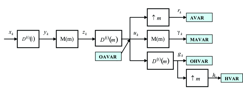
Figure 1: The processing chain of the stability variances, $M(m)$ is a moving average filter of length $m$. $D^{(n)}(m)$ is a difference filter of order $n$ and lag $m$. $\uparrow m$ is the decimation by a factor $m$ operator.

III-B The Overlapping Allan Variance (OAVAR)

This is a special case of the above processing when the order of the difference filter $n$ is equal to one. The normalization factor ${c_{{1}}}$ is given by equation (21) and is equal to ${\sqrt{2}}$. The filter ${d_{k}^{{(2)}}}$ of equation (46) is equal to ${{\delta}_{k}-2{\delta}_{{k+m}}+{\delta}_{{k+2m}}}$. The signal ${u_{k}}$ is given by:

$$u_{k}=\frac{1}{m\sqrt{2}}\left(x_{{k+2m}}-2x_{{k+m}}+x_{k}\right).$$ (62)

Let $N$ the length of the discrete time series ${y_{k}}$. The ${d_{k}^{{(2)}}}$ filter length is $2m$ and the output ${u_{k}}$ length is $N-2m+1$.

According to equation (48), the sample variance of ${u_{k}}$ is:

$$\textrm{OAVAR}(m)={\hat{{\sigma}}}_{{u}}^{2}\left(m\right)$$ (63)

$$=\frac{1}{2m^{2}\left(N-2m+1\right)}\sum_{k=0}^{N-2m}\left(x_{{k+2m}}-2x_{{k+m}}+x_{k}\right)^{2}$$

which is the classical estimator of the Overlapping estimator of Allan Variance [20].

The computation in (63) from ${x_{k}}$ requires four additions and one multiplication for each term inside the sum. The sum over $k$ requires $N-2m+1$ addition. The whole computation requires roughly $5\times N$ operation and is linear in $N$.

When the available measurement are frequency fluctuations ( $\left|y_{k}\right|$), it’s more efficient (in number of floating point operations but not in memory use) to compute the phase signal ${x_{k}}$ using (34) and then use (63) to compute the OAVAR variance than to compute ${z_{k}}$ from ${y_{k}}$ and then ${u_{k}}$.

Replacing $n$ by 1 in equation (54) we get an expression of the Overlapped Allan Variance versus the one-sided set of DFT coefficient ${{\tilde{Y}}_{k}}$ of the measurement time series ${y_{k}}$ by:

$$\textrm{OAVAR}(m)_{F}={\hat{{\sigma}}}_{{F,u}}^{2}\left(m\right)=\frac{4}{m^{2}N^{2}}\sum_{k=0}^{P}\frac{\sin^{{4}}\left(\frac{\pi{km}}{N}\right)}{\sin^{2}\left(\frac{{{\pi}k}}{N}\right)}|{\tilde{Y}}_{k}|^{2}.$$ (64)

The DFT computation complexity is N log(N) when using a Fast Fourier Transform (FFT) algorithm. But the most CPU consuming in (64) is the computation of the sine trigonometric functions inside the sum symbol. It’s trivial that the computation using equation (63) is more efficient than using equation (64).

It’s worth recalling that the discrete time formula (63) use $N-2m+1$ terms. The largest acceptable $m$ value is $N/2$. In this case the variance is estimated from one sample only. The DFT formula (64) use $P$ terms whatever the $m$ value. When $m=N/2$ the half of the sine terms in (64) is null. The computation of the confidence levels when using equation (64) has shown that the confidence levels are better than that of the discrete time formula of equation (63) because filtering in frequency domain use all the available samples while filtering in the time domain use $N$ minus the filter length samples. In fact, Filtering in the DFT domain is done by multiplication of the DFT. This multiplication is equivalent to circular convolution in the time domain. Circular or cyclic convolution of two signal of length $N$ is equivalent to classical sum convolution with indices modulo $N$. This means that DFT formula (64) is equivalent to a kind of Total Variance [1] where the series ${y_{k}}$ is extended by periodic (circular) repetitions. The Total Hadamard Variance [9] uses an extended version of ${y_{k}}$ where the extension use a reflected copy of ${y_{k}}$.

III-C The “Non Overlapping” Allan Variance (AVAR)

The “Non overlapping” Allan variance is a special case of the classical Allan Variance that doesn’t use overlapped values when computing ${\sum{u_{k}^{2}}}$ in the sample variance of ${u_{k}}$. This means that only $(N-2m+1)/m$ values are considered when forming the sum.

In other words, the Allan Variance AVAR is obtained from ${u_{k}}$ by a decimation operation of order $m$ (See Figure 1). If we start the decimation at $k=0$ we can use $N/m-1$ values. The decimated signal ${r_{k}}$ is given by:

$${r_{k}=u_{{km}}\;,\;0\leq k\leq\frac{N}{m}-2}.$$ (65)

Replacing (65) in (63) we get the non overlapping Allan variance as the sample variance of ${r_{k}}$:

$$\textrm{AVAR}(m)=\hat{\sigma}_{r}^{2}(m)$$ (66)

$$=\frac{1}{2m(N-m)}\sum_{k=0}^{N/m-2}\left(x_{(k+2)m}-2x_{(k+1)m}+x_{km}\right)^{2}$$

It’s obvious that the AVAR requires less computation than the OAVAR. In fact, for each $m$ value there are $N/m-1$ terms. The largest acceptable $m$ value is $N/2$. In this case the sample variance is estimated from one sample only. The confidence levels for AVAR and OAVAR are equals for $m=1$ and $m=N/2$. Values of m between $m=1$ and $m=N/2$ give a better confidence levels in the OAVAR than in the AVAR variance.

Because the OAVAR confidence levels are globally better than those of AVAR , the only interest to use the AVAR instead of OAVAR is its computation efficiency.

Though decimation operation of equation (65) is very simple in the time domain it has no interest in the frequency domain. In fact, the computation of the DFT coefficient ${R_{k}}$ of ${r_{k}}$ versus the DFT coefficients of ${u_{k}}$ is given by:

$$R_{n}=\frac{1}{m}\sum_{k=0}^{m-1}U_{\left(n-pN/m\right)}\quad\textrm{Modulo }\quad N.$$ (67)

Computing the sample variance of ${r_{k}}$ according to (52) require an additional loop to compute ${R_{k}}$. For this reason we don’t propose a formula to compute the AVAR in the frequency domain as we did for OAVAR in equation (64).

III-D The Modified Allan Variance (MAVAR)

The modified Allan Variance was introduced [5] to overcome the relatively poor discrimination capability of the Allan variance against white and flicker phase noise.

Let ${{\gamma}_{k}}$ be the signal obtained from ${u_{k}}$ by a moving average filter $M(m)$ of length $m$ (See Figure 1):

$${\gamma}_{k}=\frac{1}{m}\left(u_{k}+u_{{k+1}}+\cdots+u_{{k+m-1}}\right).$$ (68)

Using ${u_{k}}$ expression from (62) in (68) we get:

$$\sqrt{2}m^{2}\gamma_{k} = x_{k}+\cdots+x_{{k+m-1}}$$ (69)

$$-2\left(x_{{k+m}}+\cdots+x_{{k+2m-1}}\right)$$

$$+x_{{k+2m}}+\cdots+x_{{k+3m-1}}.$$

Using this expression directly to compute ${{\gamma}_{k}}$ requires a summation loop with $3*(m+1)$ floating point operation. The biggest acceptable $m$ value in this equation is $m=N/3$. This yields a computation complexity of ${N^{2}}$.

In order to reduce the computation complexity we propose a recursive formula. Expressing ${A_{{k+1}}=\sqrt{2}m^{2}{\gamma}_{{k+1}}}$ using equation (69) we can write:

$$A_{{k+1}}=A_{k}+x_{{k+3m}}-3x_{{k+2m}}+3x_{{k+m}}-x_{k}$$ (70)

with a starting $A_{0}$ value computed using (69) with $k=0$.

Allan [21] already proposed a recursive method in order to reduce the computation complexity of the Modified Allan Variance without giving the details of the recursive equation.

The computation complexity of ${A_{k}}$ according to (70) is linear in $N$.

The length of the time series ${u_{k}}$ is $N-2m+1$ and the length of the filter $M(m)$ is $m$. we conclude that the length of ${{\gamma}_{k}}$ is $N-3m+2$.

The Modified Allan Variance MAVAR is the sample variance of ${{\gamma}_{k}}$:

$$\textrm{MAVAR}(m)={\hat{{\sigma}}}_{{\gamma}}^{2}\left(m\right)=\frac{1}{2m^{{4}}\left(N-3m+2\right)}\sum_{k=0}^{N-3m-1}|A_{k}|^{2}.$$ (71)

The PSD ${S_{{\gamma}}\left(f\right)}$ of the discrete time signal ${{\gamma}_{k}}$ is related to that of ${y_{k}}$ by:

$$S_{{\gamma}}\left(f\right) = |M^{*}\left(f\right)D^{{*}}\left(f\right)M^{*}\left(f\right)|^{2}S_{y}\left(f\right)$$ (72)

$$= \frac{2\sin^{{6}}\left(\pi{mf}\right)}{m^{{4}}\sin^{{4}}\left({{\pi}f}\right)}S_{y}\left(f\right).$$

The DFT coefficients ${{\Gamma}_{{n}}}$ of the series ${{\gamma}_{k}}$ are given by:

$${\Gamma}_{{n}}=M^{*}\left(\frac{n}{N}\right)D^{{*}}\left(\frac{n}{N}\right)M^{*}\left(\frac{n}{N}\right)Y_{{n}}=\frac{\sqrt{2}\sin^{{3}}\left({{\pi}m}\frac{n}{N}\right)}{m^{2}\sin^{2}\left(\pi\frac{n}{N}\right)}Y_{{n}}.$$ (73)

According to the Parseval’s equation (52) for the series ${{\gamma}_{k}}$ we can express the MAVAR versus the one-sided set of DFT coefficients of the measured signal by:

$$\textrm{MAVAR}(m)_{F}={\hat{{\sigma}}}_{{F,\gamma}}^{2}\left(m\right)=\frac{4}{m^{{4}}N^{2}}\sum_{k=0}^{P}\frac{\sin^{{6}}\left(\frac{\pi{mk}}{N}\right)}{\sin^{{4}}\left(\frac{{{\pi}k}}{N}\right)}|{\tilde{Y}}_{k}|^{2}.$$ (74)

As for the OAVAR formula in the frequency domain this equation is an estimator of the MAVAR in the frequency domain. The main difference with the discrete time formula (71) is the number of terms involved in the sum: $P$ in the case of equation (74) and $N-2m+1$ in equation (71).

III-E The Overlapping Hadamard Variance (OHVAR)

This is a special case of the above processing when the order of the difference filter $n$ is equal to two. The normalization factor ${c_{{2}}}$ is given by equation (21) and is equal to ${\sqrt{6}}$. The filter ${d_{k}^{{(3)}}}$ of equation (46) is equal to ${{\delta}_{k}-3{\delta}_{{k+m}}+3{\delta}_{{k+2m}}-{\delta}_{{k+4m}}}$. We denote ${g_{k}=u_{k}}$ where ${u_{k}}$ is given by (46) with $n=2$:

$${g_{k}=\frac{1}{\sqrt{6}m}\left(x_{{k+3m}}-3x_{{k+2m}}+3x_{{k+m}}-x_{k}\right)}.$$ (75)

Let $N$ the length of the discrete time series ${y_{k}}$. The ${d_{k}^{{(3)}}}$ filter length is 3m and the output ${g_{k}}$ length is $N-3m+1$.

The Overlapping Hadamard Variance is the sample variance of ${g_{k}}$:

$$\textrm{OHVAR}(m) = {\hat{{\sigma}}}_{{g}}^{2}\left(m\right)$$

$$= \frac{1}{6m^{2}\left(N-3m+1\right)}$$

$$\times\sum_{k=0}^{N-3m}{\left(x_{{k+3m}}-3x_{{k+2m}}+3x_{{k+m}}-x_{k}\right)^{2}}.$$

Replacing $n$ by 2 in equation (54) we get an expression of the Overlapping Hadamard Variance versus the one-sided set of DFT coefficient $\tilde{Y}_{k}$ of the measurement time series ${y_{k}}$ by:

$$\textrm{OHVAR}_{F}\left(m\right)={\hat{{\sigma}}}_{{F,g}}^{2}\left(m\right)=\frac{16}{3m^{2}N^{2}}\sum_{k=0}^{P}{\frac{\sin^{{6}}\left(\frac{\pi{mk}}{N}\right)}{\sin^{2}\left(\frac{{{\pi}k}}{N}\right)}|{\tilde{Y}}_{k}|^{2}}.$$ (77)

As for formulas (64) and (74), equation (77) is a new formula that allows to compute the OHAVAR in the frequency domain.

It’s clear from equation (75) that the Hadamard variance estimator in the time domain cancels linear drifts. In fact, if ${y_{k}=k}$ then ${x_{k}=k\left(k-1\right)/2}$ according to equation (34). Replacing this value in equation (75) leads to ${g_{k}=0}$ whatever the value of m.

III-F The Hadamard Variance (HVAR)

The Hadamard variance is a special case of the Overlapping Hadamard Variance that doesn’t use overlapped values when computing ${\sum{g_{k}^{2}}}$ in the sample variance of ${g_{k}}$. This means that only $(N-3m+1)/m$ values are considered when forming the sum.

In other words, the Hadamard Variance HVAR is obtained from ${g_{k}}$ by a decimation operation of order $m$ (See Figure 1). If we start the decimation at $k=0$ we can use $N/m-2$ values. The decimated signal ${h_{k}}$ is given by:

$${h_{k}=g_{{km}}\;,\;0\leq k\leq\frac{N}{m}-3}.$$ (78)

Replacing (78) in (75) we get the non overlapping Hadamard variance as the sample variance of ${h_{k}}$:

$$\textrm{HVAR}(m) = {\hat{{\sigma}}}_{{h}}^{2}\left(m\right)$$ (79)

$$= \frac{1}{6m\left(N-2m\right)}\sum_{k=0}^{N/m-3}\left(x_{{(k+3)m}}\right.$$

$$\left.-3x_{{(k+2)m}}+3x_{{(k+1)m}}-x_{{km}}\right)^{2}.$$

As for the Non Overlapping Allan Variance AVAR we don’t propose a formula in the frequency domain for HVAR because the decimation operation doesn’t simplify computation in the frequency domain as it does in the time-domain.

IV Frequency variances Equivalent Degree of Freedom

We can express the frequency-domain variance estimator by the general form :

$$\Psi=\sum_{k=0}^{P}{H_{k}(n,m)\frac{{\left|\tilde{Y}\right|^{2}}}{N}}$$ (80)

Where $n$ is the difference filter order, $m$ is the averaging factor and $H_{k}(n,m)$ is given by :

$$H_{k}(n,m)=\frac{2^{2n+1}}{c_{n}^{2}m^{2}N}\frac{\sin^{2n+2}\left(\frac{\pi km}{N}\right)}{\sin^{2}\left(\frac{\pi k}{N}\right)}$$ (81)

for the non-modified variances and :

$$H_{k}(n,m)=\frac{2^{2n+1}}{c_{n}^{2}m^{4}N}\frac{\sin^{2n+4}\left(\frac{\pi km}{N}\right)}{\sin^{4}\left(\frac{\pi k}{N}\right)}$$ (82)

for the modified variances.

The quantity $\left|\tilde{Y}\right|^{2}/N$ is the periodogram $P(f)$ evaluated at discrete frequency values $f_{k}=$$\frac{k}{N}$. Equation ( 80 ) can be written as :

$$\Psi=\sum_{k=0}^{P}{H_{k}(n,m)P\left(f_{k}\right)}$$ (83)

The periodogram $P(f)$  is an estimator of the PSD $S_{y}(f)$ : $P(f)=\hat{S}\left(f\right)$ .

We estimate the Equivalent Degree of Freedom (edf) of $\Psi$ by :

$$edf=\frac{2\left(E\left(\Psi\right)\right)^{2}}{Var\left(\Psi\right)}$$ (84)

The mean value $E\left(\Psi\right)$ is given by :

$$E\left(\Psi\right)=\sum_{k=0}^{P}{H_{k}(n,m)E\left(P\left(f_{k}\right)\right)}$$ (85)

It is well know that the periodogram is a biased estimator of the PSD $S_{y}(f)$ and that :

$$E\left(P\left(f\right)\right)=W_{B}\left(f\right)\otimes S\left(f\right)$$ (86)

Where $W_{B}\left(f\right)$ is the Bartlett window defined by :

$$W_{B}\left(f\right)=\frac{\sin^{2}\left(\pi Nf\right)}{N\sin^{2}\left(\pi f\right)}$$ (87)

and $\otimes$ denotes the circular convolution defined by :

$$W_{B}\left(f\right)\otimes S\left(f\right)=\int_{-1/2}^{1/2}W_{B}\left(\theta\right)S\left(f-\theta\right)d\theta$$ (88)

It’s clear that the periodogram is asymptotically unbiased since as $N$ becomes very large $W_{B}\left(f\right)$ approaches an impulse in the frequency domain. Then we can write for large N :

$$E\left(\Psi\right)\cong\sum_{k=0}^{P}{H_{k}(n,m)S\left(f_{k}\right)}$$ (89)

and for power law spectrum :

$$E\left(\Psi\right)=h_{\alpha}\sum_{k=0}^{P}{H_{k}(n,m)\left(\frac{k}{2N}\right)^{\alpha}}$$ (90)

The variance $Var\left(\Psi\right)$ is given by :

$$\begin{array}[]{c}Var\left(\Psi\right)=E\left(\Psi^{2}\right)\\ =\sum\limits_{k=0}^{P}\sum\limits_{j=0}^{P}{H_{k}(n,m)H_{j}(n,m)Cov\left(P\left(f_{k}\right),P\left(f_{j}\right)\right)}\end{array}$$ (91)

The covariance of the periodogram is given by :

$$Cov\left(P\left(f_{1}\right),P\left(f_{2}\right)\right)=$$ (92)

$$S_{y}\left(f_{1}\right)S_{y}\left(f_{2}\right)\left(\frac{\sin\left(\pi N\left(f_{1}-f_{2}\right)\right)}{N\sin\left(\pi\left(f_{1}-f_{2}\right)\right)}\right)^{2}$$

Replacing $f_{1}$ by $f_{k}=\frac{k}{N}$ and $f_{2}$ by $f_{j}=\frac{j}{N}$ in equation we get :

$$Cov\left(P\left(f_{k}\right),P\left(f_{j}\right)\right)=$$ (93)

$$S_{y}\left(f_{k}\right)S_{y}\left(f_{j}\right)\left(\frac{\sin^{2}\left(\pi\left(k-j\right)\right)}{N^{2}\sin^{2}\left(\frac{\pi}{N}\left(k-j\right)\right)}\right)$$

Therefore, the covariance (93) is is seen to go to zero when $k\neq j$ . The variance is therefore :

$$Var(\Psi)=\sum_{k=0}^{P}H_{k}^{2}(n,m)S_{y}^{2}(f_{k})$$ (94)

The edf is, according to (84), given by :

$$edf=\frac{2(\sum_{k=0}^{P}H_{k}(n,m)S_{y}(f_{k}))^{2}}{\sum_{k=0}^{P}H_{k}^{2}(n,m)S_{y}^{2}(f_{k})}$$ (95)

For power law spectrum we get :

$$edf=\frac{2(\sum_{k=0}^{P}k^{\alpha}H_{k}(n,m))^{2}}{\sum_{k=0}^{P}k^{2\alpha}H_{k}^{2}(n,m)}$$ (96)

With $H_{k}\left(n,m\right)$ given by (82) for the modified variances and (81) for the non-modified variances.

V Time Domain versus Frequency Domain: Numerical Results

We have simulated time series data ${y_{k}}$ of length $N=400000$, $2000000$ and $65536$ for the different power law spectra for ${-4\leq\alpha\leq 2}$. Table III and IV show the computation time on a personnal computer (pentium IV or equivalent @ 2.8 GHz) in ms of the different stability variances mentioned in this paper. The computation time of the FFT was included in the computation time of the frequency variances.

Table III: Computation time in ms of the different stability variances, $N=400000$

	AVAR	OAVAR	MAVAR	HVAR	OHVAR
Time Domain	16	47	78	16	47
Frequency Domain	–	265	265	–	265

Table IV: Computation time in ms of the different stability variances, $N=2000000$

	AVAR	OAVAR	MAVAR	HVAR	OHVAR
Time Domain	63	265	484	63	360
Frequency Domain	–	1453	1500	–	1485

For the computation in the frequency domain we used the FFT algorithm of Cooley and Tuckey[22]. The FFT computation time is 45 ms for $N=400000$ and 250 ms for $N=2000000$.

We presented in equation (54) a new way to compute the different stability variances using the DFT of the data. We demonstrated that this equation is equivalent to the equations in the time domain with a slight difference in the number of samples when computing the sample variance. For example, equation (63) in the time domain uses only unambiguous samples in the sense that a filter of length $2m$ will produce $N-2m+1$ unambiguous output samples when applied to an input data of length $N$.

In the following we present numerical results of the different frequency domain variances estimators presented in this paper. The error bars on the plots were computed using one sigma Chi-squared $\chi^{2}$distribution with an equivalent degree of freedom (edf) estimated by making Monte Carlo simulations of 1000 trials.

V-A OAVAR

Figure (2) depicts the edf of the Overlapping Allan Variance computed in the frequency domain (F-OAVAR) for three noise types: a White frequency noise (WHFM), a Flicker frequency noise (FLFM) and a Random Walk frequency noise (RWFM). It shows a very good agreement between the theoretical edf formula of equation (96) and the edf obtained by Monte Carlo simulations.

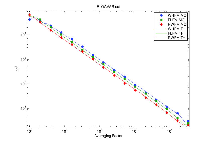
Figure 2: F-OAVAR edf for three noise types for sequences of length $N=65536$. WHFM for White frequency noise, FLFM for Flicker frequency noise and RWFM for Random Walk frequency noise. The continous lines (denoted “TH” on the Figure legend) represent the theoretical edf computed by equation (96). The symbols (denoted “MC” on the Figure legend) represent the edf obtained by Monte Carlo simulation with 1000 trials.

Figure 3: OAVAR computed in the time domain and in the frequency domain for a White Frequency Noise sequence of length $N=65536$. The spectral OAVAR estimates were slightly shifted in order to be distinguished from the time OAVAR estimates. The dashed continuous line represents the theoretical response $h_{0}/(2\tau)$.

Figure (3) compares the Overlapping Allan variance of a white frequency noise sequence computed in the time domain and in the frequency domain from relationship (64). No bias is visible between these computations and the theoretical response (less than 1 %). On the other side, the error bars of OAVAR computed in the frequency domain are clearly smaller as the ones of OAVAR computed in the time domain, as expected in section III-B. Table V shows the equivalent degrees of freedom (edf) of the Total Variance and the OAVAR estimates in the time domain (T-OAVAR) and in the frequency domain (F-OAVAR), assuming a Chi-square statistics [23]. For the highest $\tau$ value ($\tau=N/2$), the edf of the spectral estimate is 3 times higher than the edf of the time estimate, i.e. the spectral estimate is $\sqrt{3}$ times more accurate than the time estimate.

Table V: Comparison of the equivalent degrees of freedom (edf) of the time T-OAVAR estimates, the spectral F-OAVAR estimates and the Total variance estimates for a White Frequency Noise sequence of length $N=65536$.

$\mathbf{\tau}$	T-OAVAR	F-OAVAR	TotVar
1	46591	42297	45368
2	40640	37232	34379
4	24186	23639	22460
8	11870	12338	11451
16	5865	6786	6375
32	2937	3255	2945
64	1493	1515	1555
128	746	740	832
256	383	372	414
512	199	194	215
1024	93	89	104
2048	43	43	53
4096	20	22	26
8192	10	12	12
16384	4	6.4	6.2
32768	1.0	3.0	2.9

Such an advantage is particularly useful for detecting and measuring the level of the low frequency noises (e.g. random walk FM) sooner as with time variances, i.e. for shorter duration. Considering that the edf decreases approximately as $\tau^{-1}$, an estimator with an edf 3 times higher than another one provides a noise level estimation $\sqrt{3}$ times sooner than the other one (e.g. 7 month instead of 1 year) with the same accuracy.

Figure (4) presents a comparaison between the Overlapping Allan variance computed in the frequency domain (F-OAVAR) and the Total variance for three noise types : WHFM, FLFM and RWFM. The upper plot depicts the edf ratio computed using Monte Carlo simulations with 1000 trials. we notice that the edf of the F-OAVAR and the Total variance are nearly identical. The lower plot depicts the bias defined by $Bias=100\times(1-\sqrt{\textrm{F-OAVAR}/\textrm{Totvar}})$. The bias of the F-OAVAR with respect to the Total variance is less than 10%.

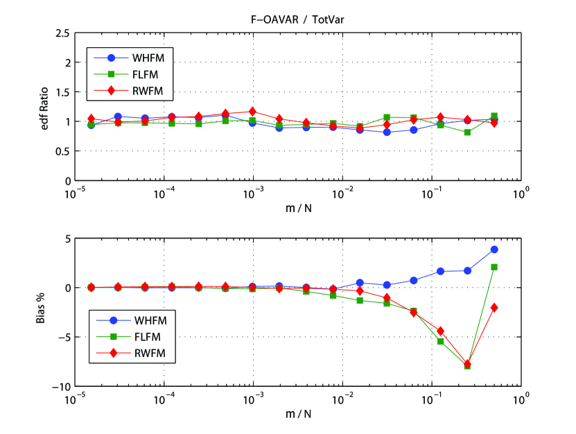
Figure 4: Comparaison of the F-OAVAR and the Total variance for three noise types. The upper plot depicts the edf ratio and the lower plot depicts the bias. $N=56536$. Results were obtained using Monte Carlo with 1000 trials.

In the same way, figure (5) presents a comparaison between the Overlapping Allan variance computed in the frequency domain and the classical Overlapping Allan variance computed in the time domain. The upper plot shows that the F-OAVAR edf is two to three times higher than the edf of the T-OAVAR for the higher $\tau$ value ($\tau=N/2$) .The lower plot depicts the bias defined by $Bias=100\times(1-\sqrt{\mathrm{\textrm{F-OAVAR}}/\mathrm{\textrm{T-OAVAR}}})$.

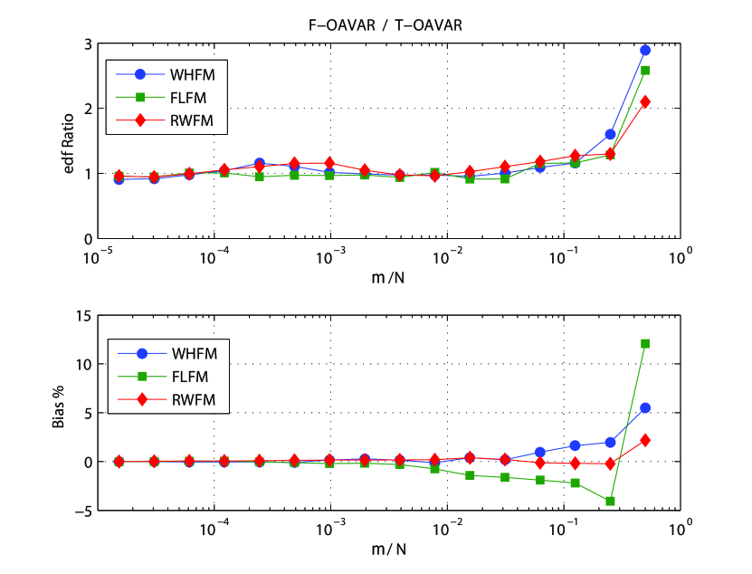
Figure 5: Comparaison of the F-OAVAR and the T-OAVAR for three noise types. The upper plot depicts the edf ratio and the lower plot depicts the bias. $N=56536$. Results were obtained using Monte Carlo with 1000 trials.

Figure (6) shows the Total Variance, the Overalpping Allan Variance computed in the time domain (T-OAVAR) and in the frequency domain (F-OAVAR) for a White frequence noise and a flicker noise with a linear frequency drift. The added linear drifts is equal to $D(t)=15t$ . Like the the Total variance and the classical Allan variance, the F-OAVAR does not cancel the linear drift. We can notice also that the F-OAVAR for a linear drift varies as $\tau$ , while the Total variance and the T-OAVAR vary as $\tau^{2}$.

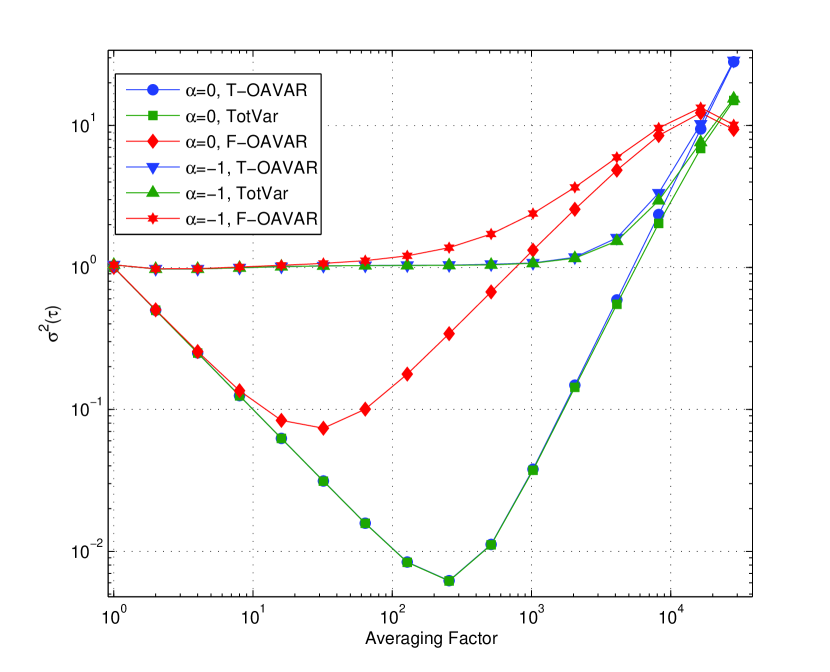
Figure 6: The T-OAVAR, the Total variance and the F-OAVAR for a White frequence noise ($\alpha=0$) and a Ficker frequency noise ($\alpha=-1$) . A linear frequency drift was added to the noise sequences of length $N=56536$ (Monte Carlo trials = 1000).

Unfortunately, the last result shows that the computation of OAVAR in the frequency domain presents a severe drawback: it is unable to discriminate between a linear frequency drift and a $f^{-2}$ frequency noise (random walk FM). This effect is due to the assumption of periodicity of the sequence implicitely induced by the use of the FFT algorithm. Figure 7-A shows that connecting the last sample to the first one may induce a high edge, altering the variance measurements. So we decided to process the frequency deviation sequence with 2 different ways:

• by removing the linear drift of this sequence (see figure 7-B; let us notice that there is still an edge at the end of the sequence). The removed line is estimated by a least squares fit of the data sequence to a line.

• by circularizing the sequence (see figure 7-C), i.e. by removing the linear drift in such a way that the last sample of the residuals is equal to the first one. Denoting by $D(t)=a\cdot t+b$ the drift we have to substract from the sequence, the linear coefficient $a$ is then:

  $$a=\frac{y_{N}-y_{1}}{t_{N}-t_{1}}$$ (97)

  and the constant term $b$ may be choosen equal to 0 since OAVAR is not sensitive to additive constants.

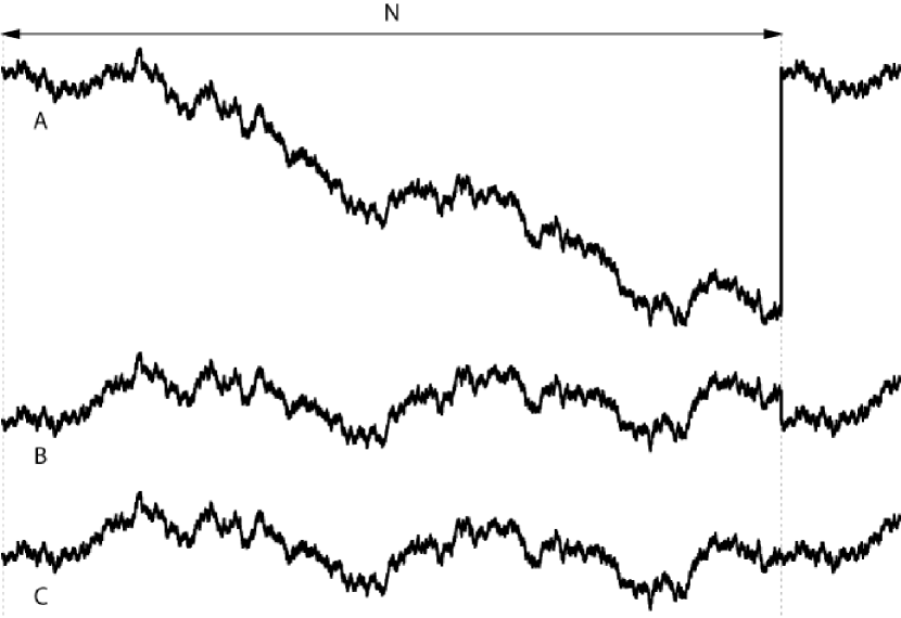
Figure 7: Random Walk Frequency Noise sequence: rough (A), drift removed (B) and circularized (C).

It is worth recalling that Figure (7) shows the side effect of periodization (induced by multiplication in the discret frequency domain) of a sequence without processing, after a line removal, and after circularization. But when computing the frequency domain variances we don’t realize any extension of data manually as done in the computation of the Total variance.

Table (VI) compares the edf of the OAVAR for a Random Walk Frequency Noise computed after these processings. The best estimates are obtained by using the circularized sequence since the edf of the estimates are higher than for for the sequence after removing a linear frequency drift. Thus, the edf of the last estimate ($\tau=N/2$) is 2 times higher than the one of the estimate obtained in the time domain. This means that this estimate provides a noise level estimation $\sqrt{2}$ times sooner than the estimate computed in the time domain (e.g. 265 days instead of 1 year) with the same accuracy.

Table VI: Comparison of the equivalent degrees of freedom of the time OAVAR estimates and the spectral OAVAR estimates rough, after removing a linear drift and after circularizing the sequence for a Random Walk Frequency Noise sequence of length $N=65536$.

$\mathbf{\tau}$	Time OAVAR	Spectral OAVAR
		rough	without drift	circularized
1	68540	65660	39	56735
2	35289	33269	39	27589
4	15498	15410	39	13009
8	7324	7725	38	6392
16	3621	3997	38	3258
32	1812	2091	37	1737
64	900	1040	36	860
128	455	477	35	436
256	225	219	34	224
512	110	106	31	109
1024	52	54	25	50
2048	25	28	17	23
4096	12	14	10	11
8192	5.3	6.7	4.8	5.3
16384	2.4	3.1	2.0	2.6
32768	1.0	2.0	1.5	2.1

However, applying the circularization processing to another type of noise induced is a bias that has the same characteristic as a linear frequency drift on an Allan variance plot. Beside the $\tau^{-1}$ behaviour characteristic of a white FM, figure 8 exhibits the $\tau$ signature of a linear frequency drift in the Allan variance curve of the circularized sequence. Let us also notice the very long errorbars of the circularized sequence estimates. Therefore, the circularization process cannot be used in a real frequency deviation sequence which contains always different types of noise. Thus, we recommand to apply the spectral OAVAR over the residuals of a frequency deviation sequence, after removing the linear frequency drift. For a random walk FM, the estimate of OAVAR computed in the frequency domain after drift removal has an edf 1.5 times higher than the classical time domain OAVAR. It means that spectral OAVAR after drift removal is able to measure the random walk level of a sequence $\sqrt{1.5}$ times sooner than time OAVAR (e.g. 300 days instead of 1 year).

Figure 8: OAVAR for a White Frequency Noise sequence of length $N=65536$ computed in the time domain and in the frequency domain, rough, after removing the linear frequency drift and after circularizing the sequence.

Figure (9) compares the F-OAVAR variance computed after linear drift removal by least squares fit and the classical T-OAVAR variance. As shown in Table (VI) the upper plot shows that the edf of the F-OAVAR after drift removal for a Random Walk noise is less than the edf of the T-OAVAR for small $\tau$ values. The lower plot shows that the F-OAVAR presents a bias of -10% for Random Walk noise. This bias can be explained by the fact the drift removal from a Random Walk sequance alters the spectrum of the noise at all the frequency values because a Random Walk contains a kind of linear drift feature intrinsicly.

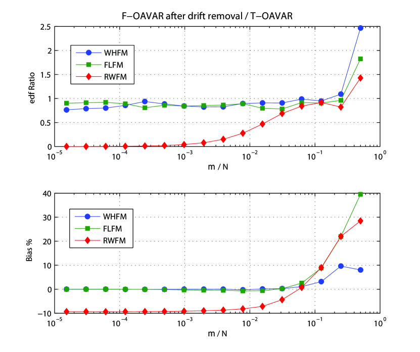
Figure 9: Comparaison of the F-OAVAR computed after drift removal from noise sequences by least squares fit and the classical T-OAVAR for three noise types. The upper plot depicts the edf ratio and the lower plot depicts the bias. $N=56536$. Results were obtained using Monte Carlo with 1000 trials.

Let us remember that for a sequence without random walk FM (for atomic clocks), OAVAR computed in the frequency domain may be used directly and is more accurate than OAVAR computed in the time domain.

V-B OHVAR

Figure (10) depicts the edf of the Overlapping Hadamard variance computed in the frequency domain F-OHVAR. It shows a very good agreement between the theoretical edf formula of equation (96) and the edf obtained by Monte Carlo simulations.

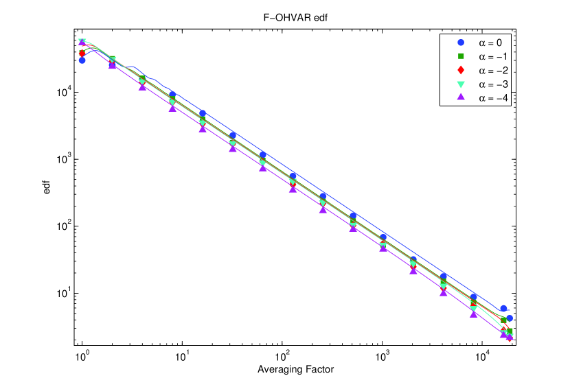
Figure 10: F-OHVAR edf for five noise types ($\alpha$ from -4 to 0) for sequences of length $N=65536$. The continous lines represent the theoretical edf computed by equation (96). The symbols represent the edf obtained by Monte Carlo simulation with 1000 trials.

Figure (11) shows that edf of the OHVAR estimator in the frequency domain is 2 to 4.5 higher than the edf of the classical OHVAR for the higher $\tau=N/3$ value. The lower plot depicts the bias defined by $Bias=100\times(1-\sqrt{\mathrm{\textrm{F-OHVAR}}/\mathrm{\textrm{T-OHVAR}}})$. It is less than 10% for the five noise types and for all the $\tau$ values.

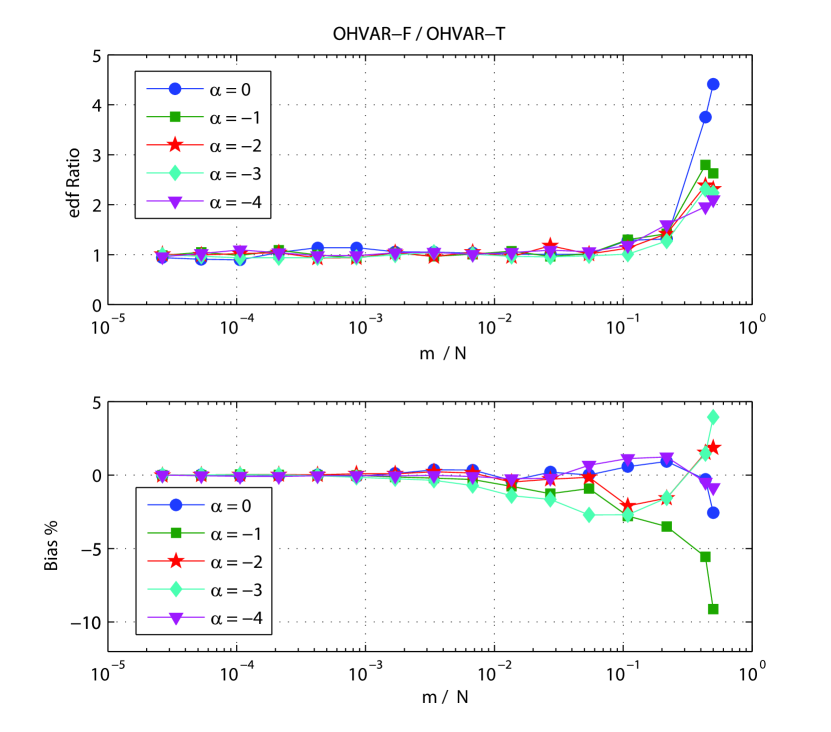
Figure 11: Comparaison of the F-OHVAR and the T-OHVAR for five noise types. The upper plot depicts the edf ratio and the lower plot depicts the bias. $N=56536$. Results were obtained using Monte Carlo with 1000 trials.

The Hadamard variance is not sensitive to linear frequency drifts. However, computing OHVAR in the frequency domain by using a FFT assumes also the periodicity of the sequence and may induce a high edge by connecting the last sample to the first one (see figure 7-A). We performed then the same processings as previously in order to compare the effects of the drift removal and of the circularization of the sequence. For OHVAR also, the circularization should not be recommanded for processing frequency deviation sequences because it is only useful for noises with $\alpha\leq-2$ and it degrades the variance estimates for the noises with $\alpha>-2$ . On the other hand, the drift removal by substracting the best least squares line from the data gives good results for noises with $\alpha>-2$ . Hence, it is better to use the F-OHVAR directly without preprocessing in order to get better statistics than the T-OHVAR if the data does not contain a linear drift.

V-C MAVAR

Figure (12) shows a comparaison of the modified Allan variance computed in the frequency domain (F-MAVAR) and in the time domain (T-MAVAR) for five noise types with $\alpha$ from -2 to +2. We can notice clearly a huge bias of the F-MAVAR for $\alpha=+2$ .

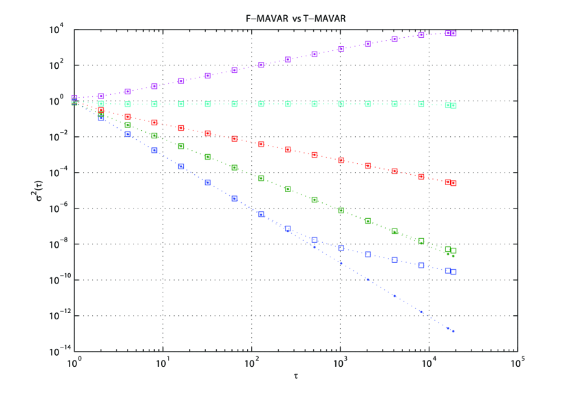
Figure 12: F-MAVAR and T-MAVAR for five noise types ($\alpha$ from -2 to +2) for sequences of length $N=65536$. The squares represent the F-MAVAR values and the dots represent the T-MAVAR values. Monte Carlo simulation with 1000 trials.

For this reason, the use of MAVAR computed in the frequency domain should be avoided.

VI Conclusion

We have presented a filter approach to analyze the different known frequency stability variances. Using this approach we derived formulae in the time domain identical to those known in the literature. We also demonstrated for the first time that the computation of these variances can be done in the frequency domain using a Discrete Fourier Transform of the studied signals. Such a computation provides estimates with better accuracy than the ones computed in the time domain, allowing the measurement of the low frequency noise levels sooner, i.e. with a shorter sequence. This advantage is particularly useful for studying the long term stability of atomic clocks. However, in the presence of linear drift, the periodicity of the sequence implicitely assumed by the use of the FFT algorithm may induce edges which degrade variance measurements if a random walk FM is present in the sequence. We have demonstrated that, in this case, we must first remove the linear frequency drift on a sequence before to compute a variance in the frequency domain. Our work has proved that OAVAR computed in the frequency domain is the estimator which gives the quickest low frequency noise level (9 month instead of 1 year). New estimators improving these characteristics with a more simple transfer function will be described in another paper [24].

Appendix : Equivalence of the Discrete-Time and the Continuous-Time variances

We have assumed $T=1$ in (44). Without this assumption the variance ${{\sigma}_{{u}}^{2}\left(m\right)}$could be written using (31):

$${\sigma}_{{u}}^{2}\left(m\right) = T\int_{-\frac{1}{2T}}^{+\frac{1}{2T}}S_{{u}}^{TS}(f)df$$

$$= T\frac{2^{2n}}{c_{n}^{2}m^{2}}\int_{-\frac{1}{2T}}^{+\frac{1}{2T}}\frac{\sin^{2n+2}\left(\pi fmT\right)}{\sin^{2}\left(\pi{fT}\right)}S_{y}^{TS}\left(f\right)df.$$

Using expression (29) of ${S_{y}(f)}$ in (Appendix : Equivalence of the Discrete-Time and the Continuous-Time variances) we can write:

$$\sigma_{u}^{2}(m) = \frac{2^{2n}}{c_{n}^{2}m^{2}}\int_{-\frac{1}{2T}}^{+\frac{1}{2T}}\left\{\frac{\sin^{{2n+2}}\left(\pi{fmT}\right)}{\sin^{2}\left(\pi{fT}\right)}\right.$$

$$\left.\times\sum_{n}S_{Y}^{TS}\left(f-nf_{s}\right)\frac{\sin^{2}\left[\pi T\left(f-nf_{s}\right)\right]}{\left[\pi T\left(f-nf_{s}\right)\right]^{2}}\right\}df.$$

The sine functions outside the sum sign are periodic, they can be passed inside the sum sign. Doing this and making the variable change ${\nu=f-nf_{s}}$ we can write:

$$\sigma_{u}^{2}(m) = \frac{2^{{2n}}}{c_{{n}}^{2}m^{2}}\sum_{k=-\infty}^{+\infty}{\int_{-\frac{1}{2T}-\frac{n}{T}}^{+\frac{1}{2T}-\frac{n}{T}}}\left[\frac{\sin^{{2n+2}}\left(\pi\nu mT\right)}{\sin^{2}\left(\pi\nu T\right)}\right.$$ (100)

$$\left.\times\frac{\sin^{2}\left(\pi T\nu\right)}{\left(\pi T\nu\right)^{2}}S_{Y}^{TS}(\nu)\right]d\nu$$

where we have interchanged the sum sign and the integration symbol.

Equation (100) simplifies to:

$${\sigma}_{{u}}^{2}\left(m\right) = \frac{2^{{2n}}}{c_{{n}}^{2}}\int_{-\infty}^{+\infty}\frac{\sin^{{2n+2}}\left(\pi\nu mT\right)}{\left(\pi mT\nu\right)^{2}}S_{Y}^{TS}(\nu)d\nu$$ (101)

$$= {\sigma}_{{U}}^{2}\left(\tau\right)_{{(n)}}|_{{\tau={mT}}}.$$

The only difference between (101) and (24) is the integration bounds. In equation (24), ${S_{Y}\left(f\right)}$ is the single-sided PSD while ${S_{Y}^{TS}\left(u\right)}$ in (101) is the two-sided PSD. We conclude that (44) and (24) represent the same variance.

References

- [1] C. A. Greenhall, D. A. Howe, and D. B. Percival, “Total variance, an estimator of long-term frequency stability,” IEEE Transactions on Ultrasonics, Ferroelectrics and Frequency Control, vol. UFFC-46, no. 5, pp. 1183–1191, September 1999.
- [2] D. W. Allan, “Statistics of atomic frequency standards,” Proceedings of the IEEE, vol. 54, pp. 221–230, February 1966.
- [3] J. A. Barnes, A. R. Chi, L. S. Cutler, D. J. Healey, D. B. Lesson, T. E. McCunigal, J. A. Mullen, W. L. Smith, R. L. Sydnor, R. Vessot, and G. M. R. Winkler, “Characterization of frequency stability,” IEEE Transactions on Instrumentation and Measurement, vol. IM-20, pp. 105–120, May 1971.
- [4] W. C. Lindsey and C. M. Chie, “Theory of oscillator instability based upon structure function,” Proceedings of the IEEE, vol. 64, pp. 1652–1666, December 1976.
- [5] D. Allan and J. A. Barnes, “A modified “allan variance” with increased oscillator characterization ability,” in Proceedings of the 35 Annual Frequency Control Symposium, Fort Monmouth (NJ, USA), May 1981, pp. 470–475.
- [6] J. Rutman, “Characterization of phase and frequency instabilities in precision frequency sources: fifteen years of progress,” Proceedings of the IEEE, vol. 66, no. 9, pp. 1048–1075, September 1978.
- [7] F. Roddier, Distributions et transformation de Fourier. Paris: McGraw-Hill, 1978.
- [8] A. Papoulis, Probability, Random Variables, and Stochastic Processes, 3 ed. New York: McGraw Hill, 1991.
- [9] D. A. Howe, R. L. Beard, C. A. Greenhall, F. Vernotte, W. J. Riley, and T. K. Peppler, “Enhancements to GPS operations and clock evaluations using a "total" hadamard deviation,” IEEE Transactions on Ultrasonics, Ferroelectrics, and Frequency Control, vol. UFFC-52, no. 8, pp. 1253–1261, August 2005.
- [10] F. Vernotte, “Application of the moment condition to noise simulation and to stability analysis,” IEEE Transactions on Ultrasonics, Ferroelectrics, and Frequency Control, vol. UFFC-49, no. 4, pp. 508–513, April 2002.
- [11] R. Baugh, “Frequency modulation analysis with the hadamard variance,” in Proceedings of the 25 Annual Frequency Control Symposium, June 1971, pp. 222–225.
- [12] E. Boileau and B. Picinbono, “Statistical study of phase fluctuations and oscillator stability,” IEEE Transactions on Instrumentation and Measurement, vol. IM-25, no. 1, pp. 66–75, March 1976.
- [13] T. Walter, “A multi-variance analysis in the time domain,” 24th Annual Precise Time and Time Interval (PTTI) Meeting, pp. 413–424, 1992.
- [14] D. B. Percival and A. T. Walden, Wavelet Methods for Time Series Analysis, ser. Cambridge Series in Statistical and Probabilistic Mathematics. Cambridge: Cambridge University Press, 2000.
- [15] F. Vernotte, G. Zalamansky, and E. Lantz, “Time stability characterization and spectral aliasing. Part I: A time domain approach,” Metrologia, vol. 35, no. 5, pp. 723–730, December 1998.
- [16] ——, “Time stability characterization and spectral aliasing. Part II: A frequency domain approach,” Metrologia, vol. 35, no. 5, pp. 731–738, December 1998.
- [17] D. B. Percival, “Characterization of frequency stability: Frequency-domain estimation of stability measures,” in Proceedings of the IEEE, VOL. 79, NO. 6, July 1991, pp. 961–972.
- [18] P. C. Chang, H. M. Peng, and S. Y. Lin, “Allan variance estimated by phase noise measurements,” 36th Annual Precise Time and Time Interval (PTTI) Meeting, pp. 165–172, 2004.
- [19] F. Vernotte, “Stabilité temporelle des oscillateurs : nouvelles variances, leurs propriétés, leurs applications,” PhD thesis, order N# 199, Université de Franche-Comté, Observatoire de Besançon, February 1991.
- [20] D. A. Howe, D. W. Allan, and J. A. Barnes, “Properties of signal sources and measurement methods,” in Proceedings of the 35 Annual Frequency Control Symposium, Fort Monmouth (NJ, USA), May 1981, pp. A1–A47.
- [21] D. W. Allan, “Time and frequency metrology: current status and future considerations,” 5th EFTF, 1-9, Besançon, 1999.
- [22] J. W. Cooley and J. W. Tukey, “An algorithm for the machine calculation of complex fourier series,” Math. Comput., vol. 19, no. 90, pp. 297–301, April 1965.
- [23] P. Lesage and C. Audoin, “Characterization of frequency stability: uncertainty due to the finite number of measurements,” IEEE Transactions on Instrumentation and Measurement, vol. IM-22, pp. 157–161, June 1973, see also corrections published in 1974, March and 1976, September.
- [24] A. Makdissi, F. Vernotte, and E. Declercq, “Stability variances: New variances in the frequency domain,” To be published.