Shear-Flow Transition: the Basin Boundary

Abstract

The basin of attraction of a stable equilibrium point is investigated for a dynamical system (W97) that has been used to model transition to turbulence in shear flows. The basin boundary contains a linearly unstable equilibrium point $X_{lb}$ which, in the self-sustaining scenario, plays a role in mediating the transition in that transition orbits cluster around its unstable manifold. We find for W97, however, that this role is played not by $X_{lb}$ but rather by a periodic orbit also lying on the basin boundary. Moreover, it appears via numerical computations that all orbits beginning near $X_{lb}$ relaminarize. We offer evidence that this is due to the exquisite narrowness of the complementary region to the basin of attraction in the part of phase space near $X_{lb}$. This further leads to a proposal for understanding the ’edge of chaos’ in terms of more familiar invariant sets of a dynamical system.

MSC numbers:76D05, 76F20

1 Introduction

Experimentally, laminar shear flows undergo transition to turbulence when the relevant parameter, the Reynolds number $R$, exceeds a critical value $R_{c}$. Mathematically, when the Navier-Stokes equations are linearized about the laminar flow, the expected passage from stability to instability at $R_{c}$ is not found. This is the familiar conundrum that linear theory fails to predict the critical value $R_{c}$ (cf., for example, the introductory remarks in [5] for a fuller discussion). A resolution of this conundrum is that the stable, laminar point $O$ possesses a basin of attraction $B$ whose boundary $\partial B$ passes increasingly close to $O$ with increasing $R$, so that perturbations that may be small by laboratory standards are large enough to transgress $\partial B$ for sufficiently large values of $R$.

This idea of describing the problem of shear flows in the language of dynamical-systems theory is an attractive one but has limitations when the model systems are confined to very low dimensions. For example, the debate whether turbulence is transient or not ([4]) can hardly be joined in this context, where $\partial B$ presents a clear boundary between transient and permanent departures from the laminar flow. The present work is nevertheless confined to models of very low dimensions. The motivations are (1) the impression that the nature of the basin of attraction is an important element in the theory, (2) the observation that very little is known about it and (3) the conviction that it would be a good idea to understand the basin and its boundary in low-dimensional systems before proceeding to high-dimensional systems. In this paper we have considered the four-dimension model W97 (as described in [9]) and minor modifications of it.

Some results that may be relevant to higher-dimensional models and to the Navier-Stokes (NS) equations, discussed in more detail in §5, include the structure of the boundary, which implies that the functional form of a perturbation may be as important as its size; that the vicinity of $X_{lb}$ may not be a good place to seek transition; and that the tendency of the complementary region to the basin of attraction to extreme narrowness in some parts of phase space may help to explain the ’edge of chaos’ ([7]) in terms of the more familiar invariant sets of dynamical-systems theory.

The plan of the paper is as follows. We describe the mathematical setting in §2. In §3 we present Waleffe’s model together with diagrams of the boundary of the basin of attraction indicating the periodic orbit that lies on that boundary, and the relaminarization of orbits starting near $X_{lb}$. In §4 we indicate a resolution of this relaminarization in terms of the folded structure of the basin boundary. The concluding section, §5, is devoted to drawing from this resolution a proposed interpretation of the edge of chaos and to brief remarks on the results of this paper and their implications for further study.

2 Mathematical Setting

The Navier-Stokes (NS) equations possess a number of very simple solutions representing laminar shear flows (plane Couette and Poiseuille flow, pipe flow, etc.). When these partial-differential equations are modeled by a finite-dimensional system, the laminar flow can modeled by an equilibrium point of that system, which we’ll take to be the origin of coordinates $O$. Almost all such finite-dimensional systems that have been studied take the form

$$\dot{x}=Ax+b(x),x\in R^{n}$$ (1)

satisfying certain conditions:

1. $A$ is a non-normal, stable matrix.

2. $b(x)$ is quadratic in $x$ and $\sum_{j=1}^{n}x_{j}b_{j}(x)=0.$

This structure can be inferred by a Galerkin projection of the NS equations onto $n$ basis vectors, while taking mild liberties with the boundary conditions.

The stability condition on $A$ implies that its eigenvalues lie in the left half-plane and therefore that the origin $O$ is asymptotically stable. The basin of attraction $B$ of an asymptotically stable equilibrium point is the set with the property that any orbit through a point of $B$ tends to the equilibrium point as $t\to+\infty$. It is an open set invariant under the flow, in the sense that any solution beginning in $B$ remains in $B$ on its maximal interval of existence $(a,\infty)$. It’s boundary $\partial B$ (if it has one) is likewise invariant in the same sense. The latter is typically of relative measure zero so orbits that lie on $\partial B$ are rare but important since they lie just at the transition from the laminar flow toward something “more interesting.” In particular, the threshold amplitude for transition, which has been a subject of some interest ([10],[2], [1]), is the minimum distance from the origin to the basin boundary. We denote such a threshold point by $T$.

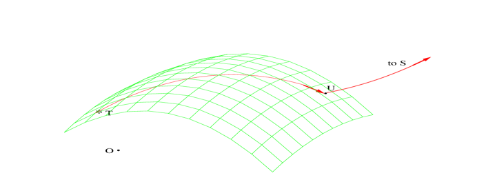
Figure 1: This cartoon shows Waleffe’s picture: a part of the boundary $\partial B$ of the basin of attraction of the point $O$ is shown. This part of the boundary coincides with the stable manifold of the equilibrium point $U$. Orbits starting near $O$ but on $\partial B$ are attracted toward $U$. Those starting near $O$ but slightly above $\partial B$ are attracted first toward $U$ but are then captured by the unstable manifold of the latter and carried away (toward turbulence). An example is the orbit through the threshold point $T$.

3 The model W97

This is a four-dimensional model which may be written

$$\dot{x}_{1}=-\delta r_{1}x_{1}+\sigma_{1}x_{4}^{2}-\sigma_{2}x_{2}x_{3},$$ (2)

$$\dot{x}_{2}=-\delta r_{2}x_{2}+\sigma_{2}x_{3}+\sigma_{2}x_{1}x_{3}-\sigma_{4}x_{4}^{2},$$ (3)

$$\dot{x}_{3}=-\delta r_{3}x_{3}+\sigma_{3}x_{4}^{2},$$ (4)

$$\dot{x}_{4}=-\left(\sigma_{1}+\delta r_{4}\right)x_{4}+x_{4}\left(\sigma_{4}x_{2}-\sigma_{1}x_{1}-\sigma_{3}x_{3}\right).$$ (5)

Here $\delta=1/R$ where $R$ is the Reynolds number and the eight constants $r_{1}$ through $\sigma_{4}$ are all positive . There are standard values for these constants (cf. [9]) that we use in this section.

This system conforms to the rules (1) and (2) of model-building. It possesses the symmetry $S=\mbox{diag}(1,1,1,-1)$ so a solution $x(t)$ has a companion solution $\tilde{x}(t)$ obtained by reversing the sign of $x_{4}(t)$ so the plane $x_{4}=0$ is an invariant plane. For these reasons there is no loss of generality in considering only solutions for which $x_{4}(t)\geq 0$. It is not difficult to show that the invariant plane $x_{4}=0$ lies entirely in $B$, the basin of attraction of the origin.

When one seeks equilibrium solutions other than the origin, they are found in pairs provided $\delta<\delta_{sn}$ or $R>R_{sn}$. The one lying closer in norm to the origin is called the“lower branch” equilibrium solution $X_{lb}$, the one lying farther away is called the “upper branch” $X_{ub}$ (see Figure 2). The lower-branch solution is unstable, with a one-dimensional unstable manifold and a three dimensional stable manifold; the upper-branch solution may be stable or unstable, depending on the choices of $R$ and of the other parameters. For the values of $R$ considered in this paper and for the standard values of the other parameters, $X_{ub}$ is asympotically stable. These equilibrium solutions are illustrated in Figure 2.

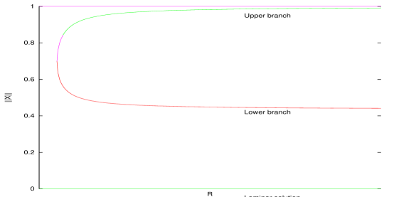
Figure 2: This is the diagram for equilibrium figures in Waleffe’s model. The lower edge, where the norm $\|X\|=0$, represents the laminar solution. The “lower branch” of further equilibrium solutions does not approach the laminar solution as $R\to\infty$ but instead tends to the indicated asymptote. However, as shown in [2], the curve of threshold values does approach the laminar solution, like $R^{-1}$.

Figure (1) suggests that orbits starting on $\partial B$ tend toward $X_{lb}$, which mediates the transition. This will be so if the the stable manifold of $X_{lb}$ coincides with $\partial B$. This seems plausible (and has been found to be the case for some other models) but is by no means inevitable: the basin boundary and the stable manifold of $X_{lb}$ are both invariant sets for the system (5) but they are defined in different manners and need not be identical. In fact, we find that they are not identical for the model W97. The stable manifold of $X_{lb}$ is a proper subset of $\partial B$, so a point on $\partial B$ lying far enough from $X_{lb}$ has a different evolution.

For W97 the threshold point $T$ has been located by Cossu ([2]). We find, by following orbits starting near $T$, that they are attracted not toward $X_{lb}$ but to a periodic orbit $P$ also lying on $\partial B$. We have thus far carried out calculations for $R=145$ and $R=190$ and we display only those for $R=190$ (those for $R=145$ are similar). We exploit Cossu’s calculations to find refinements of the threshold values $T$: by repeated bisection we obtain a pair of values, $x_{o}$ and $x_{i}$ lying respectively just outside and just inside the basin of attraction $B$ and within a short distance $\epsilon$ of one another. It follows that there is a point $T$ on $\partial B$ within $\epsilon$ of either of them. We then find the structure of the basin boundary by calculating slices of it by various hyperplanes (Figures 3 and 5). We also obtain the orbit through $T$, finding the following. On taking $x_{o}$ as initial data, we find that after a transient of a few hundred units of time, the orbit is essentially periodic for many thousands of units of time, eventually spiraling into the stable, outside point $X_{ub}$; if $x_{i}$ is taken as the initial point a similar evolution is found except that at the end, the orbit tends to the laminar point $O$. Neither of these orbits comes close to $X_{lb}$. These remarks are illustrated in Figures (3), (4) and (5).

Figure 3: A slice through the basin boundary made by the hyperplane $x_{2}=T_{2},x_{3}=T_{3}$, where $T_{i},i=1,\ldots,4$ are the components of the threshold point $T$. The parts of this region lying in $B$ are so marked; the remainder lies outside. An orbit starting very near $T$ spends a very long time hovering near a periodic orbit, indicated in projection onto this hyperplane (the transient leading from $T$ to this orbit is not shown). The complementary region to the basin becomes very narrow near $T$ but is easily resolvable numerically for these values of the parameters. .

Figure 4: A global view of the preceding figure, showing more of the nature of the basin boundary, in the same slice as in Figure (3).

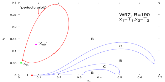
Figure 5: Like Figure (3), but a different slice.

We illustrate the results in the form of slices formed when certain two-dimensional hyperplanes intersect $\partial B$. Also seen in these diagrams are projections of the periodic orbit – and other features – onto the hyperplanes in question. The projections are indicated by placing single quotation marks around their labels.

While the self-sustaining process may be only slightly modified by replacing the equilibrium point $X_{lb}$ with the periodic orbit $P$ as the mediator of transition, the question of what role $X_{lb}$ plays in the dynamics now arises. We next turn to this.

4 Orbits starting near the point $X_{lb}$

The three-dimensional stable manifold of $X_{lb}$ coincides locally with $\partial B$. Denote by $\xi_{t}$ a unit vector transverse to $\partial B$ (for example, $\xi_{t}$ could have the unstable direction at $X_{lb}$). Then if for a scalar $v$ we choose initial data

$$x(0)=X_{lb}+v\xi_{t}$$ (6)

for a small value of $|v|$, we expect the orbit to depart from $X_{lb}$ along its unstable manifold. We anticipate that for one sign of $v$ the orbit will lie inside $B$ and for the other outside, and therefore that for one sign the orbit will tend to the origin and for the other will remain permanently outside the basin boundary, presumably tending for large $t$ to the stable equilibrium point at $X_{ub}$.

Instead, we find that all orbits tend to $O$, apparently echoing the persistent relaminarization found in other models ([4]). This is illustrated in Figure (6).

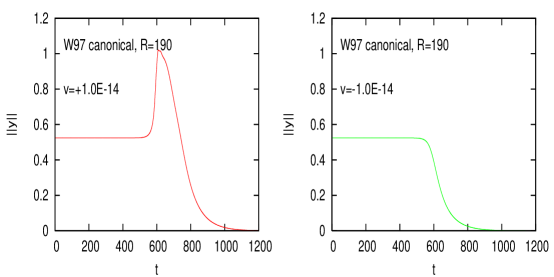
Figure 6: The model is W97 with the canonical values for the constants $r_{1}$ through $\sigma_{4}$ and $R=190$. The norms of orbits are shown on the interval [0,1200] and $v=\pm 10^{-14}$. They differ in the nature of the orbits and in the time for relaminarization to occur.

This violation of expectations could be explained by the following conjecture for the system W97 near the unstable equilibrium point $X_{lb}$: $X_{lb}$ indeed lies on $\partial B$ but, near the part of $\partial B$ on which it lies, there is a second leaf of $\partial B$ exquisitely close to the first, and it’s only for initial data in the narrow gap between the two leaves that orbits remain bounded away from the origin . If this “gap conjecture” is correct for W97 with the standard choice of parameters, the space between the two leaves is too small to be detected in the usual double precision arithmetic. The strategy we adopt below for testing this conjecture is the following.

If we put all the positive constants in W97 equal to unity we find qualitative similarity to the case with standard values. In particular, all perturbations of $X_{lb}$ relaminarize. The strategy will be to take all coefficients equal to unity with the exception of $\sigma_{1}$. An asymptotic analysis like that of [9] shows that, for small $\delta=1/R$, the lower and upper branch equilibrium points are

$$X_{lb}\approx(-\frac{\sigma_{1}^{2}}{1+\sigma_{1}^{2}},\frac{\sigma_{1}}{1+\sigma_{1}^{2}},\sigma_{1}\delta,\sigma_{1}^{1/2}\delta)$$

and

$$X_{ub}\approx(-1+2\delta,\delta^{1/2},\delta^{1/2},\delta^{3/4}).$$

For small values of $\sigma_{1}$, we find numerically that there is a large and easily detectable gap near $X_{lb}$. We then consider successively larger values of $\sigma_{1}$ to see if this gap gets successively narrower and ultimately becomes undetectable. In Figures 7 and 8, we show only slices of the basin boundary with the hyperplane $x_{2}=X_{lb2},x_{3}=X_{lb3}$ since these seem to reveal the gap most clearly. The value of $R$ is held fixed at $15$.

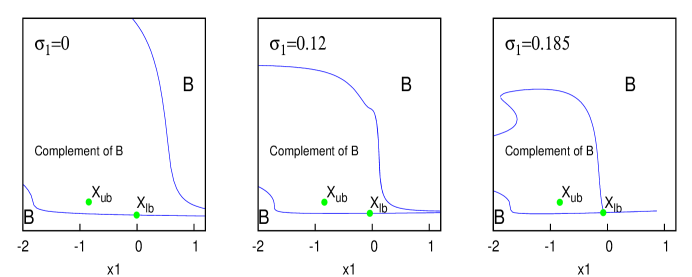
Figure 7: The ordinate is $x_{4}$. For each value of $\sigma_{1}$ shown, there is a progressively narrower gap to the right of $X_{lb}$. Orbits starting above the narrower gap require longer to relaminarize than those starting below. It looks on this scale as if the gap closes when $\sigma_{1}=0.185$, with $X_{lb}$ falling on a critical point. A close up of the region near $X_{lb}$ would show that this has not yet occurred, but see Figure 8.

These diagrams seem to confirm the gap conjecture but reveal a further, unexpected feature: there appears to be a topological change in the nature of the basin boundary for precisely the parameter value at which the gap becomes suddenly undetectable. We comment further on this in the discussion section below.

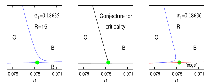
Figure 8: The large dots represent $X_{lb}$. These are closeup views of the part of phase space near $X_{lb}$. The region marked $C$ is the complement of $B$. The first and third of these diagrams are calculated but the central diagram is conjectural. The curve marked ’edge’ in the third diagram divides long-time relaminarizations from short-time relaminarizations: no points of the complementary region are detectable in the region of phase space immediately adjacent to this edge.

5 Discussion

In the self-sustaining scenario for the NS equations, the streaky flow is represented by a steady-state solution (or by a traveling-wave solution: steady in a moving frame). These have been sought and studied in some detail in the context of the NS equations ([6],[11]). The analog in W97 is the lower-branch equilibrium point $X_{lb}$. For standard values of the parameters of W97 we find that all orbits beginning near $X_{lb}$ relaminarize, whereas in a different part of phase space – nearer to the threshold point – there is a large region wherein orbits are permanently bounded away from the origin: the low-dimensional analog of persistent turbulence. Looking for this large region by beginning near $X_{lb}$ would be counter-productive, and it is possible that the analogous conclusion holds for numerical studies of the NS equations (cf. the recent exploration of ’relative periodic orbits’ [3] in the NS context).

The apparent collapse of the complementary set to the basin of attraction, as depicted in Figure (8), is reminiscent of the ’edge of chaos’ as described in ([7]) in that the line marked ’edge’ is determined in a similar manner: there is a sharp difference in relaminarization time for points just above and just below this line. It suggests a picture like that of Figure (9), wherein the ’edge’ in fact consists of two leaves of the basin boundary so close together as to be numerically indistinguishable.

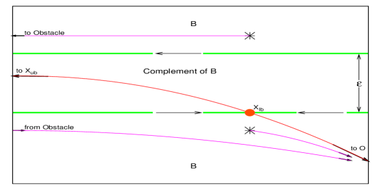
Figure 9: A conjecture regarding the ’edge.’ The distance $\epsilon$ separating the top and bottom leaves of the basin boundary is so small as to escape numerical detection. If a point could be located between these leaves, it would ultimately be captured by the stable equilibrium point $X_{ub}$ and therefore be permanently bounded away from the origin. Attempts to locate such a point are frustrated by the narrowness of the gap, and will result instead in initial points indicated by the asterisks above and below. The orbit starting above is complicated but, since it is in $B$, ultimately decays to $O$. The orbit starting below decays more directly, and more quickly, to $O$.

The diagram shown envisions a region of phase space close to $X_{lb}$ but that is because we have concentrated on this point. There are undoubtedly parts of phase space farther from $X_{lb}$ where such narrow gaps occur, with behavior that is qualitatively similar but for which the transient relaminarizations may be quantitatively quite different.

We tentatively propose the structure shown in this diagram as a building block for the edge of chaos as described elsewhere for other models (cf. [7]). This interpretation would require a repeated folding and refolding of the basin boundary of exquisite tightness, each folding modeled by such a building block. That intricate folds are possible for the basin boundaries of this and related systems is plausible not only on the basis of the pictures shown here but also experience with other model systems (e.g., [7]). It has been argued that this ’edge’ is itself a new kind of invariant set but it seems difficult to make this statement mathematically precise. In our proposed picture, the edge is from any numerical standpoint effectively invariant since orbits are as close as numerically possible to the basin boundary, which is indeed invariant.

A number of issues for further study come to mind in view of the outcomes of the work reported here. We list a few:

• What is the nature of the singularity indicated in Figure (9)? It is possible in principle that the singularity is an artifact of viewing the surface $\partial B$ through hyperplane slices and therefore does not represent any singularity of $\partial B$. Against this is the (apparent) fact that the equilibrium point $X_{lb}$ of the vector field $f(x)=Ax+b(x)$ lies at the singularity – an unlikely coincidence.

• Can we exploit the picture presented here to locate regions of phase space where there is no relaminarization? One could do that in the context of the present model by following a long-time, relaminarization orbit, choosing a point on it which is safely far from both $X_{lb}$ and from $O$, and conducting a search for $\partial B$ near this point.

• The structure of the basin boundaries makes it clear that whether a perturbation lies in $B$ or its complement depends not only on the amplitude of the perturbation but also – sensitively – on its direction in phase space. Moreover, even for perturbations in the right direction to leave $B$, a large amplitude is not necessarily more effective than a smaller one.

I wish to thank Carlo Cossu for generously sharing his data with me.

References

- [1] J.S. Bagget and L.N. Trefethen. Low-dimensional models of transition to turbulence. Phys. Fluids, 9:1043–1053, 1997.
- [2] C. Cossu. An optimality condition on the minimum energy threshold in subcritical instabilities. Comptes Rendus, 333:331–336, 2005.
- [3] Y. Duguet, C.C.T. Pringle, and R.R. Kerswell. Relative periodic orbits in transitional pipe flow. Phys. Fluids, 20:114102, 2008.
- [4] B. Eckhardt. Turbulence transition in pipe flow: some open questions. Nonlinearity, 21:T1–T11, 2008.
- [5] B. Eckhardt and A. Mersmann. Transition to turbulence in shear flow. Phys. Rev. E, 60(1):509–517, 1999.
- [6] H. Faisst and B. Eckhardt. Traveling waves in pipe flow. Phys. Rev. Lett., 91:224502, 2003.
- [7] J.D. Skufca, J.A. Yorke, and B. Eckhardt. Edge of chaos in a parallel shear flow. Phys. Rev. Lett., 96:174101–1,174101–4, 2006.
- [8] F. Waleffe. Hydrodynamic stability and turbulence: Beyond transients to a self-sustaining process. Stud. Appl. Math., 95:319, 1995.
- [9] F. Waleffe. On a self-sustaining process in shear flows. Phys. Fluids, 9(4):883–900, 1997.
- [10] F Waleffe and J. Wang. Transition threshold and the self-sustaining process. In T. Mullin and R. Kerswell, editors, IUTAM Symposium on Laminar-Turbulent Transition and Finite Amplitude Solutions, pages 85–106. Springer, 2005.
- [11] H. Wedin and R.R. Kerswell. Exact coherent structures in pipe flow: traveling wave solutions. JFM, 508:333–371, 2004.