Solitons and solitary vortices in “pancake”-shaped Bose-Einstein condensates

Abstract

We study fundamental and vortical solitons in disk-morphed Bose-Einstein condensates (BECs) subject to strong confinement along the axial direction. Starting from the three-dimensional (3D) Gross-Pitaevskii equation (GPE), we proceed to an effective 2D nonpolynomial Schrödinger equation (NPSE) derived by means of the integration over the axial coordinate. Results produced by the latter equation are in very good agreement with those obtained from the full 3D GPE, including cases when the formal 2D equation with the cubic nonlinearity is unreliable. The 2D NPSE is used to predict the density profiles and dynamical stability of repulsive and attractive BECs with zero and finite topological charge in various planar trapping configurations, including the axisymmetric harmonic confinement and 1D periodic potential. In particular, we find a stable dynamical regime that was not reported before, viz., periodic splitting and recombination of trapped vortices with topological charge $2$ or $3$ in the self-attractive BEC.

I Introduction

A natural setting for the creation of localized states, both fundamental ones and those carrying intrinsic vorticity, in Bose-Einstein condensates (BECs) is provided by “pancake” configurations, which are strongly confined in one (axial) direction, $z$, being weakly trapped in the transverse plane, ($x,y$). In the experiment, “pancakes” were created by a superposition of a tight flat optical trap, formed by a pair of strongly repulsive (blue-detuned) light sheets, and a loose in-plane radial magnetic trap Ketterle . Alternatively, the axial trap may be represented by one cell of a very strong optical lattice (OL) Hulet .

The pancake configuration may exist with either sign of the intrinsic nonlinearity, self-repulsive or self-attractive (although, as far as we know, in the latter case experiments were not reported, as yet, in the pancake geometry). In particular, the attractive sign can be induced by means of the Feshbach-resonance technique, as in well-known works which demonstrated the creation of effectively one-dimensional (1D) solitons in the condensates of ⁷Li soliton and ⁸⁵Rb soliton2 atoms, and in other settings (for instance, in experiments with the condensate formed by weakly interacting ³⁹K atoms Inguscio ). Depending on the sign of the nonlinearity, one may expect the establishment of different matter-wave patterns. In the case of the repulsion, a relatively weak (in comparison with the tight axial trap) in-plane parabolic (alias harmonic) confining potential gives rise to an axisymmetric ground state, that may be described by means of the Thomas-Fermi (TF) approximation BEC . Imparting the angular moment to the confined axisymmetric state creates a vortex, which may be unstable against the bending of its axis in the full 3D geometry bending , but is stable in the planar form. On the other hand, multiple vortices, with topological charge $S\geq 2$, were demonstrated experimentally double-vort-exper and theoretically double-vort to be unstable against splitting into unitary ones. Nevertheless, it was predicted that multiple vortices may be stabilized by imposing an anharmonic in-plane trapping potential multiple .

In the case of the self-attractive nonlinearity, a challenging problem is to predict, and create in an experiment, 2D solitons and solitary vortices (solitons with the embedded vorticity) that would be stable in the pancake setting, despite the possibility of the collapse. If the in-plane confinement is provided by the axisymmetric parabolic potential, soliton-like states are stable provided that their norm (the total number of atoms) falls below a critical value which stipulates the onset of the collapse Dodd . The critical value strongly increases for vortex solitons, but they are vulnerable, below the collapse threshold, to another instability, which tends to break them into a few fragments shaped as fundamental solitons, which may later suffer the intrinsic collapse. Stability limits for the trapped vortices in the self-attractive BEC have been studied in detail theoretically, both for the nearly planar and full 3D geometries Sadhan -DumDum2 , including the limit case of the cigar-shaped (prolate) trap, opposite to that of the oblate “pancake” Luca ; we-vortex-in-tube . In particular, it was found that such solitons with multiple charges, $S\geq 2$, are always unstable; as concerns the unitary vortices ($S=1$), they feature a region of a semi-stability between fully stable and unstable configurations, where the vortex periodically splits and recombines DumDum ; DumDum2 .

Another general possibility to stabilize both fundamental solitons and various solitary-vortex states in the 2D geometry is offered by the use of periodic (rather than parabolic) in-plane potentials, that may be typically created by means of OLs. For 2D periodic potentials, this possibility was first demonstrated in Refs. BBB1 and Yang . Then, it was shown that a quasi-1D potential, induced by a 1D OL (i.e., a periodic potential that depends on a single in-plane coordinate) can also stabilize fundamental solitons BBB2 . The general case of an anisotropic potential, composed by two perpendicular sublattices with unequal strengths, was investigated recently Thawatchai .

A very accurate model for the description of the mean-field dynamics of dilute condensates is provided by the 3D Gross-Pitaevskii equation (GPE) BEC . An effective 2D equation for the “pancake” geometry should be derived from the 3D GPE by means of an adequate reduction procedure. It was developed, using the ansatz which assumes the factorization of the wave function in the axial direction and perpendicular (pancake’s) plane, in Ref. sala-npse (see also Ref. Delgado ). The result is a nonpolynomial nonlinear Schrödinger equation(NPSE) (it takes a different nonpolynomial form in the cigar-shaped setting, when the dimension is reduced from 3 to 1 sala-npse -we-twocomp ). The objective of the present work is to use the 2D NPSE for the systematic analysis of effectively 2D localized states in both cases of the self-repulsive and self-attractive nonlinearity. To this end, we briefly recapitulate the derivation of the effective 2D equation in Section II, where the respective TF approximation is considered too. In Section III we focus on the model with the repulsive nonlinearity. Using the 2D NPSE, we construct solution families for both the ground state and vortices trapped in the axisymmetric in-plane parabolic potential. The comparison with direct numerical solutions of the underlying 3D GPE demonstrates that the effective equation, unlike the formal 2D version of the GPE, with the cubic nonlinearity, provides for virtually exact shapes of both the ground and vortex states. In Section IV, we consider the model with the self-attraction. First, we construct families of fundamental and vortical states trapped in the axisymmetric parabolic potential. In that case too, we conclude that the respective version of the 2D NPSE provides for a virtually exact prediction of the shape of the states. The 2D NPSE reproduces earlier known results for the stability of trapped states with vorticity $S=1$, and generates a new stable regime for $S=2$ and $3$, in the form of periodic splitting of the double or triple vortex into a pair or triplet of unitary vortices followed by their recombination back into the single double or triple vortex. Then, we consider the quasi-1D periodic potential, for which families of fundamental solitons are found as numerical solutions of the 2D NPSE, and also by means of the variational approximation (VA) applied directly to the underlying 3D GPE.

II The effective 2D equation

II.1 The general case

We consider the condensate formed by a large number $N$ of bosonic atoms of mass $m$ tightly trapped in axial direction $z$ by the harmonic potential, $(m/2)\omega_{z}^{2}z^{2}$, and loosely confined in transverse plane $(x,y)$ by a generic potential, $W(x,y)$. The scaled 3D GPE, which governs the mean-field dynamics of the dilute potential at zero temperature, is

$$i{\frac{\partial}{\partial t}}\Psi=\left[-{\frac{1}{2}}\nabla^{2}+V(x,y,z)+2\pi g|\Psi|^{2}\right]\Psi\;,$$ (1)

where $V(x,y,z)\equiv W(x,y)+z^{2}/2$, $g\equiv 2Na_{s}/a_{z}$ is the interaction strength, with $a_{s}$ the inter-atomic scattering length and $a_{z}=\sqrt{\hbar/(m\omega_{z})}$ the scale of the axial trapping, and 3D wave function $\Psi(\mathbf{r},t)$ is subject to normalization

$$\int|\Psi(\mathbf{r},t)|^{2}\ d^{3}\mathbf{r}=1.$$ (2)

Following Ref. sala-npse , the solution to Eq. (1) can be simplified by setting

$$\Psi(\mathbf{r},t)=\Phi(x,y,t)\ \Xi(z;\eta),$$ (3)

where $\Phi(x,y,t)$ is an arbitrary transverse wave function, and $\Xi(z,\eta)$ is its normalized axial counterpart,

$$\Xi(z;\eta)=\left(\pi\eta^{2}\right)^{-1/4}\exp{\left[-{z^{2}/}\left(2\eta^{2}\right)\right]},~{}\int_{-\infty}^{+\infty}\Xi^{2}(z)dz=1.$$ (4)

With regard to underlying condition (2), the factorization ansatz based on Eqs. (3) and (4) yield the normalization condition for the 2D wave function, $\int\int|\Phi(x,y,t)|^{2}\ dxdy=1$. In these expressions, axial width $\eta$ may depend on transverse coordinates $(x,y)$ and time $t$.

The substitution of factorized expression (3) in Eq. (1) and subsequent averaging in axial coordinate $z$ lead to the following 2D NPSE sala-npse ,

$$i{\frac{\partial}{\partial t}}\Phi=\left[-{\frac{1}{2}}\nabla_{\bot}^{2}+W(x,y)+\gamma{\frac{|\Phi|^{2}}{\eta}}+{\frac{1}{4}}\left({\frac{1}{\eta^{2}}}+\eta^{2}\right)\right]\Phi,$$ (5)

where the scaled interaction strength is

$$\gamma=2\sqrt{2\pi}Na_{s}/a_{z}\equiv\sqrt{2\pi}g,$$ (6)

and the axial width is determined by an algebraic equation,

$$\eta^{4}=1+\gamma|\Phi|^{2}\eta.$$ (7)

Exact solutions to Eq. (7) are given by the Cardano formula,

$$\eta=\pm{\frac{1}{2}}\sqrt{\frac{A^{2}-12}{3A}}+{\frac{1}{2}}\sqrt{-{\frac{A^{2}-12}{3A}}\pm 2\gamma|\Phi|^{2}\left(\frac{A^{2}-12}{3A}\right)^{-1/2}}\;,$$ (8)

where the upper and lower signs correspond, respectively, to $\gamma>0$ and $\gamma<0$, and

$$A\equiv\left({3/2}\right)^{1/3}\left(9\gamma^{2}|\Phi|^{4}+\sqrt{3}\sqrt{256+27\gamma^{4}|\Phi|^{8}}\right)^{1/3}.$$ (9)

The dependence of $\eta$ on product $\gamma|\Phi|^{2},$ as produced by Eqs. (8) and (9), is displayed in Fig. 1.

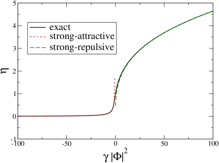
Figure 1: (Color online). Axial width $\eta$ of the pancake-shaped condensate as a function of the interaction-strength$\times$density product, $\gamma|\Phi|^{2}$. The solid curve: the full dependence following from Eq. (8); dashed and dotted curves: asymptotic expressions (12), in the cases of repulsion, $\gamma>0$, and attraction, $\gamma<0$ (except for the narrow vicinity of $\gamma|\Phi|^{2}=0$, the asymptotic curves are virtually identical to the full one, in the regions of $\gamma|\Phi|^{2}>0$ and $\gamma|\Phi|^{2}<0$, respectively).

II.2 Low- and high-density limits

In the low-density limit, $|\gamma||\Phi|^{2}\ll 1$, Eq. (7) yields a simple solution,

$$\eta_{\mathrm{low}}\approx 1+\gamma|\Phi|^{2}/4\text{.}$$ (10)

The substitution of this approximation in Eq. (5) reduces it to the nonlinear Schrödinger equation (NPSE) with the cubic-quintic (CQ) nonlinearity, in which the quintic term always corresponds to the effective self-attraction:

$$i{\frac{\partial}{\partial t}}\Phi=\left[-{\frac{1}{2}}\nabla_{\bot}^{2}+W(x,y)+\gamma|\Phi|^{2}-{\frac{3}{16}}\gamma^{2}|\Phi|^{4}\right]\Phi.$$ (11)

The derivation of the effective 1D equation from the 3D GPE in the low-density limit also leads to the NPSE with the CQ nonlinearity of the same type 1D . Note that the self-focusing quintic term in the 2D NPSE leads to the supercritical collapse (the one with zero threshold). If the 2D equation includes both quintic and cubic self-attraction terms, then a periodic potential, accounted for by $W(x,y)$ in Eq. (11), can stabilize various types of solitons and localized vortices against the (supercritical) collapse Radik . However, the 2D equation with the quintic nonlinearity only, see Eq. (14) below, cannot give rise to stable solitons, irrespective of the presence of the periodic potential Radik .

In the high-density limit, $|\gamma||\Phi|^{2}\gg 1$, asymptotic expressions for the axial width which follow from Eq. (7) are different in the cases of repulsion ($\gamma>0$) and attraction ($\gamma<0$),

$$\eta_{\mathrm{high}}^{\mathrm{(rep)}}\approx(\gamma|\phi|^{2})^{1/3},\,\eta_{\mathrm{high}}^{\mathrm{(attr)}}=-\left(\gamma\left|\Phi\right|^{2}\right)^{-1}.$$ (12)

The substitution of these approximations in Eq. (5) leads to two different 2D NPSEs: in the case of the repulsion, it is

$$i{\frac{\partial}{\partial t}}\Phi=\left[-{\frac{1}{2}}\nabla_{\bot}^{2}+W(x,y)+{\frac{5}{4}}\gamma^{2/3}|\Phi|^{4/3}\right]\Phi,$$ (13)

which coincides with the equation of the hydrodynamic type for the degenerate fermion gas in the weak-coupling regime SKA , and in the case of the attraction, the effective equation is the NPSE with the quintic term only:

$$i{\frac{\partial}{\partial t}}\Phi=\left[-{\frac{1}{2}}\left({\frac{\partial^{2}}{\partial x^{2}}}+{\frac{\partial^{2}}{\partial y^{2}}}\right)+W(x,y)-\frac{3}{4}\gamma^{2}\left|\Phi\right|^{4}\right]\Phi.$$ (14)

II.3 The Thomas-Fermi approximation

The substitution of $\Phi(x,y,t)=\phi(x,y)\ e^{-i\bar{\mu}t},$ with chemical potential $\bar{\mu}$, casts Eq. (5) in the stationary form,

$$\left[-{\frac{1}{2}}\nabla_{\bot}^{2}+{\frac{\gamma|\phi|^{2}}{\eta}}+{\frac{1}{4}}\left({\frac{1}{\eta^{2}}}+\eta^{2}\right)\right]\phi=\mu(x,y)\phi,$$ (15)

where $\mu(x,y)\equiv\bar{\mu}-W(x,y)\;$is the local chemical potential. In the Thomas-Fermi (TF) approximation, that may be relevant in the case of the repulsive interactions, i.e., $\gamma>0$, one neglects the spatial derivatives in Eq. (15), and, taking into regard Eq. (8), obtains the following expression,

$$|\phi(x,y)|^{2}={\frac{{\frac{4}{25}}\left\{\sqrt{\left[\mu(x,y)\right]^{2}+{\frac{15}{4}}}+\mu(x,y)\right\}^{2}-1}{\gamma\sqrt{\frac{2}{5}\left\{\sqrt{\left[\mu(x,y)\right]^{2}+{\frac{15}{4}}}+\mu(x,y)\right\}}}},$$ (16)

which is valid as long as it yields $|\phi(x,y)|^{2}>0$. In the region where expression (16) is negative, it is replaced by $|\phi(x,y)|^{2}\equiv 0$. In the case of $\left|\mu\left(x,y\right)-1/2\right|\ll 1/2$, the TF approximation corresponds to the low-density limit (10), with $|\phi(x,y)|^{2}\approx\gamma^{-1}\left[\mu(x,y)-{1/2}\right].$ The high-density limit (12) corresponds to large $\mu$, which yields $|\phi(x,y)|^{2}\approx{\gamma}^{-1}\left[\left(4/5\right)\mu(x,y)\right]^{3/2}.$

III The ground state and vortices in the 2D parabolic trap, with the repulsive nonlinearity

We start the analysis of trapped states, predicted by the 2D NPSE, with the case of the repulsion, assuming that the potential inside the “pancake” is also a parabolic trap (which is much weaker than the underlying axial trapping potential, $z^{2}/2$), i.e.,

$$W(x,y)={(\lambda}^{2}{/2)}(x^{2}+y^{2})$$ (17)

in Eqs. (5) and (15), with small $\lambda$. For comparison of localized states predicted by stationary NPSE (15), and by the full 3D GPE, we introduce the radial and axial probability densities, defined in terms of the 3D wave function, which is subject to normalization (2):

$$\rho_{\mathrm{3D}}(r,t)=\int_{-\infty}^{+\infty}|\Psi(\mathbf{r},t)|^{2}\ dz,~{}\rho_{\mathrm{3D}}(z,t)=2\pi\int_{0}^{\infty}|\Psi(\mathbf{r},t)|^{2}rdr,$$ (18)

where $r\equiv\sqrt{x^{2}+y^{2}}$. In the framework of the 2D description, the factorized ansatz based on Eqs. (3) and (4) yields

$$\rho_{\mathrm{2D}}(r,t)=|\Phi(r,t)|^{2},~{}\rho_{\mathrm{2D}}(z,t)=2\sqrt{\pi}\int_{0}^{\infty}\frac{rdr}{\eta(r)}e^{-z^{2}/\eta^{2}(r)}\Phi^{2}(r).$$ (19)

In Fig. 2, we display typical examples of the radial and axial densities for the repulsive condensate in the ground state, fixing $\lambda=0.1$. The respective 3D and 2D stationary wave functions were obtained by means of the imaginary-time integration, using the finite-difference Crank-Nicolson predictor-corrector code, as elaborated in Ref. sala-numerics . The figure demonstrates that the 2D NPSE provides almost exact results, in the comparison to the full 3D equation, except for some deviation of the axial density at very large values of the interaction strength, $g=200$ and $1000$. It is worthy to note that the NPSE provides for a much better accuracy than the formal 2D GPE with the cubic nonlinearity.

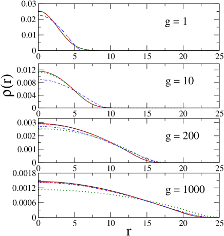
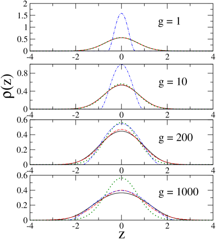
Figure 2: (Color online). Radial (a) and axial (b) probability densities, $\rho(r)$ and $\rho(z)$, for the self-repulsive condensate in the ground state trapped in parabolic potential (17) with $\lambda=0.1$. Solid, dashed, dotted, and dotted-dashed curves display the results produced, respectively, by the 3D GPE, 2D NPSE, the ordinary 2D equation with the cubic nonlinearity, and TF approximation to the 3D GPE. Values of interaction strength $g=2Na_{s}/a_{z}$ are indicated in the panels.

In the same setting, the 3D wave functions for vortex states can be sought for as $\Psi(\mathbf{r},t)=\psi(r,z,t)\ e^{iS\theta},$where $r$ and $\theta$ are the polar coordinates in the $\left(x,y\right)$ plane, $S$ is integer vorticity, and function $\psi$ obeys equation

$$i{\frac{\partial}{\partial t}}\psi = \frac{1}{2}\left[-\left({\frac{\partial^{2}}{\partial r^{2}}}+{\frac{1}{r}}{\frac{\partial}{\partial r}}+{\frac{\partial^{2}}{\partial z^{2}}}\right)+{\frac{S^{2}}{r^{2}}}\right.$$ (20)

$$\left.+\lambda^{2}r^{2}+z^{2}+4\pi g|\psi|^{2}\right]\psi\;.$$

In the case of 2D NPSE (5), the vortex corresponds to $\Phi(r,\theta,t)=\phi(r,t)e^{iS\theta},$ with Eq. (20) replaced by

$$i{\frac{\partial}{\partial t}}\phi=\frac{1}{2}\left[-\left({\frac{\partial^{2}}{\partial r^{2}}}+{\frac{1}{r}}{\frac{\partial}{\partial r}}\right)+{\frac{S^{2}}{r^{2}}}\right.$$

$$\left.+\lambda^{2}r^{2}+2\gamma{\frac{|\phi|^{2}}{\eta}}+{\frac{1}{2}}\left({\frac{1}{\eta^{2}}}+\eta^{2}\right)\right]\phi.$$ (21)

Relevant solutions to both equations () and (21) must feature the usual asymptotic form, $\left(\psi,\phi\right)\sim r^{|S|}$, at $r\rightarrow 0$.

The radial and axial profiles of the vortex states with $S=1$ are displayed in Fig. 3, for the same value of $\lambda=0.1$ as in Fig. 2. To generate these results, Eqs. (20) and (21) were also solved in the imaginary time by means of the above-mentioned finite-difference Crank-Nicolson algorithm sala-numerics . We again conclude that, as well as in the case of the ground state, the 2D NPSE produces results which, in most cases, virtually coincide with those obtained from the 3D GPE (except for some deviation of the axial profiles at very large $g$), while the formal 2D GPE with the cubic nonlinear term is essentially less accurate.

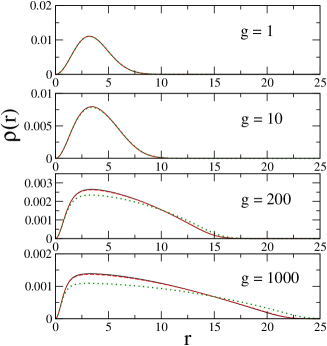
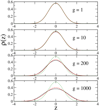
Figure 3: (Color online). The same as in Fig. 2, but for vortex states with $S=1$.

For higher values of $S$ (up to $S=3$), the radial and axial density profiles, as predicted by the 2D NPSE, are displayed, along with their counterparts for the ground state, in Fig. 4, at fixed values of the parameters,  $\lambda=0.1$ and $g=200$. As expected, the growth of $S$ leads to the increase of the size of the vortex’ core. On the other hand, the axial density profile, $\rho(z)$, is not strongly affected by the change of $S$.

We have checked that, as well as in the case of full 3D GPE with the repulsive nonlinearity and its 2D counterpart, multiple trapped vortices are unstable against splitting into solitary vortices within the framework of the 2D NPSE. This finding is not surprising, as the latter equation is derived from the 3D GPE, hence it should inherit basic properties of solutions of the 3D equation.

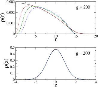
Figure 4: (Color online). The upper and lower panels display, respectively, the radial and axial probability densities, $\rho(r)$ and $\rho(z)$, for the ground state and higher-order vortices, as found from the 2D NPSE with $\lambda=0.1$ and $g\equiv 2Na_{s}/a_{z}=200$. The solid, dotted, dashed, and dotted-dashed curves pertain, respectively, to $S=0$, $S=1$, $S=2$, and $S=3$ (all vortices with $S\geq 2$ are unstable against splitting into unitary vortices).

IV Solitons and solitary vortices in the case of the attractive nonlinearity

IV.1 The axisymmetric parabolic trap

In the case of the attractive nonlinearity, $g<0$, localized states and vortices supported by the in-plane potential – in particular, axisymmetric parabolic potential (17) – may be considered as solitons Dodd -we-vortex-in-tube . In Fig. 5 we display the radial and axial profiles of the solitons found from the NPSE with potential (17), for $\lambda=0.1$ and $g=-1$. It can be checked that, for sufficiently small values of $|g|$, at which the collapse does  not take place, the full 3D GPE yields virtually the same profiles.

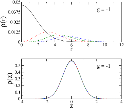
Figure 5: (Color online). The same as in Fig. 4 (again, with $\lambda=0.1$), but for the self-attractive condensate, with nonlinearity strength $g\equiv 2Na_{s}/a_{z}=-1$.

Under normalization conditions (2) and parabolic confinement (17), the critical value, $g_{c}$, of the interaction strength for the onset of collapse can be found as that at which the stationary soliton solution disappears. These values, as found from the set of the three models (3D GPE, 2D NPSE, and the formal 2D GPE, with $\lambda=0.1$), are collected in Table 1, for different values of vorticity $S$. Naturally, $g_{c}$ quickly increases with $S$ DumDum , and we once again conclude that the NPSE provides for high accuracy, especially in comparison with the large error in the predictions produced by the formal 2D equation with the attractive cubic nonlinearity.

$S$	$\left(~{}g_{c}\right)_{\mathrm{3D-GPE}}$	$\left(g_{c}\right)_{\mathrm{2D-NPSE}}$	$\left(g_{c}\right)_{\mathrm{2D-GPE}}$
$0$	$-1.9$	$-1.9$	$-2.3$
$1$	$-7.3$	$-7.2$	$-8.9$
$2$	$-12.4$	$-12.3$	$-15.8$
$3$	$-16.9$	$-16.8$	$-21.6$

Table 1. Critical strength $g_{c}$ for the onset of the collapse in the attractive condensate with vorticity $S$, confined by in-plane potential (17) with $\lambda=0.1$. The table compares the predictions produced by the full 3D GPE, the effective 2D equation (NPSE), and the formal 2D equation (GPE) with the cubic nonlinearity.

An important issue is the stability of solitary vortices with vorticity $S$ in the axisymmetric harmonic trap. We tackled this problem by means of direct simulations of the time-dependent 2D NPSE, Eq. (5), using a finite-difference real-time Crank-Nicolson algorithm sala-numerics . The initial conditions were taken as

$$\Phi(x,y,t=0)=C\ (x+iy)^{S}\ \exp\left[-\frac{\lambda}{2}\left(x^{2}+\frac{y^{2}}{\delta^{2}}\right)\right],$$ (22)

where $C$ is a normalization constant, and $\delta\neq 1$ accounts for possible breakup of the axial symmetry of the vortex, i.e., an initial perturbation applied to the vortex. Note that, with $\delta=1$, Eq. (22) gives the exact quantum-mechanical wave function of the stationary vortex configuration (for $g=0$).

We report results of the simulations for $\delta=1.1$ and trap’s strength $\lambda=0.1$. We have concluded that the trapped vortex with $S=1$ is stable for $g>-1.3$: in this region, the initial perturbation leads only to intrinsic periodic oscillations of the vortex, which maintains its integrity. In agreement with previously published results Ueda -DumDum2 , the value of the nonlinearity strength at the stability border, $g_{\mathrm{stab}}=-1.3$, is much lower than at the collapse threshold, $g_{c}=-7.2$.

Outside the stability domain, i.e., at $-g\geq 1.3$, we observed splitting of the trapped vortex into two solitary fragments, which would rotate and recombine back into the vortex. In the interval $1.3\leq-g<1.4$ the splitting-recombination cycle repeats itself quasi-periodically, as shown in Fig. 6, where we have plotted the planar density profile, $|\Phi(x,y,t)|^{2}$, at four instants of time corresponding to different stages of the cycle. Note that a similar dynamical regime was previously demonstrated in Refs. Ueda ; DumDum , in the framework of the ordinary 2D equation with the cubic self-attractive term. If the self-attraction is stronger, viz., $1.4\leq-g<1.5$, the two fragments suffer an intrinsic collapse after two cycles (in the case shown in Fig. 6 the collapse takes place at $t\simeq 125$). For a still stronger self-attraction, $-g\geq 1.5$, the two rotating fragments do not recombine at all, quickly undergoing the intrinsic collapse.

Figure 6: Density profiles $|\Phi(x,y,t)|^{2}$ for the solitary vortex with $S=1$ and $g=-1.4$, obtained by solving the time-dependent 2D NPSE, Eq. (5), with $\lambda=0.1$. The four snapshots correspond to $t=0$ (a), $t=56$ (b), $t=88$ (c), $t=120$ (d). Time is given in units of $1/\omega_{z}$. The figure displays the quasiperiodic process of the alternating splittings and recombinations of the vortex ending with the collapse, see the text.

We have also investigated the stability of the solitary vortex with $S=2$. In agreement with Ref. DumDum , it was found that the double vortex can never be stable against splitting into a pair of unitary ones. Nevertheless, a stable dynamical regime, which has not been reported in previous studies, was found in this case: the simulations of Eq. (5), with initial conditions (22) corresponding to $S=2$, demonstrate that, at small values of the interaction strength, $-g~{}\leq 0.5$, the double vortex periodically features incomplete separation into two vortices, which manifests itself in the splitting of the zero-amplitude point (the center of the vortex) into a pair of local minima, separated by a relatively small distance [see Figs. 7(b,d)], which is followed by recombination of the pair back into a single point, see a set of snapshots in Fig. 7.

Figure 7: The same as in Fig. 6, but for the solitary vortex with $S=2$ and $g=-0.3$. The snapshots pertain to $t=0$ (a), $t=16$ (b), $t=32$ (c), $t=48$ (d). The figure displays one-and-a-half cycles of the periodic process (of period $\tau\simeq 32$) of the alternating splittings and recombinations of the vortex, see the text.

At larger values of the interaction strength, $-g>0.5$, the switchings between the states with one and two local minima is a transient regime, which is followed by permanent splitting of the double vortex into a pair of unitary vortices rotating around point $x=y=0$, as shown in Fig. 8. Finally, at $-g\geq 1.8$ the evolution of the double vortex ends up with the collapse.

Figure 8: The same as in Fig. 7, but for $g=-0.8$. The snapshots pertain to $t=0$ (a), $t=44$ (b), $t=136$ (c), $t=168$ (d). The figure displays the permanent splitting of the double vortex into a pair of rotating unitary vortices, see the text.

For the sake of the completeness of the analysis, we have also analyzed the dynamics of the triple vortex, with $S=3$. It features a trend to the splitting into a state with three local minima of the amplitude. At small enough values of $|g|$, the splitting is periodically followed by the recombination into the original triple vortex, while at larger values of $|g|$ it permanently splits into a set of three rotating unitary vortices.

IV.2 The periodic in-plane potential

As discussed in Introduction, a problem of considerable interest is the stabilization of fundamental (non-vortical) 2D solitons in the attractive condensate loaded into a quasi-1D periodic potential, corresponding to a 1D OL (optical lattice); the same problem has another physical realization in terms of nonlinear optics BBB2 . In this section, we address the problem within the framework of NPSE (5) with potential $W(x,y)=-V_{0}\cos{(2kx)}$. Accordingly, the full potential in 3D GPE (1) is $V(x,y,z)=-V_{0}\cos{(2kx)}+z^{2}/2.$

First, the corresponding stationary solutions to the full three-dimensional GPE, Eq. (1), are looked for as $\Psi(\mathbf{r},t)=\psi(\mathbf{r})\exp(-i\mu t),$ with chemical potential $\mu$ and real function $\psi$ which obeys equation

$$\left[-\frac{1}{2}\nabla^{2}-V_{0}\cos{(2kx)}+{\frac{1}{2}}z^{2}+2\pi g|\psi|^{2}\right]\psi=\mu\psi.$$ (23)

This equation can be obtained by minimizing the energy functional,

$$E=\int d^{3}\mathbf{r}\ \psi^{\ast}\left[-{\frac{1}{2}}\nabla^{2}-V_{0}\cos{(2kx)}+{\frac{1}{2}}z^{2}\psi+\pi g|\psi|\right]^{2}\psi,$$ (24)

subject to constraint (2), which results in the following expression for the chemical potential,

$$\mu=E+\pi g\int|\psi(\mathbf{r})|^{4}d\mathbf{r}.$$ (25)

To predict solitons by means of the VA (variational approximation), we use the normalized 3D Gaussian ansatz BBB1 ,

$$\psi(\mathbf{r})={\frac{1}{\pi^{3/4}(\sigma_{1}\sigma_{2}\sigma_{3})^{1/2}}}\exp{\left\{-{\frac{x^{2}}{2\sigma_{1}^{2}}}-{\frac{y^{2}}{2\sigma_{2}^{2}}}-{\frac{z^{2}}{2\sigma_{3}^{2}}}\right\},}$$ (26)

with widths $\sigma_{1}$, $\sigma_{2}$ and $\sigma_{3}$. Inserting the ansatz into Eq. (24), one obtains

$$E={\frac{1}{4\sigma_{1}^{2}}}+{\frac{1}{4\sigma_{2}^{2}}}+{\frac{1}{4\sigma_{3}^{2}}}-V_{0}\exp{(-k^{2}\sigma_{1}^{2})}+{\frac{1}{4}}\sigma_{3}^{2}+{\frac{g}{\sqrt{2\pi}}}{\frac{1}{\sigma_{1}\sigma_{2}\sigma_{3}}},$$ (27)

and Eq. (25) yields, in the same approximation, $\mu=E+g/\left(\sqrt{2\pi}\sigma_{1}\sigma_{2}\sigma_{3}\right).$ Aiming to predict the ground state in the framework of the VA, we look for values of $\sigma_{1}$, $\sigma_{2}$, and $\sigma_{3}$ that minimize the energy, imposing conditions $\partial E/\partial{\sigma}_{1,2,3}=0$. In this way, we derive the following variational equations,

$$4V_{0}k^{2}\sigma_{1}^{4}\exp{(-k^{2}\sigma_{1}^{2})}=1+{\frac{g}{\sqrt{2\pi}}}{\frac{\sigma_{1}}{\sigma_{2}\sigma_{3}}}$$

$${\frac{1}{\sigma_{2}}}=-{\frac{g}{\sqrt{2\pi}}}{\frac{1}{\sigma_{1}\sigma_{3}},~{}}\sigma_{3}^{4}=1+{\frac{g}{\sqrt{2\pi}}}{\frac{\sigma_{3}}{\sigma_{1}\sigma_{2}}}.$$ (28)

A solution corresponds to a true minimum of the energy provided that the respective Hessian, $\partial^{2}E/\partial\sigma_{i}\partial\sigma_{j}$, is positive definite.

Analysis of the variational equations demonstrates that they may yield the ground-state solution if the OL is strong enough, viz., $V_{0}>e^{2}k^{2}/16$. Under this condition, the solutions exists for $g_{c}<g<0$, where critical strength $g_{c}$ depends on $V_{0}$ and $k$. Notice that, restricting the VA to the 2D setting, i.e., fixing $\sigma_{3}=1$, cf. Eq. (4), one will instead find stable solutions for $g_{c}<g<g_{s}$, with $g_{c}=-\sqrt{2\pi}$, and $g_{s}=-\sqrt{2\pi\left[1-16V_{0}/(e^{2}k^{2})\right]}$ for $V_{0}<e^{2}k^{2}/16$, while $g_{s}=0$ for $V_{0}>e^{2}k^{2}/16$ BBB2 . The expression for $g_{s}$ predicts the minimum absolute value of the self-attraction strength, above which the state cannot remain localized in the periodic potential (in fact, the vanishing of $g_{s}$ for $V_{0}>e^{2}k^{2}/1$ is an artifact of the VA Salerno ; BBB2 ; in the numerical solution reported for the 2D GPE with the self-attractive cubic term, $g_{s}$ never vanishes BBB1 ; Salerno ; BBB2 ).

Numerically found solutions of Eqs. (28) are plotted versus $g$ in the upper panel of Fig. 9, for $V_{0}=1$ and $k=1$ (dashed lines). We include also the corresponding widths obtained by solving the 2D NPSE. The lower panel of Fig. 9 shows critical interaction strength $g_{c}$ versus amplitude $V_{0}$ of the periodic potential. At $|g|~{}>|g_{c}|$, solutions for solitons do not exist anymore.

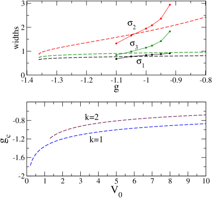
Figure 9: (Color online). In the upper panel, the dashed curves depict widths $\sigma_{1}$, $\sigma_{2}$, $\sigma_{3}$ of the soliton, in the model with the quasi-1D in-plane potential, versus self-attraction strength $g$, as predicted by the VA (variational approximation) for $V_{0}=k=1$. The solid lines with dots show the widths as found from a numerical solutions of the 2D NPSE. The lower panel displays critical interaction strength $g_{c}$ for the onset of the collapse versus amplitude $V_{0}$ of the periodic potential, as predicted by the VA, for two different values of the wavenumber of the periodic potential, $k=1$ and $k=2$.

Comparing the predictions of the VA with results produced by the 2D NPSE, we conclude that, in the case of weak nonlinearity, the VA based on the Gaussian ansatz is wrong, which is not surprising: in that case, solitons are not localized like Gaussians, but rather extend over several cells of the periodic potential Salerno ; BBB2 . In particular, similar to what was found in the 2D model with the cubic nonlinearity, and contrary to the prediction of the VA, the above-mentioned critical value $g_{s}$, below which (at $|g|~{}<\left|g_{c}\right|$) the delocalization of the 2D soliton takes place, never drops to zero, as shown in Table 2. On the other hand, critical strength $g_{c}$ for the onset of the collapse, as predicted by the VA, is indeed close to what is found from the numerical solution of the 2D NPSE, which is explained by the fact that the collapse occurs in well localized configurations. Direct simulations of the time-dependent 2D NPSE corroborate a natural expectations that the fundamental soliton is always stable in its existence range, $g_{c}<g<g_{s}$.

$V_{0}$	$g_{c}$	$g_{s}$
$1$	$-1.12$	$-0.91$
$2$	$-0.92$	$-0.43$
$3$	$-0.81$	$-0.25$

Table 2. Critical strengths $g_{c}$ and $g_{s}$ between which the fundamental soliton exists (and is stable) in the model with the quasi-1D periodic potential with amplitude $V_{0}$ and wavenumber $k=1$, as found from the numerical solution of the 2D NPSE.

Finally, typical profiles of the soliton in the present version of the model, as found from a numerical solution of Eq. (23), are shown in Fig. 10, by means of the density integrated in the free ($y$) direction, $\rho(x)=\int_{-\infty}^{+\infty}\psi^{2}\left(x,y\right)dy$. The figure corroborates that the profile indeed features a trend to delocalization with the decrease of $|g|$.

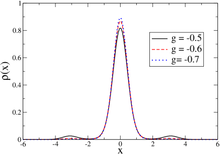
Figure 10: (Color online). Density profiles of the fundamental solitons stabilized by the quasi-1D periodic in-plane potential are shown for three values of self-attraction strength $g$, while the amplitude and wavenumber of the potential are fixed, $V_{0}=-2$ and $k=1$. The density, $\rho(x)$, is integrated in the free direction, $y$.

V Conclusion

In this work, we have reported results of the analysis of localized states in nearly-2D (“pancake”-shaped) BEC, with both signs of the intrinsic nonlinearity, repulsive and attractive. The localized states represent both the ground state, with zero vorticity, and excited states in the form of localized vortices. The main objective of the work was to apply the nonpolynomial nonlinear Schrödinger equation (NPSE) derived from the full 3D GPE (Gross-Pitaevskii equation), to the analysis of the pancake-morphed localized states. First of all, it has been demonstrated that, in the case of the self-repulsive nonlinearity and relatively weak parabolic (harmonic) in-plane axisymmetric trapping potential, the 2D NPSE predicts both the radial and axial profiles of the ground states and vortices, with the topological charge up to $S=3$, in a virtually exact form, if compared with numerical solutions of the underlying 3D GPE. On the contrary to that, the formal application of the ordinary 2D equation with the cubic nonlinearity, or Thomas-Fermi approximation derived form the 3D GPE, yields a large error. Similar conclusions have been made for the fundamental and vortical solitons in the model with the same axisymmetric trapping potential and self-attractive nonlinearity. As concerns the stability, a new result was reported for the trapped vortices with $S=2$ and $3$ in the self-attractive potential: at sufficiently small values of the nonlinearity strength, they feature a stable dynamical regime in the form of periodic splittings (respectively, into a pair or triplet of unitary vortices) and recombinations.

Finally, fundamental solitons were studied in the model combining the 1D in-plane periodic trapping potential, which does not depend on one of the planar coordinates, and the self-attractive nonlinearity. In this case, we compared predictions of the VA (variational approximation), derived for the 3D GPE, and numerical solutions of the 2D GPE. As a result, it has been concluded (as might be expected) that the VA yields reasonable results, provided that the nonlinearity is not too weak, in which case the underlying assumption of the localization of the fundamental soliton around one cell of the periodic potential is not valid.

References

- (1) A. Görlitz, J. M. Vogels, A. E. Leanhardt, C. Raman, T. L. Gustavson, J. R. Abo-Shaeer, A. P. Chikkatur, S. Gupta, S. Inouye, T. Rosenband, and W. Ketterle, Phys. Rev. Lett. 87, 130402 (2001).
- (2) J. Chen, J. G. Story, J. J. Tollet, and R. G. Hulet, Phys. Rev. Lett. 69, 1344 (1992).
- (3) K. E. Strecker, G. B. Partridge, A. G. Truscott, and R. G. Hulet, Nature 417, 150 (2002); L. Khaykovich, F. Schreck, G. Ferrari, T. Bourdel, J. Cubizolles, L. D. Carr, Y. Castin, and C. Salomon, Science 296, 1290 (2002).
- (4) S. L. Cornish, S. T. Thompson, and C. E. Wieman, Phys. Rev. Lett. 96, 170401 (2006).
- (5) G. Roati, M. Zaccanti, C. D’Errico, J. Catani, M. Modugno, A. Simoni, M. Inguscio, and G. Modugno, Phys. Rev. Lett. 99, 010403 (2007).
- (6) C. J. Pethick and H. Smith, Bose-Einstein Condensation in Dilute Gases (Cambridge University Press, 2002).
- (7) B. P. Anderson, P. C. Haljan, C. A. Regal, D. L. Feder, L. A. Collins, C. W. Clark, and E. A. Cornell, Phys. Rev. Lett. 86, 2926 (2001).
- (8) Y. Shin, M. Saba, M. Vengalattore, T. A. Pasquini, C. Sanner, A. E. Leanhardt, M. Prentiss, D. E. Pritchard, and W. Ketterle, Phys. Rev. Lett. 93, 160406 (2004).
- (9) Y. Kawaguchi and T. Ohmi, Phys. Rev. A 70, 043610 (2004); K. Gawryluk, M. Brewczyk, and K. Rzażewski, J. Phys. B: At. Mol. Opt. Phys. 39, L225 (2006); J. A. M. Huhtamäki, M. Möttönen, T. Isoshima, V. Pietilä, and S. M. M. Virtane, Phys. Rev. Lett. 97, 110406 (2006); A. Muñoz Mateo and V. Delgado, ibid. 97, 180409 (2006).
- (10) A. L. Fetter, Phys. Rev. A 64, 063608 (2001); E. Lundh, Phys. Rev. A 65, 043604 (2002); K. Kasamatsu, M. Tsubota, and M. Ueda, Phys. Rev. A 66, 053606 (2002); G. M. Kavoulakis and G. Baym, New J. Phys. 5, 51.1 (2003); A. Aftalion and I. Danaila, Phys. Rev. A 69, 033608 (2004); U. R. Fischer and G. Baym, Phys. Rev. Lett. 90, 140402 (2003); A. D. Jackson and G. M. Kavoulakis, Phys. Rev. A 70, 023601 (2004); T. K. Ghosh, ibid. 69, 043606 (2004).
- (11) F. Dalfovo and S. Stringari, Phys. Rev. A 53; 2477 (1996); R. J. Dodd, J. Res. Natl. Inst. Stand. Technol. 101, 545 (1996).
- (12) S. K. Adhikari, Phys. Rev. E 65, 016703 (2001).
- (13) H. Saito, M. Ueda, Phys. Rev. Lett. 89, 190402 (2002).
- (14) T. J. Alexander, L. Bergé, Phys. Rev. E 65, 026611 (2002).
- (15) D. Mihalache, D. Mazilu, B. A. Malomed, F. Lederer Phys. Rev. A 73, 043615 (2006).
- (16) L. D. Carr and C. W. Clark, Phys. Rev. Lett. 97, 010403 (2006).
- (17) B. A. Malomed, F. Lederer, D. Mazilu, and D. Mihalache, Phys. Lett. A 361, 336 (2007).
- (18) L. Salasnich, Laser Phys. 14, 291 (2004).
- (19) L. Salasnich, B. A. Malomed, and F. Toigo, Phys. Rev. A 76, 963614 (2007).
- (20) B. B. Baizakov, B. A. Malomed, and M. Salerno, Europhys. Lett. 63, 642-648 (2003); Phys. Rev. E 74, 066615 (2006).
- (21) J. Yang and Musslimani, Opt. Lett. 28, 2094 (2003); Z. H. Musslimani and J. Yang, J. Opt. Soc. Am. B 21, 973 (2004).
- (22) B. B. Baizakov, B. A. Malomed and M. Salerno, Phys. Rev. A 70, 053613 (2004).
- (23) T. Mayteevarunyoo, B. A. Malomed, B. B. Baizakov, and M. Salerno, Physica D, in press.
- (24) L. Salasnich, A. Parola, and L. Reatto, Phys. Rev. A 65, 043614 (2002).
- (25) A. M. Mateo and V. Delgado, Phys. Rev. A 77, 013617 (2008).
- (26) L. Salasnich and B. A. Malomed, Phys. Rev. A 74, 053610 (2006).
- (27) A. E. Muryshev, G. V. Shlyapnikov, W. Ertmer, K. Sengstock, and M. Lewenstein, Phys. Rev. Lett. 89, 110401 (2002); S. Sinha, A. Y. Cherny, D. Kovrizhin, and J. Brand, Phys. Rev. Lett. 96, 030406 (2006).
- (28) R. Driben and B. A. Malomed, Eur. Phys. J. D 50, 317 (2008).
- (29) S. Adhikari and B. A. Malomed, Europhys. Lett. 79, 50003 (2007); Physica D, in press.
- (30) E. Cerboneschi, R. Mannella, E. Arimondo, and L. Salasnich, Phys. Lett. A 249, 495 (1998); L. Salasnich, A. Parola, and L. Reatto, Phys. Rev. A 64, 023601 (2001).
- (31) B. B. Baizakov and M. Salerno, Phys. Rev. A 69, 013602 (2004).
- (32) L. Salasnich, Laser Phys. 15, 366 (2005).