A photometric study of the field around the candidate recoiling/binary black hole SDSS J092712.65+294344.0

Abstract

We present a photometric FUV to K_s-band study of the field around quasar SDSS J092712.65+294344.0. The SDSS spectrum of this object shows various emission lines with two distinct redshifts, at $z=0.699$ and $z=0.712$. Because of this peculiar spectroscopic feature this source has been proposed as a candidate recoiling or binary black hole. A third alternative model involves two galaxies moving in the centre of a rich galaxy cluster. Here we present a study addressing the possible presence of such a rich cluster of galaxies in the SDSS J092712.65+294344.0 field. We observed the $3.6\times 2.6$ square arcmin field in the K_s-band and matched the NIR data with the FUV and NUV images in the GALEX archive and the $ugriz$ observations in the SDSS. From various colour-colour diagrams we were able to classify the nature of 32 sources, only 6–11 of which have colours consistent with galaxies at $z\approx 0.7$. We compare these numbers with the surface density of galaxies, stars & quasars, and the expectations for typical galaxy clusters both at low and high redshift. Our study shows that the galaxy cluster scenario is in clear disagreement with the new observations.

1 Introduction

SDSS J092712.65+294344.0 (hereafter S0927; Adelman-McCarthy et al., 2008), is a quasar with a very peculiar spectrum. It exhibits a set of optical broad and narrow emission lines (“b-system”), blueshifted $\approx 2650$ km s^-1 with respect to a second set of narrow emission lines (“r-system”).

Recently three different models have been proposed in order to explain the peculiar spectral features of S0927. Based on the recent results of Schnittman & Buonanno (2007) and Campanelli et al. (2007), Komossa et al. (2008) suggest that S0927 is the first candidate recoiling remnant of a massive black hole (MBH) binary coalescence, ejected from the nucleus of its host galaxy by gravitational radiation recoil. In this model the (broad and narrow) b-system lines are emitted by gas comoving with the recoiling MBH, while the r-system lines are emitted by the gas in the host galaxy.

Bogdanovic, Eracleous & Sigurdsson (2009) and Dotti et al. (2009) noticed that Komossa’s model depends on an unlikely combination of parameters for the coalescing MBH binary, and has difficulty explaining the narrow emission lines of the b-system. These two papers proposed an alternative model, assuming the presence of a sub–parsec separation MBH binary in the centre of the host galaxy. In this model the blueshift of the b-system is related to the orbital motion of the MBH binary, while the r-system corresponds to the narrow line region of the host.

A third model has been discussed in Heckman et al. (2009) and Shields, Bonning & Salviander (2009). The authors consider the possibility of a chance superposition of two galaxies, assuming the presence of a rich galaxy cluster hosting S0927. The different systems of lines at different redshifts are produced in two different galaxies, moving at high relative velocity deeply inside the potential well of the cluster. This model is the simplest explanation for the three sets of lines, and is immediately testable Such a high velocity difference between the two galaxies is inconsistent with a simple on–going merger, and requires the deep potential well of a rich galaxy cluster. From the study of SDSS $ugriz$ photometry, Heckman et al. (2009) report the detection of a number ($\sim 10$) of faint, red sources within a $4\times 4$ square arcmin box around S0927, which are consistent with early-type galaxies at $z\approx 0.65$. The analysis in Heckman et al. (2009) is limited by the fact that the optical colours of red stars and of galaxies at $z=0.7$ are similar, and the latter are practically unresolved under typical SDSS seeing conditions. To improve this study, we obtained a deep NIR image of the field of S0927. Moreover, following Niemack et al. (2009) we also consider the UV information from GALEX to better assess the nature and redshift of field sources. We will then compare the number of sources found consistent with $z=0.7$ with the expectations for a galaxy cluster at that redshift.

Throughout the paper, we will adopt a concordance cosmology with $H_{0}=70$ km s^-1 Mpc^-1, $\Omega_{m}=0.3$, $\Omega_{\Lambda}=0.7$. Within this cosmology, the distance modulus at $z=0.7$ is $43.15$ mag and the angular scale is $7.15$ kpc/^′′.

2 NIR observations and data reduction

K_s-band photometry of the S0927 field was obtained using TIFKAM (Pogge et al., 1998) at the MDM Observatory 2.4m telescope on the night of 2008 November 3. The observing conditions were good with a seeing of $1.0^{\prime\prime}$ – $1.2^{\prime\prime}$ throughout. The individual exposure times were 20s, with 5 coadds per image, resulting in 100s integration time per image. The telescope was dithered using a $3\times 3$ grid to allow for accurate subtraction of the NIR background. The data were processed using standard iraf routines. The final mosaiced image, displayed in Fig. 1, was created using the xdimsum package. The total exposure time is 90 minutes.

Astrometric calibration was performed through comparison with the USNO database. The photometric zero point (ZP) was computed by comparing the instrumental magnitudes of field stars to the 2MASS catalogue (see Table 1). From the RMS of sky counts within a seeing radius, we estimate a 3-$\sigma$ limiting magnitude of $m_{\rm Ks}^{\rm limit}=19.45$.

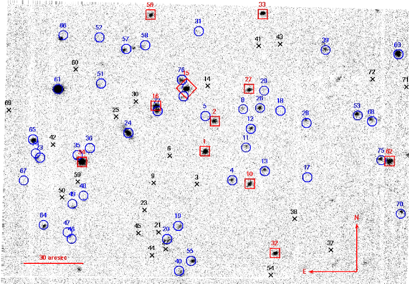
Figure 1: The K_s-band image of the field around S0927, which is labelled with n.15 (diamond). Objects labelled from 1 to 74 are present in the SDSS photometric catalogue, the others are reported here for the first time. Crosses mark the sources below our sensitivity limit in all the available images. Squares refer to the 11 objects consistent with $z\approx 0.7$ galaxies, according to our colour-colour diagnostics. All of the other sources are labelled with circles.

3 Archive data

Images of the field of S0927 are publicly available in the archives of the Galaxy Evolution Explorer (GALEX) and of the Sloan Digital Sky Survey (SDSS).

GALEX features two broad band filters at central wavelengths of $\sim 1500$Å (FUV) and $\sim 2300$Å (NUV). The field of S0927 was imaged as a part of the GALEX All Sky Survey. The point spread function (PSF) in the FUV and NUV images is $3.7^{\prime\prime}$ and $5.3^{\prime\prime}$, respectively, with a pixel scale of $1.5^{\prime\prime}$/pix. The exposure time of the two images is 112s. Assuming the zero points provided in the GALEX website (cfr Table 1), this yields a limiting magnitude of $m_{\rm FUV}^{\rm limit}=19.9$ and $m_{\rm NUV}^{\rm limit}=20.2$.

The SDSS Data Release 6 (Adelman-McCarthy et al., 2008) provides $ugriz$ photometry of nearly a quarter of the sky. The typical seeing is $\sim 1.5^{\prime\prime}$. The pixel scale is $0.396^{\prime\prime}$/pix. We estimate the photometric zero points of each band by a comparison with the instrumental magnitudes of the sources and the values reported in the SDSS catalogue. The zero points, magnitude limits and angular resolution of the available images are summarised in Table 1.

Table 1: Properties of the available images. (1): filter. (2) zero point. We list the mean and RMS values, estimated through the comparison between catalogue and instrumental magnitudes of field sources. (3) limiting magnitude due to background counts. (4) pixel scale. (5) point spread function (=seeing in ground based observations). (6) number of sources exceeding the sensitivity limit in each band.

Filter	ZP	Limit mag	Pixel scale	PSF	N.det.
	[mag]	[mag]	[′′/pix]	[′′]
(1)	(2)	(3)	(4)	(5)	(6)
FUV	$18.82$	$19.9$	$1.5$	$3.75$	3
NUV	$20.08$	$20.2$	$1.5$	$5.30$	3
$u$	$23.32\pm 0.25$	$21.24$	$0.396$	$1.18$	5
$g$	$24.17\pm 0.17$	$22.17$	$0.396$	$1.11$	22
$r$	$23.93\pm 0.09$	$21.72$	$0.396$	$1.07$	29
$i$	$23.54\pm 0.12$	$21.15$	$0.396$	$0.94$	44
$z$	$22.39\pm 0.10$	$20.07$	$0.396$	$0.94$	21
Ks	$22.98\pm 0.10$	$19.45$	$0.206$	$0.92$	47

4 Data analysis

We limit our analysis to the $3.6\times 2.6$ arcmin region around S0927 covered in all 8 bands (where the limit is provided by the region observed in the K_s-band image).

We re-measured the magnitudes of each source in all the available bands. We consider a source as detected if its flux (in counts) is larger than three times the RMS of the sky in the PSF area. The SDSS photometric catalogue lists 74 sources in our frame. Additional three sources are detected in the K_s-band but do not appear in the SDSS catalogue. As they lie close to bright companions, we argue that the SDSS source selection algorithm fails to de-blend them. The whole sample therefore consists of 77 objects.

GALEX images are the shallowest: Only 3 sources are detected in FUV and NUV, and they all appear in the images in the other bands. Six sources are detected in the SDSS but fall below our sensitivity limit in K_s. From visual inspection, we find that all of them are faint, early spectral-type stars which we miss in K_s-band due to their blue SED.

Our criterion is somewhat stricter than the SDSS detection algorithm, hence 23 sources are not detected in any of our bands. From a careful inspection, we find that ten of them are extremely faint sources ($m\mathrel{\hbox to0.0pt{\lower 3.0pt\hbox{$\sim$}\hss}\raise 2.0pt\hbox{$>$}}24$ in the SDSS photometric catalogue) and are possibly artifacts of the SDSS source detection algorithm. The remaining sources are detected with a lower significance (e.g., if we relax our threshold to 2-$\sigma$ fluctuations over the sky count RMS in the PSF area, 6 other sources are detected). In section 6.2 we will see how relaxing our sensitivity limit would affect the results of our analysis. The remaining 54 sources, detected in at least a single band, are listed in Table LABEL:tab_allsources.

We note that at $z=0.7$, 5 kpc $\approx$ $0.7^{\prime\prime}$, thus most of the light from galaxies at this redshift would be enclosed in the typical seeing of our data. This is why morphology cannot help in the identification of the nature of our sample sources: With the exception of sources n.24 and n.40, which are well-resolved foreground galaxies, all the objects are practically unresolved.

5 Classification of the observed sources

We use several colour-colour diagnostic diagrams to select possible galaxy candidates. This can be applied on a limited number of sources, because of the relative shallowness of the SDSS photometry in each particular band. Note that all our colour cuts are intended to provide a rule of thumb for distringuishing between stars and possible galaxy candidates.

We derive reference colours of galaxies and quasars by measuring the spectral magnitudes in each band from the Elliptical and Sc galaxy templates by Mannucci et al. (2001) and the quasar template by Francis et al. (1991), redshifted to $z=0.7$. We also show the locus of main sequence stars in our diagrams using the work by Girardi et al. (2005) and the prediction of TRILEGAL software as reference.

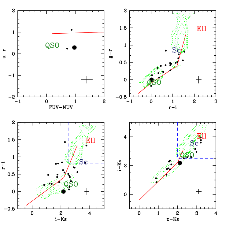
Figure 2: Colour-colour diagrams used as diagnostic of the nature of the observed sources. Dots mark the sources in the present study. Note that the number of points necessarily changes from panel to panel, according to source detection rates in each band. The large dot refers to S0927. Comparison sources are quasar (QSO), elliptical (Ell) and spiral (Sc) galaxy templates redshifted to $z=0.7$ and the loci of main sequence stars according to Girardi et al. (2005) (solid line). The dotted contours refer to the distribution of spectroscopically confirmed stars in the SDSS+2MASS, in a $5\times 5$ square degrees area around S0927 (note that the SDSS spectroscopic survey is inefficient at detecting main sequence stars, hence this comparison is merely qualitative of the scatter around Girardi’s model). The colour cuts described in the text are shown with dashed boxes. Typical error bars on the colours are also indicated in the bottom-right corner of each panel.

The (FUV-NUV,$u$-$r$) plane allows us to infer the nature of the bluest sources. Due to the shallowness of the All Sky Survey, only 3 sources are detected by GALEX: n.15, n.16 and n.40. The first two are S0927 and a companion source $\sim 0.5$ mag fainter in all the observed bands. We suggest that this is a quasar with a redshift close to $0.7$. Source n.40 is a clearly resolved low-redshift irregular galaxy, the stellar population of which is dominated by young stars, as confirmed by our plot.

The ($g$-$r$,$r$-$i$) diagram shows that the sources detected in all these bands are consistent with Galactic stars following the Main Sequence. Only the reddest sources ($g$-$r>1.2$ and $r$-$i>0.8$) are marginally consistent with the Sc template at $z=0.7$ (e.g. Csabai et al., 2003).

The contribution of NIR data is evident in the ($i$-K_s,$r$-$i$) and ($z$-K_s,$i$-K_s) diagrams, where many more red sources are detected. Again, only the reddest sources ($i$-K_s$>2.5$ and $z$-K_s$>2$) are consistent with galaxies at $z=0.7$. Colour cuts are a simplified adaption of those adopted in Blanc et al. (2008) (where we adopt $i^{\rm AB}\approx i^{\rm SDSS}$, $z^{\rm AB}\approx z^{\rm SDSS}$ K${}_{s}^{\rm AB}$=K${}_{s}^{\rm MDM}$+$1.9$).

All the adopted colour cuts favour false-positive detections, and heavy contamination from very red stars is expected. As a consequence, the number of $z\approx 0.7$ galaxy candidates found has to be considered an upper limit.

In Table LABEL:tab_classif, we list the 32 sources for which at least two colours are available. In addition to the quasar hosts n.15 (S0927) and n.16, four sources (n.1, 2, 10, 27) satisfy all the colour selections we set for $z\approx 0.7$ galaxies, in the bands they are detected. A further three sources (n.34, n.56 and n.62) fulfill all but one constraint. Finally, n.32 and n.33 are consistent with 2 out of 4 colour conditions. The number of galaxy candidates at $z\approx 0.7$ is thus 6 (4 quiescent galaxies + 2 quasar hosts), with at most 5 extra ‘lower quality’ candidates. On the other hand, our colour-colour diagrams show that 21 out of 77 sources have colours inconsistent with galaxies at $z=0.7$. We argue that they are Galactic stars or lower redshift galaxies.

Heckman et al. (2009) find 10 galaxy candidates South-West of S0927. Indeed, 6 out of 11 candidates from our analysis are found in the South-West quadrant. Though, since Heckman et al. (2009) do not provide any other indication on the position of their candidates, we cannot assess whether they match ours or not.

6 Comparison with expectations

In order to evaluate whether the number of sources we find is consistent with the galaxy cluster scenario, we must take into account the expected number of contaminating detections in the field of S0927, i.e. field galaxies, stars and quasars. Then we will compare the remaining source counts with the expectations for a typical galaxy cluster at $z\approx 0.7$, given our flux limit. We will focus on the detections from the K_s image, which is much deeper than other available data and probes the rest-frame J-band of galaxies, i.e. is almost insensitive to the age of the stellar populations. Furthermore, given the shallowness of the SDSS images and the red colours of galaxies at $z=0.7$, only the brightest galaxies in the observed K_s-band luminosity function (K${}_{s}\mathrel{\hbox to0.0pt{\lower 3.0pt\hbox{$\sim$}\hss}\raise 2.0pt\hbox{$<$}}17$, see the colour cuts in Figure 2 and the limiting magnitudes in Table 1) can also be detected in the available optical images.

6.1 Field galaxy, star and quasar surface densities

i- Galaxies:

We first compare with the average surface density of galaxies and stars from the general field, following the approach presented in Fukugita et al. (2004). From the MUSYC survey, Blanc et al. (2008) evaluate the galaxy number counts per square degrees in the K_s-band. Considering all the sources flagged as ‘pBzK’ or ‘sBzK’ in the MUSYC survey, that is all bona fide galaxies, and dropping all the objects fainter than our K_s-band sensitivity limit, the expected surface density is $\approx 2.7$ galaxies per square arcmin, that is, $\sim 25$ galaxies in our field. The galaxy surface density estimate provided by Blanc et al. (2008) has a 10 per cent uncertainty, accounting for cosmic variance and Poissonian errors.

ii- Stars:

Through the TRILEGAL software, we also estimate the expected number of Galactic stars in the direction of S0927. Assuming a Chabrier log-normal initial mass function and a thin-disc model of the Galaxy with 2.8 kpc of scale radius (see Girardi et al., 2005, for details), we estimate that the expected number of stars with K_s$<19.45$ in our frame is $\sim 11$. Adopting different assumptions in terms of stellar initial mass function and Galactic disc scale radius yields expected counts ranging from $\sim 5$ to $\sim 18$.

iii- Quasars:

The number of expected quasars per square degree is negligible in this comparison: If we extrapolate the results by Croom et al. (2004), and assume an order-of-magnitude colour transformation B-K_s$\sim$4 for $z\mathrel{\hbox to0.0pt{\lower 3.0pt\hbox{$\sim$}\hss}\raise 2.0pt\hbox{$<$}}2.5$ objects (see, for instance, Hewett et al., 2006), we expect $\sim 0.3$ quasars in our field, that is, $100\times$ smaller than the number of galaxies. Relaxing the B-K_s assumption to $3<$ B-K_s $<5$, the expected quasar counts in our frame would range between $\sim 0.2$ and $\sim 0.5$.

We thus conclude that, on the basis of simple statistics, $\sim 25$ out of the 47 sources detected in our K_s image are possibly field galaxies at any redshift, while 11 are expected to be Galactic stars. The remaining 11 sources can be accounted for in terms of cosmic variance or relaxing some of the assumptions we make in the estimates of field source counts. As a simple estimate, assuming a Poissonian distribution for the expected number of observable field sources (stars+galaxies), we expect $\pm$12 sources within a 2-$\sigma$ deviation. Given those uncertainties our estimate of the field sources is consistent with the number of sources detected in our K_s image. Nevertheless, hereafter we will consider the eventuality that they represent the tip of the iceberg of a galaxy over-density associated to the S0927 system.

6.2 Expectations for a galaxy cluster at $z\approx 0.7$

Here we evaluate whether the observed counts are consistent with the expectations for a cluster at $z\approx 0.7$. The knee of the K_s-band luminosity function of galaxies at this redshift (e.g. Cirasuolo et al., 2008) corresponds to an apparent magnitude $m_{\rm Ks}\sim 18.5$, that is, one magnitude brighter than our detection limit. Firstly we will compare our results to two galaxy clusters in the nearby Universe studied in great detail. Then, we will step to high redshift and consider what is actually observed in known $z\sim 0.7$ clusters.

We use the Virgo and Coma clusters as low-$z$ comparison terms. We emphasize that the velocity dispersion of galaxies in Virgo is only $\sim 600$ km s^-1 (as derived from the GOLDMine Database, see Gavazzi et al., 2003), while it is $1080$ km s^-1 in Coma (Colless & Dunn, 1996). In comparison the measured velocity of S0927 ($\approx 2600$ km s^-1) implies a considerably larger cluster mass, in the assumption that the the shift in the emission lines reflects the cluster velocity dispersion. Nevertheless, Virgo and Coma provide conservative lower limits to the number of galaxies that should be observed in the S0927 field. Moreover, it will also allow us to take advantage of the wealth of information available for low-$z$ galaxies. In particular, we will refer to the GOLDMine Database (Gavazzi et al., 2003) for multi-band photometry, to Gavazzi et al. (1999) for the 3D structure of the Virgo Cluster, and to Eisenhardt et al. (2007) for Coma.

In order to shift Virgo and Coma to $z=0.7$, the following corrections are applied:

Distances and angular scales

– The Distance Moduli of Virgo and Coma are $31.2$ and $35.1$ mag, assuming luminosity distances of 17 and 96 Mpc respectively (Gavazzi et al., 1999, 2003). Therefore, each galaxy moved to $z=0.7$ should appear $12.0$ and $8.1$ mag fainter (without considering any colour and filter correction: see below). The $3.6\times 2.6$ square arcmin field of our study corresponds to $\sim 5.2\times 3.8$ square degrees at the actual distance of the Virgo Cluster, and to $\sim 55\times 40$ square arcmin for Coma. We dropped from our analysis all the galaxies lying outside of boxes with these widths centered on M87 and NGC 4889, where the galaxy density is the highest.

Colour and filter corrections

– In order to minimize the effects of filter and $k$-corrections, we convert the rest-frame J magnitudes into observed K_s magnitudes assuming the galaxy E–Sc templates presented in Mannucci et al. (2001). The coverage of GOLDMine and of Eisenhardt et al. (2007) photometry is practically complete in the bright side of the luminosity function (Gavazzi et al., 2000).

Rejuvenation of stellar populations

– The stellar population of galaxies grew old in the 6.3 Gyr from $z=0.7$ to $z=0$. A detailed correction for this effect is challenging, since the star formation history of galaxies is mostly unknown. For the sake of simplicity, we adopt the parameterization proposed by Gavazzi et al. (2002), with the scale age of the star formation history changing according to the galaxy type and magnitude, following Cortese et al. (2008). On the other hand, NIR emission is insensitive to young stellar populations, and fades out relatively slowly. All the rejuvenation tracks of interest imply corrections ranging between $0.5$ and $1.1$ magnitudes.

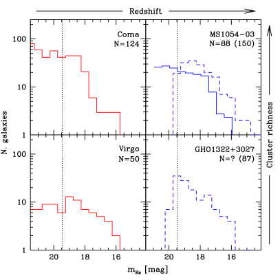
Figure 3: The expected K_s-band galaxy counts of the Virgo, Coma, GHO 1322+3027 and MS 1054-03 Clusters, once “moved” to $z=0.7$ as described in the text. We note that we sampled different regimes of cluster richness both at low and high-redshift. The flux limit of our data is marked with a vertical dotted line. Solid lines refer only to those galaxies belonging to the clusters, while dashed lines are not corrected for the contaminations of foreground sources. The number of objects exceeding our sensitivity limits are also given in the case the correction for foreground sources is (is not) applied.

The resulting luminosity functions are plotted in Figure 3, left. We adopt the same flux cut as in our data, assuming that all galaxies are practically point-like sources at $z=0.7$. We find that 50 sources are expected to be detected in our K_s image, assuming that we are pointing at the core of a Virgo cluster twin centered on S0927, and 124 in the case of Coma. Such high numbers of galaxies are in sharp constrast with respect to the 11 ‘extra’ sources we observe, after star and field galaxy subtraction (see §6.1).

We cannot extend this comparison to other bands because of the poor statistics resulting from the relative shallowness of SDSS photometry. For instance, we can derive the $z$-band expected luminosity function from GOLDMine V-band imaging of Virgo galaxies, and applying the same analysis described above. Nevertheless, once the $m_{z}<20.07$ flux limit is applied, only 8 sources are left. Such small numbers make this comparison inconclusive.

We now consider, as an additional check, the properties of observed galaxy clusters at $z\approx 0.7$. We will focus on the photometric catalogue by Stanford et al. (2002). Among the $z\sim 0.7$ clusters in their analysis, we select GHO 1322+3027 ($z=0.755$, $L_{\rm X}=0.14\times 10^{45}$ erg/s) and MS 1054-03 ($z=0.8231$, $L_{\rm X}=3.37\times 10^{45}$ erg/s) in order to probe two different regimes of cluster richness, as suggested by their X-ray luminosities. In particular, Tran et al. (1999) reported that the stellar velocity dispersion for MS1054-03 is $\sim 1200$ km/s, i.e. roughly half of the velocity difference observed between the red-NEL and the blue line systems in S0927.

In Figure 3, right, we plot the number of objects observed in GHO 1322+3027 and MS 1054-03 as a function of their K_s-band magnitude. In order to allow a direct comparison with our results, we again shift the distributions of $0.2$ and $0.4$ mag respectively, to take into account the different distance moduli with respect to S0927. Filter corrections from the observations of Stanford et al. (2002) and ours and stellar population aging effects are negligible. Up to 87 and 150 sources exceeding our sensitivity limit are expected in these fields, that is, a factor 2 or 3 more than the total observed sources in our K_s-band image of the S0927 field. Concerning MS 1054-03, Förster Schreiber et al. (2006) isolated the contribution of galaxies residing in the redshift range of the cluster (thus excluding most contaminating foreground and background objects). From their analysis, we infer that if S0927 were hosted in a cluster of galaxies similar to MS 1054-03, $\sim 90$ galaxies with $z\approx 0.7$ and $m_{\rm Ks}<19.45$ would be expected: again, many more than the observed.

We remark that, if we consider a lower threshold in the source detection, e.g., we consider all objects with fluxes larger than 2 times the sky count RMS in the PSF area, the “extra” sources would be 17 instead of 11. Such a number is still 3 times below the predictions for a cluster such as Virgo, and 5 (7) times fewer than those expected for a cluster similar to MS 1054-03 (Coma).

7 Discussion and conclusions

In this paper we present a deep K_s-band image of the $3.6\times 2.6$ square arcmin field around S0927. We report the detection of 47 additional sources with $m_{\rm K_{s}}<19.45$. These sources slightly exceed the expectations from general field galaxy and star counts, but are much too few to be consistent with the presence of a galaxy cluster in the field of view.

We match the NIR information with archive GALEX FUV-NUV and SDSS $ugriz$ photometry, and we confirm that 6-11 sources are consistent with galaxies at $z\approx 0.7$. Nevertheless, available optical imaging is so shallow that our colour-based criteria can be applied only to 32/77 (42 per cent) of the sample.

Using Virgo, Coma and the high-$z$ clusters GHO 1322+3027 and MS1054-03 for comparison, we find that the sources observed in our K_s image are several times fewer than expected if a similar cluster surrounded S0927. The velocity dispersions of galaxies in Virgo, Coma and MS 1054-03 are $\sim 600$, $1080$ and $\sim 1200$ km/s, while the redshift differences of the line systems of S0927 correspond to $2650$ km/s, that is, at least a 2-$\sigma$ deviation. If the alleged cluster surrounding S0927 would be richer (so that its velocity dispersion would be higher), the expected galaxy counts will be even higher, which increases the disagreement with the present analysis.

Summarizing, our analysis strongly disfavours the galaxy cluster interpretation of S0927. As already suggested in Heckman et al. (2009), future deep X-ray imaging of the field will provide an alternative independent check for the presence of a massive galaxy cluster in the S0927 field. This may be especially important to probe clusters with extremely low luminous to dark (dark matter + hot gas + diffuse light) mass ratios.

Table 2: List of the sources detected in at least one band in this analysis. (1) source ID; (2–3) RA and dec (J2000); (4–5) GALEX FUV and NUV magnitudes; (6–10) SDSS $ugriz$ magnitudes; (11) K_s-band magnitudes.

ID	RA(J2000)	Dec(J2000)	FUV	NUV	$u$	$g$	$r$	$i$	$z$	Ks
			[mag]	[mag]	[mag]	[mag]	[mag]	[mag]	[mag]	[mag]
1	$09:27:11.9$	$+29:43:12$					$21.77$	$20.44$	$19.89$	$16.67$
2	$09:27:11.5$	$+29:43:27$						$21.07$	$20.33$	$17.12$
4	$09:27:10.9$	$+29:42:58$						$21.20$		$17.75$
5	$09:27:11.9$	$+29:43:30$								$19.48$
7	$09:27:12.8$	$+29:43:40$								$19.17$
8	$09:27:10.5$	$+29:43:34$					$21.36$	$21.06$		$18.36$
10	$09:27:10.2$	$+29:42:56$					$21.90$	$21.07$		$17.39$
11	$09:27:10.3$	$+29:43:14$								$18.42$
12	$09:27:10.2$	$+29:43:24$						$21.36$		$17.73$
13	$09:27:09.6$	$+29:43:03$						$21.48$		$17.81$
15	$09:27:12.6$	$+29:43:44$	$19.45$	$18.48$	$18.69$	$18.42$	$18.40$	$18.40$	$18.34$	$16.22$
16	$09:27:13.8$	$+29:43:35$	$19.94$	$19.22$	$19.38$	$19.18$	$19.14$	$19.01$	$19.13$	$16.42$
17	$09:27:07.9$	$+29:43:00$								$19.23$
18	$09:27:09.0$	$+29:43:33$						$21.56$		$19.45$
19	$09:27:12.9$	$+29:42:34$				$21.90$	$21.01$	$20.59$		$17.97$
20	$09:27:13.3$	$+29:42:27$				$22.22$		$20.83$		$18.14$
24	$09:27:14.8$	$+29:43:21$				$20.28$	$19.35$	$18.89$	$18.82$	$16.31$
26	$09:27:09.8$	$+29:43:34$						$21.15$		$17.29$
27	$09:27:10.2$	$+29:43:43$						$20.79$	$20.40$	$17.19$
28	$09:27:08.0$	$+29:43:28$								$18.11$
29	$09:27:09.7$	$+29:43:43$								$19.40$
31	$09:27:12.3$	$+29:44:13$			$21.12$	$20.92$	$20.92$	$21.10$
32	$09:27:09.2$	$+29:42:21$				$21.18$	$19.92$	$19.30$	$19.24$	$17.15$
33	$09:27:09.7$	$+29:44:21$				$21.67$	$20.13$	$19.32$	$19.03$	$17.51$
34	$09:27:16.6$	$+29:43:07$				$21.12$	$19.65$	$19.09$	$18.86$	$15.94$
35	$09:27:16.8$	$+29:43:09$				$21.89$	$21.21$	$20.37$	$19.97$	$18.29$
36	$09:27:16.3$	$+29:43:12$						$21.37$
39	$09:27:07.3$	$+29:44:03$				$21.17$	$20.50$	$20.08$	$19.95$	$18.34$
40	$09:27:12.8$	$+29:42:11$	$20.33$	$19.46$	$19.73$	$18.96$	$18.62$	$18.43$	$18.49$	$17.59$
46	$09:27:16.9$	$+29:42:27$				$21.85$	$21.48$	$21.42$		$18.85$
47	$09:27:17.1$	$+29:42:30$								$19.03$
48	$09:27:16.5$	$+29:42:48$					$21.82$	$21.02$		$19.37$
49	$09:27:16.9$	$+29:42:44$					$21.57$	$21.02$		$18.77$
51	$09:27:16.0$	$+29:43:45$				$21.95$	$21.06$	$20.79$		$18.91$
52	$09:27:16.1$	$+29:44:08$				$21.58$	$21.03$	$20.80$		$19.59$
53	$09:27:06.0$	$+29:43:31$						$21.43$		$18.28$
55	$09:27:12.4$	$+29:42:17$								$17.67$
56	$09:27:14.0$	$+29:44:20$					$21.13$	$20.44$	$20.48$	$17.49$
57	$09:27:15.0$	$+29:44:03$					$21.63$	$20.93$		$18.04$
58	$09:27:14.3$	$+29:44:05$								$19.05$
61	$09:27:17.5$	$+29:43:43$			$17.64$	$16.15$	$15.58$	$15.36$	$15.43$	$14.00$
62	$09:27:04.8$	$+29:43:07$				$21.00$	$19.78$	$19.27$	$19.09$	$16.76$
63	$09:27:04.5$	$+29:44:01$				$20.69$	$19.81$	$19.33$	$19.09$	$18.21$
64	$09:27:18.1$	$+29:42:35$				$21.96$	$20.68$	$19.95$	$19.67$
65	$09:27:18.5$	$+29:43:18$					$20.90$	$19.47$	$18.75$	$17.19$
66	$09:27:17.4$	$+29:44:09$						$20.44$	$19.70$	$18.09$
67	$09:27:18.8$	$+29:42:55$				$21.44$	$21.15$	$20.81$
68	$09:27:05.5$	$+29:43:28$				$22.23$	$21.09$	$20.60$	$20.29$	$18.84$
70	$09:27:04.4$	$+29:42:42$						$21.00$		$19.08$
73	$09:27:18.2$	$+29:43:07$						$21.49$		$18.28$
74	$09:27:18.4$	$+29:43:09$						$21.34$
75	$09:27:05.1$	$+29:43:08$				$21.29$	$20.84$	$20.44$	$20.16$
76	$09:27:12.8$	$+29:43:48$						$21.26$		$17.47$
77	$09:27:13.8$	$+29:43:33$								$17.80$

Table 3: Classification of the sources according to our colour-colour diagrams. (1) source ID; (2–5) source colours; (6–9) is the colour constraint satisfied? (see text for details) (10) source classification.

ID	$g$-$r$	$r$-$i$	$i$-Ks	$z$-Ks	$g$-$r$	$r$-$i$	$i$-Ks	$z$-Ks	Source
	[mag]	[mag]	[mag]	[mag]	$>1.2$?	$>0.8$?	$>2.5$?	$>2.0$?	classification
1		$1.33$	$3.77$	$3.22$		Y	Y	Y	$z\approx 0.7$ Gal
2			$3.95$	$3.21$			Y	Y	$z\approx 0.7$ Gal
8		$0.30$	$2.70$			N	Y		Star?
10		$0.83$	$3.68$			Y	Y		$z\approx 0.7$ Gal
15	$0.02$	$0.00$	$2.18$	$2.12$	N	N	N	Y	$z\approx 0.7$ QSO
16	$0.04$	$0.13$	$2.59$	$2.71$	N	N	Y	Y	$z\approx 0.7$ QSO
19	$0.89$	$0.42$	$2.62$		N	N	Y		Star?
24	$0.93$	$0.46$	$2.58$	$2.51$	N	N	Y	Y	low-$z$ Gal
27			$3.60$	$3.21$			Y	Y	$z\approx 0.7$ Gal
31	$0.00$	$-0.18$			N	N			Star
32	$1.26$	$0.62$	$2.15$	$2.09$	Y	N	N	Y	$z\approx 0.7$ Gal?
33	$1.54$	$0.81$	$1.81$	$1.52$	Y	Y	N	N	$z\approx 0.7$ Gal?
34	$1.47$	$0.56$	$3.15$	$2.92$	Y	N	Y	Y	$z\approx 0.7$ Gal?
35	$0.68$	$0.84$	$2.08$	$1.68$	N	Y	N	N	Star
39	$0.67$	$0.42$	$1.74$	$1.61$	N	N	N	N	Star
40	$0.34$	$0.19$	$0.84$	$0.90$	N	N	N	N	low-$z$ Gal
46	$0.37$	$0.06$	$2.57$		N	N	Y		Star
48		$0.80$	$1.65$			N	N		Star
49		$0.55$	$2.25$			N	N		Star
51	$0.89$	$0.27$	$1.88$		N	N	N		Star
52	$0.55$	$0.23$	$1.21$		N	N	N		Star
56		$0.69$	$2.95$	$2.99$		N	Y	Y	$z\approx 0.7$ Gal?
57		$0.70$	$2.89$			N	Y		Star?
61	$0.57$	$0.22$	$1.36$	$1.43$	N	N	N	N	Star
62	$1.22$	$0.51$	$2.51$	$2.33$	Y	N	Y	Y	$z\approx 0.7$ Gal?
63	$0.88$	$0.48$	$1.12$	$0.88$	N	N	N	N	Star
64	$1.28$	$0.73$			Y	N			Star?
65		$1.43$	$2.28$	$1.56$		Y	N	N	Star?
66			$2.35$	$1.61$			N	N	Star
67	$0.29$	$0.34$			N	N			Star
68	$1.14$	$0.49$	$1.76$	$1.45$	N	N	N	N	Star
75	$0.45$	$0.40$			N	N			Star

References

- Adelman-McCarthy et al. (2008) Adelman-McCarthy J.K., Agüeros M.A., Allam S.S., Allende P.C., Anderson K.S.J., Anderson S.F., Annis J., Bahcall N.A. et al., 2008, ApJS, 175, 297
- Bahcall (1978) Bahcall N.A., 1975, ApJ, 198, 249
- Bessell & Brett (1988) Bessell M.S. & Brett J.M., 1988, PASP, 100, 1134
- Blanc et al. (2008) Blanc G.A., Lira P., Barrientos L.F., Aguirre P., Francke H., Taylor E.N., Quadri R., Marchesini D. et al., 2008, ApJ, 681, 1099