CPT-P036-2009

ITFA-12-2009

Spatial ’t Hooft loop in hot SUSY theories at weak coupling

Chris P. Korthals Altes

Centre Physique Théorique au CNRS

Case 907, Campus de Luminy

F-13288 Marseille, France, and

Institute Theoretical Physics

Valkeniersstraat 65

1018 XE, Amsterdam, the Netherlands

altes@cpt.univ-mrs.fr

Abstract

The spatial ’t Hooft loop measures the colour electric flux in SU(N)/Z(N) gauge theory. It is a closed loop of Dirac Z(N) flux and has strength k=1, 2,.., N-1. It is analyzed for generic k and small gauge coupling in the high temperature phase of N =1, 2 and 4 SUSY theory up and including cubic order. In one loop order no qualitative difference with gluodynamics shows. However the two loop order shows a logarithmic divergence appear in the centre of the wall. This is because the gluinos become bosonic in the centre and acquire long wavelength excitations. We discuss the cure for this divergence, due to a gluino zero mode. The physics of Casimir scaling is explained. The cubic order can be obtained from gluodynamics by simple rescalings of the Debye masses and the Casimir parameter $k/N_{c}$.

1 Introduction

The physics at RHIC is that of a strongly interacting plasma. In this regime QCD can only be studied on the lattice like the smallness of the shear viscosity over entropy ratio (for a review see ref. [1]). Many questions are still beyond the reach of simulations, like the fast rate in going to equilibrium. This is one of the reasons to contemplate the AdS/CFT connection and its non-equilibrium ramifications [6]. The CFT is four dimensional high temperature ${\cal N}=4$ SUSY, and can be studied in strong coupling by the calculating in the five dimensional bulk theory in weak coupling. Another reason lies in the Z(N) reduced effective actions [14] and their plethora of undetermined parameters in the the case of gluodynamics: maybe their SUSY counterparts have more to say about his.

The thermodynamics of N=4 SUSY has been analysed about ten years ago [10][11][12]. These authors obtained weak coupling results for the free energy and the Debye mass, in order to see how they connected to strong coupling results from the AdS/CFT approach.

Recently other observables have been studied, like the mean colour-electric flux in the plasma measured by the spatial ’t Hooft loop [16].

Their results for small coupling are one-loop precision. To this order nothing qualitative distinguishes the ${\cal N}=4$ case from gluodynamics. In this note we will compute the loop to the next order. This involves two-loop calculations which are remarkably simple in gluodynamics [8] and stay so in SUSY. However the results become in this order qualitatively different from gluodynamics.To two loop precision this effect is signaled by a divergence in the tension. How to cure this divergence is discussed in section  6. This divergence is due to a gluino zero mode [15].

When doing the calculation it is expedient to use the multidimensional formulation for SUSY theories [5]. Not only ${\cal N}=4$, but also ${\cal N}=2,1$ cases are covered to the order we compute by a single parameter $\delta$, the dimension used.

Our results may then be contrasted with those of strong coupling in ref. [16] in ${\cal N}=4$.

In section 2 the problem is set up and the results for the effective potential are stated. In section 3 some technicalities of our perturbative method to obtain the effective action are given, in the next section  4 the physical reason for Casimir scaling is belaboured. Both of the latter sections can be skipped by the reader who is imainly interested in the results. The minimization of the effective potential to obtain the tension associated to the ’t Hooft loop is done in section 5. The results are discussed in the next section and we wind up with conclusions. Some appendices are included to support claims in the main text.

2 The set-up and the results

Consider the plasma of a four dimensional SU(N) gauge theory with only adjoint coloured matter, like gluodynamics or N=1,2 or 4 SUSY. Such a theory admits SU(N) gauge transformations with a discontinuity in the center Z(N) of SU(N). In particular one can imagine a closed macroscopic spatial loop L of Dirac magnetic flux [2]. Such a loop is given by any static gauge transformation $V_{k}(L)$ that picks up a discontinuity $z_{k}=\exp(ik{2\pi\over N})$, whenever we circumnavigate the loop, say clockwise. In fig.2(a) we show such a situation, with the loop in the (y,z) plane.

The claim is that the quantum average of such a loop measures the mean colour electric flux through the loop. The quantum average is of course the Boltzmann trace, up to a normalizing factor:

$$\langle V_{k}(L)\rangle=\mbox{Tr}~{}V_{k}(L)\exp(-H/T).$$ (1)

The trace is over all the colourless, i.e. gauge invariant states in our theory. This is the quantity we will compute to two loop order for SUSY theories. Like its homologue in gluodynamics [8] it has a rapid exponential fall-off, in fact with the area $A(L)$ of the loop:

$$\langle V_{k}(L)\rangle=\exp(-\varrho_{k}A(L)).$$ (2)

The quantity $\varrho_{k}$ that controls this fall-off is called with a remarkable misnomer the ”tension”, or ”dual string tension”.

Before we delve into formalism a few words on what we can expect on the basis of simple arguments. The spatial t Hooft loop is the SU(N) version of the Dirac string in quantum-electrodynamics.

The Dirac string is engineered such that it is undetectable by quantum particles: the wavefunction of any particle in the theory, boson or fermion, is unaffected by the presence of the loop. The strength of the string is then equal to the total magnetic flux coming out of the monopole at its end. If it has two endpoints it describes a monopole-antimonopole pair. The strength of the string is the number of times the phase of the gauge transformation winds around the gauge group U(1). For the ’t Hooft loop the gauge group is $SU(N)/Z(N)$

The spatial ’t Hooft loop $V(L)$ is a macroscopic Dirac string $L$ closed on itself. From its unobservability it would naively seem to be an academic object. However this needs not to be true at low temperatures, where the macroscopic quantum-mechanical coherence of a condensate can create Abrikosov flux tubes. Under such circumstances  the spatial loop, or rather the state created by it from the ground state, will acquire an energy proportional to its perimeter.

There is a less well known role played by the spatial ’t Hooft loop. Mathematically, our closed Dirac string can rewritten through the use of Gauss’ law as generator of gauge transformations as an electric flux loop [3] (see also next subsection):

$$V(L)=\exp(i4\pi{\int_{S(L)}d\vec{S}.\mbox{Tr}\vec{E}Y_{k}/g}).$$ (3)

$Y_{k}$ is a suitably chosen colour matrix in the fundamental representation , the hypercharge generating the Z(N) transformation ($\exp(i2\pi Y_{k})=\exp(ik(2\pi/N)){\bf 1})$, and g is the gauge coupling. $\vec{E}$ is the electric field strength in the fundamental representation. Since gluons are in the adjoint representation of $SU(N)/Z(N)$ their hypercharge is $\pm 1$ or $0$, whatever the value of k. What does depend on k are the multiplicities.

Once more one would say off-hand that no quantum particle in the theory will detect the area. However one might argue that at very high temperatures the thermally screened particles are getting close to behaving as classical particles, escaping therefore the Dirac veto. This statement is correct in the limit of small coupling, where the classical Debye screening length $\lambda_{D}\sim{1\over{gT}}$ is very large compared to the de Broglie wave length $\lambda_{B}\sim{1\over T}$.

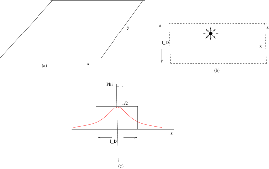
Figure 1: Flux loop (a), Debye slab of thickness $\lambda_{D}$ with particle emitting its flux (b), behaviour of flux as function of distance from the loop (red) in (c), and simplified (black)

In that situation one can consider the slab (see fig. (1 (b)) to be a thin slab of width $\lambda_{D}$, where independent particles contribute to the flux through the loop. This is shown in fig. (1(c).) It is then not hard to see [18] that one particle will contribute -1 to the flux (because only half of its flux shines through the loop, giving $\exp(i\pi)$), two independent particles $(-1)^{2}$, etc..

The Poisson distribution for a given species of screened gluons is that of Boltzmann particles in the fiducial volume -with on average $\bar{l}=n\lambda_{D}\mbox{A(L)}$, n the density of the species-. It reads:

$$P(l)={{\bar{l}}^{l}\over{l!}}\exp(-\bar{l})$$ (4)

and so the flux average for this single species is:

$$\sum_{l=0}^{\infty}P(l)(-)^{l}=\exp(-\lambda_{D}n(T)\mbox{A(L)}).$$ (5)

Taking all species of gluons into account one has to determine how many gluons in the adjoint are having a non-zero charge $AdY_{k}$ . This turns out to be $2k(N-k)$. Because of the independence of the particles the exponent for one species is multiplied by this multiplicity:

$$\varrho_{k}\mbox{A(L)}=2k(N-k)\lambda_{D}n(T)\mbox{A(L)}.$$ (6)

$\varrho_{k}$ is the quantity controlling the area-off defined in eq. (2), called the tension. It has nothing to do with a tension. The density $n$ is the same everywhere inside and outside the minimal area of the loop. It just tells us how the fall-off of the mean flux is controlled by the type of particles we have in the theory. The Casimir scaling is a signature for the adjoint representation. Evidently, in the confined phase we have no area law anymore as the colour electric flux is enclosed inside the hadrons.

Coming back to gluodynamics, in leading order in perturbation theory this result (6) was qualitatively reproduced [8], with the Casimir scaling factor $k(N-k)$ and the factor $\lambda_{D}\sim 1/g$. And indeed on the lattice [17] Casimir scaling is valid, not only at very high T, but surprisingly almost down to the critical temperature! Of course the simple coupling constant behaviour in our leading order result (6) is only valid at very high temperature. Lowering T will increase the coupling. For gluodynamics the two loop results are known [8][18], and so are the cubic terms [19]. The cubic results are numerically small, but do violate Casimir scaling. Everything we know is consistent with the hypothesis that hard physics (on the scale T) respects Casimir scaling and that soft physics (on the scale gT) does not.

For SUSY theories the gluons are accompanied by scalars and gluinos, all of them in the adjoint of SU(N). So we expect Casimir scaling according to the arguments above.

In this paper we will push the perturbation series to two loop order and will argue that the next, cubic, order is just a suitable rescaling of results known from gluodynamics.

In next to leading order we will find again Casimir scaling. This is not surprising as we argue in section 4. But to three loop order one needs a dynamical mechanism to explain cancellations in the planar diagram sector.

First we want to understand how the electric flux formula (3) comes about.

2.1 What has the spatial loop to do with mean colour electric flux?

First let us produce an explicit version of such a singular gauge transform.

A set of Lie-algebra matrices $Y_{k}$ that generates the center through $z_{k}{\bf 1}=\exp(i2\pi Y_{k})$ is [18]:

$$Y_{k}={1\over N}~{}{\rm diag}(\underbrace{k,k,\dots,k}_{N-k~{}{\rm times}},\underbrace{k-N,k-N,\dots,k-N}_{k~{}{\rm times}}).$$

The k are integers.

The Gauss operator is written as:

$$G^{a}=-E_{i}^{b}D^{ab}_{i}.$$ (7)

From the covariant derivative, $\vec{D}=\vec{\partial}+ig[\vec{A},$, we have  :

$$G^{a} = -\vec{E}^{a}.\vec{\nabla}+gf_{abc}A_{i}^{b}E^{c}_{i}$$ (8)

$$gj_{0}^{a} = -gf_{abc}A_{i}^{b}E^{c}_{i}.$$ (9)

The last equation defines the colour charge density $gj_{0}^{a}$.

Our singular gauge transformation is written as

$$\exp(i\omega_{a}\lambda_{a}).$$ (10)

Then we take $\omega_{a}\lambda_{a}\equiv\alpha(\vec{x})Y_{k}$ with $\alpha(\vec{x})$ equal to half the solid angle defined between $\vec{x}$ and L.

The ’t Hooft loop is defined as the operator version of (10):

$$V_{k}(L)=\exp(i\int d\vec{x}G^{a}\omega_{a}).$$ (11)

We integrate inside a large sphere including the loop L the operator density $\vec{\nabla}.(\vec{E}^{a}\omega^{a})$ :

$$\int dV\vec{\nabla}.(Tr\vec{E}\omega)=\mbox{surface term on $S_{\infty}$}-\int_{S(L)}d\vec{S}.Tr\vec{E}Y_{k}2\pi$$ (12)

The surface term is negligeable because of the fall-off of the integrand. In the second term the explicit form of $\omega$ is used.

The l.h.s. is the sum of two terms:

$$\int dV\vec{\nabla}.(Tr\vec{E}\omega) = \int dVTr(\vec{\nabla}.\vec{E})\omega)+\int dV.(Tr(\vec{E}.\vec{\nabla})\omega)$$

$$= \int dVTr(\vec{\nabla}.\vec{E}-gj_{0})\omega+\int dVTr(\vec{E}.\vec{\nabla}+gj_{0})\omega$$

We have added and subtracted the colour charge density to produce Gauss’ operator (9). So the first term cancels on physical states. The second term equals, because of the normalization of the $\lambda$ matrices:

$$\int dVTr(\vec{E}.\vec{\nabla}+gj_{0})\omega={1\over 2}\int dV(\vec{E}^{a}.\vec{\nabla}+gj^{a}_{0})\omega^{a}).$$ (13)

It is the latter integral which is, up to a sign, the gauge transformation (9) and hence, combining eq. (12) and (2.1) and exponentiating we get:

$$\exp({4\pi\over g}i\int_{S(L)}d\vec{S}.Tr\vec{E}Y_{k})=\exp(i{1\over g}\int dV(\vec{E}^{a}.\vec{\nabla}+gj^{a}_{0})\omega^{a})).$$ (14)

in the physical Hilbert space. The r.h.s. is the gauge transformation in Hilbert space of $\exp(i\omega(\vec{x}))$ with a discontinuity $z_{k}$ in the centergroup on the surface. This was the definition of the ’t Hooft loop. On the left hand side we see its representation as an electric flux operator.

Once its role as electric colour flux operator is understood, it is intuitively clear that the average (1) will be an area law in a plasma [18]:

$$\langle V_{k}(L)\rangle=\exp(-\varrho_{k}(T)\mbox{Area(L)}).$$ (15)

The quantity that controls the fall-off is called the electric tension, or ”dual tension”.

Now we return to its quantum average (1) and discuss two other guises for this average.

2.2 Two other guises for the spatial ’t Hooft loop average

The second guise is useful for calculations on the lattice or in perturbation theory and is the Euclidean path integral version. The gauge transformation is replaced by the Polyakov loop in the Euclidean time direction $\tau$:

$$P(A_{0})(\vec{x})={\cal{P}}\big{(}\exp(i\int_{0}^{1/T}d\tau A_{0}(\vec{x},\tau))\big{)}.$$ (16)

Since it transforms under a gauge transformation as an adjoint:

$$P(A_{0}^{\Omega})=\Omega(\vec{x},0)P(A_{0})\Omega^{\dagger}(\vec{x},1/T),$$ (17)

the N-1 phases of the diagonalized loop are invariant under periodic transforms, and shift under periodic modulo centergroup transformation [4].

So the gauge invariant content of the loop can be stored in the trace of N-1 powers of the loop:

$$P^{(k)}(A_{0})=\mbox{Tr}P(A_{0})^{k},~{}~{}\mbox{k=1,......,N-1}.$$ (18)

Imagine the Polyakov loop along a straight line in the x-direction. The straight line pierces the area inside the loop L. in the (y,z) plane. As long as we stay away from the boundary the Polyakov loop will have the same profile on any such line, and will only depend on z. When the Polyakov loop crosses the surface, where the loop operator $V_{k}(L)$ has its discontinuity, it will pick up the discontinuity because of (17).

So what we need is the probability for a given Polyakov loop profile C(z) to appear. C(z) is a diagonal traceless real NxN matrix, obeying

$$P^{(k)}(C)=\mbox{Tr}\exp(ikC/T).$$ (19)

Then we maximize this probability with the boundary conditions at infinity $P(A_{0})(x=\pm\infty)={\bf 1}$ and by the jump at the surface.

The probability is determined by the Euclidean path integral with the constraint:

$${\cal C}=\Pi_{k,x}\delta\big{(}\overline{P^{(k)}(A_{0})}-\mbox{Tr}\exp(ikC/T)\big{)}.$$ (20)

The overlined Polyakov loop is a short hand for the average over y and z coordinates. For this to make sense we put the system in a finite but large transverse volume $V^{tr}$ of the y and z coordinates.

The constraint is inserted in the path integral. We then get, up to the usual partition function for the probability that a given profile in the x direction develops:

$$\int DADSDF~{}~{}{\cal C}\exp(-S)=\exp(-V^{tr}U(C)-\mbox{bulk free energy}).$$ (21)

We integrate over gauge fields A, scalar fields S and fermionic fields F.

$U(C)$ is the resulting effective action. The effective action can be written in terms of a kinetic term $K$ proportional to $\mbox{Tr}(\partial_{z}C)^{2}$ and an effective potential $V(C)$:

$$U(C)=\int dx\Big{(}{1\over{2g^{2}N}}\widehat{K}\mbox{Tr}(\partial_{z}C)^{2}+V(C)\Big{)}.$$ (22)

The (y,z) plane at x=0, where the Polyakov loop jumps, is called a domain wall. This is a little confusing, because we think of a domain wall as a soliton, living sub specie aeternitatis. With only a reinterpretation of the Euclidean coordinate axes we can obtain such a picture, at the price of having either y or z axis as the infinite time axis.

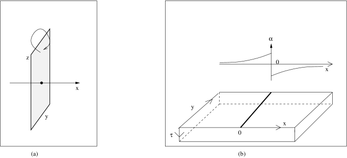
Figure 2: Left panel: the spatial ’t Hooft loop in the (y,z) plane at x=0. The arrow on the upper part indicates the clockwise circumnavigation defining the jump, eq. (11). On the right the same loop but now with the z-axis interpreted as time axis. The (x,y) plane contains a one-dimensional wall at x=0, and a microscopically small, periodic spatial $\tau$-direction along which the Polyakov loop profile $P(C)=\exp(i2\pi T\alpha(x)Y_{k})$ is winding, with the phase $\alpha$ of the profile as function of x shown in panel (b). Fermionic fields are supposed to be anti-periodic in the $\tau$ direction.

Hence the third guise is that of a one dimensional defect, that lives in the two dimensional (x,y) world with a small periodic space dimension labeled $\tau$ (see fig. (2)(b)) . The Euclidean time is now the z-axis, so the temperature is zero. The defect is given by the jump the Polyakov loop looping the small periodic space dimension $\tau$ feels when crossing the line defined by x=0 in the (x,y) plane. Thus the defect is once more a magnetic flux.The energy per unit length of the magnetic flux is again $\varrho_{k}(T)$. It is created at say $z=-L_{z}/2$ and lives on in the z direction during the time $L_{z}$ , that we let go to infinity [25]. Calculationally there is no difference with the second guise, the Euclidean path integral (21).

Its usefulness lies amongst more in an alternative but simpler and elegant understanding of the nature of the divergencies we will meet in the kinetic part of the effective action.

2.3 Results for the effective action for ${\cal N}=1$, 2 and 4 SUSY

For our purpose we follow Vasquez-Mozo [13] and compute with the ${\cal N}=1$ SUSY action formulated in $\delta\geq 4$ dimensions [5]. When $\delta=10$ the fermions are constrained to be Majorana-Weyl fermions, and we recover N=4 SUSY. When $\delta=6$ the fermions are Weyl fermions and we recover ${\cal N}=2$ SUSY. When $\delta=4$ we have by definition ${\cal N}$=1 SUSY, with Majorana fermions. So generically the action we use reads:

$$S=\int d^{4}x\bigg{(}{1\over 2}\mbox{Tr}F_{pq}^{2}+\mbox{Tr}\bar{\lambda}\Gamma_{p}D_{p}\lambda\bigg{)}~{}~{}p,q=0,1,...,\delta-1..$$ (23)

The fields in our action are the bosonic ones $A_{p}$, p=0,1…9, appearing in the field strength $F_{pq}=\partial_{p}A_{q}-\partial_{q}A_{p}+i[A_{p},A_{q}]$. Both fermions and bosons are matrix-valued (in the Lie-algebra of SU(N), and the covariant derivative reads $D_{p}=\partial_{p}+i[A_{p},$.

The fermions $\lambda$ are spinors with $\delta-2$ independent components because of the constraints. Their dimension (and that of the Dirac matrices $\Gamma_{p},p=0,1,...\delta-1$) is $2^{\delta/2}$. All fields only vary with $x_{0}\equiv\tau,x_{1}=x,x_{2}=y,~{}\mbox{and}~{}x_{3}=z$, the remaining dimensions serve as bookkeeping device for the flavours (SU(4) for $\delta=10$, and $U(2)$ for $\delta=6$). In bosonic computations the $\delta$-dimensional unit matrix ${\bf 1}_{b}$ often appears, whereas in their fermionic counterparts the projector matrix ${\bf 1}_{f}\equiv\lambda\times\bar{\lambda}$ ($2^{{\delta\over 2}}$ dimensional) with $\mbox{Tr}{\bf 1}_{f}=\delta-2$ is present. For details see Appendic C.

2.3.1 Some basic facts and notation

We use throughout dimensional regularization with $d=4-2\varepsilon$, $\varepsilon\rightarrow 0$.

The Feynman rules are the Euclidean finite temperature rules, with the Matsubara frequency $l_{0}=2\pi nT$, n integer for bosons, and $l_{0}+\pi T$ for fermions. The constraint (20) will introduce a background $A_{0}=C+gQ_{0}$. Therefore the covariant derivative $D_{0}=\partial_{0}+ig[C,$ will remain in the in the propagators. Hence it is advantageous to go into the Cartan basis for all the quantum fluctuations $gQ_{p}=A_{p}$, for $p\geq 1$ and for the quantum fluctuations $\lambda$. The Cartan basis consists of the off-diagonal matrices $\lambda^{ij}$ with the (ij) entry equal to $1/\sqrt{2}$ and other entries zero. They form an eigenbasis for C:

$$[C,\lambda^{ij}]=(C_{ii}-C_{jj})\lambda^{ij}.$$ (24)

The potential is known, on general grounds [9], to have absolute minima at the locations where $\exp(iC/T)$ takes value in the centergroup.

More specifically [18] the potential valleys of the lowest order (one-loop) potential $V_{1}$ relating the origin to the nearest minimum with Z(N) value $z_{k}$ are described by the matrices (see (2.1):

$$C=2\pi Tq(x)Y_{k}.$$ (25)

The scalar function $q(x)$ is to be determined as function of x from the minimization of U(C). It enters the Matsubara frequencies  as:

$$l_{0}+2\pi Tq~{}~{}\mbox{ for bosons and}$$ (26)

$$l_{0}+\pi T+2\pi Tq~{}~{}\mbox{for fermions.}$$ (27)

Thus, inside the wall the role of bosons and fermions starts to get interchanged. In particular in the center of the wall-where $q=1/2$- the fermions develop long range behaviour in the two dimensions left, just as the bosons do outside the wall at q=0 and 1, but now in three dimensions. We will come back to this phenomenon in section 6.

The summation/integration measure is written as

$$\hbox{$\sum$}\!\!\!\!\!\!\int_{~{}l(b,f)}\equiv T\sum_{n}\int{d^{d-1}l\over{(2\pi)^{d-1}\mu^{2\varepsilon}}},$$ (28)

where the suffix b or f refers to whether we put the bosonic or fermionic Matsubara frequency. The scale $\mu$ starts to play a role in the one loop kinetic term.

We fix the notation for the sum/integrals we meet in the one and two loop. They are proportional to Bernoulli polynomials and read ($l_{q}^{2}\equiv(l_{0}+2\pi Tq)^{2}+\vec{l}^{2}$):

$$\hbox{$\sum$}\!\!\!\!\!\!\int_{~{}l(b)}\log(l_{q}^{2}) = \hat{B}_{4}(q)$$ (29)

$$\hbox{$\sum$}\!\!\!\!\!\!\int_{~{}l(b)}{(l_{0}+2\pi Tq)\over{l_{q}^{2}}} = \hat{B}_{3}(q)$$ (30)

$$\hbox{$\sum$}\!\!\!\!\!\!\int_{~{}l(b)}{1\over{l_{q}^{2}}} = \hat{B}_{2}(q)$$ (31)

$$\hbox{$\sum$}\!\!\!\!\!\!\int_{~{}l(b)}{(l_{0}+2\pi Tq)\over{l_{q}^{4}}} = \hat{B}_{1}(q).$$ (32)

The right hand sides are represented by Bernoulli polynomials $B_{r}$ ( defined in Appendix B) on the interval $-1\leq q\leq 1$. If the trace is fermionic, the argument of the B-polynomials is shifted by ${1\over 2}$. The integrals on the left hand side are periodic mod 1 in the argument q.

Obviously one recovers by differentiation $\hat{B}_{3}$ from $\hat{B}_{4}$, etc., up to some overall factor. As they are periodic ”polynomials” they are not analytic at $q=0,1....$.

Since the breaking of supersymmetry resides in the shift from bosonic to fermionic traces, the non-renormalization of supersymmetric potentials makes differences like

$$D_{r}(q)=\hat{B}_{r}(q)-\hat{B}_{r}(q+{1\over 2})$$ (33)

occur frequently. The number of bosonic (or fermionic) degrees of freedom appears naturally as well. We write

$$\Delta={\delta-2\over 2},$$ (34)

equal to 1, 3 and 4 for respectively ${\cal{N}}=1,2,~{}\mbox{and}~{}4$.

2.3.2 Results for the effective potential

From refs [10][13][12] we quote the one and two loop free energy:

$$F_{1} = \Delta(N^{2}-1)\hat{D}_{4}(0)$$ (35)

$$F_{2} = \left(\Delta\tilde{g}\right)^{2}(N^{2}-1)\hat{D}_{2}(0)^{2},$$ (36)

with $\tilde{g}^{2}$ the ’t Hooft coupling.

The dimension of the adjoint representation appears because each member of a given multiplet has the same weight in the free energy.

The screening masses of the gauge fields are from the same references:

$$m_{D}^{2}={\Delta\over 2}\tilde{g}^{2}T^{2}.$$ (37)

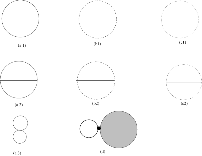
Figure 3: One and two loop contributions to the effective potential. Continuous lines are bosons, broken lines are fermions and dotted lines are ghosts. In (a) the bosonic contributions, in (b) the fermionic contributions and (c) the ghost contribution are shown. In (d) the Polyakov loop (fat circle), renormalized by one gluon exchange, is inserted into the sum of the loops (a1), (b1) and (c), given by the shaded blob.

The potential terms of the effective action read on the interval $0\leq q\leq{1\over 2}$:

$$V = V_{1}+\tilde{g}^{2}V_{2}$$

$$V_{1} = 2k(N-k)\Delta\hat{D}_{4}(q)$$ (38)

$$V_{2} = k(N-k)\Delta\bigg{[}\Delta\bigg{\{}\bigg{(}\hat{D}_{2}(q)+\hat{D}_{2}(0)\bigg{)}^{2}-\hat{D}_{2}(0)^{2}\bigg{\}}+4\hat{B}_{1}(q)\hat{D}_{3}(q)\bigg{]}$$ (39)

The contributions of the individual diagrams are given in Appendix D.

Note the factors $k(N-k)$. They replace the factor $N^{2}-1$ in the free energy and are referred to as ”Casimir scaling”. To one loop order they appear as a consequence of simple counting: for a given charge $Y_{k}$ there are k(N-k) excitations in the adjoint with charge 1 and an equal number with charge -1. As the $\hat{B}_{4}(\pm q)$ take the same value we have Casimir scaling.

For the two loop potential this counting is not enough as there are interactions. In section 4 the double line notation is used to show how Casimir scaling is nethertheless realized.

The factors $\Delta={\delta-2\over 2}$ count the number of $\delta$ dimensional loops. The last term of $V_{2}$ is the exception, for a simple reason. This latter term is due to the one loop renormalization of the Polyakov loop (see fig.(3 (d)), which only involves the gauge sector and is proportional to $B_{1}$:

$$\delta q=-{\tilde{g}^{2}\over{(4\pi)^{2}}}(3-\xi)B_{1}(q)$$ (40)

Inserted into the result for $V_{1}(q)$, $V_{1}(q+\delta q)$, it gives a result linear in ${\delta-2\over 2}$ and $\hat{B}_{3}$. We show in more detail in section 3 how these insertions come about.

To obtain the old result for gluodynamics, put $\delta=4$ and drop the fermionic contributions to find [8]:

$$V_{1}+\tilde{g}^{2}V_{2}=k(N-k){4\pi^{2}\over 3}T^{4}q^{2}(1-q)^{2}\bigg{[}1-5\bigg{(}{\tilde{g}\over{4\pi}}\bigg{)}^{2}\bigg{]}.$$ (41)

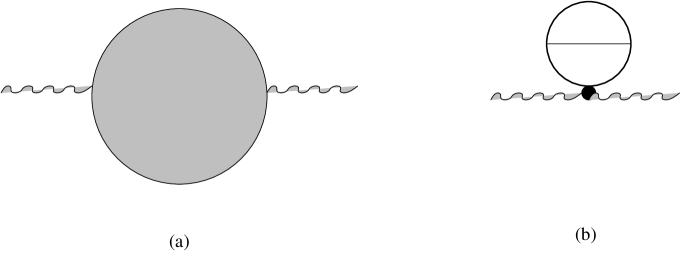
Figure 4: The contributions to the one loop effective kinetic term. The wiggly lines are $q$ lines. The shaded blob in (a) is the sum of one loop boson, fermion and ghost graphs. In panel (b) the renormalization of the Polyakov loop is shown.

2.3.3 One loop kinetic term

We now turn to graph (a) in fig. 4. It is obtained by computing the determinant of boson ghost fields in (68) and expanding the determinant in terms of derivatives of the background. We suppose the colour degrees of freedom have been diagonalized in the Cartan basis $Q^{ij}$, so that the background $B$ below stands for $B^{ij}=B_{ii}-B_{jj}$.

So we have to take into account that the x-dependence in the background does not commute with the momentum operator $P_{x}={1\over i}\partial_{x}$ in the d’Alembertian. The $B$ field will depend on the operator $X$, $\underline{B}\equiv B(X)$, that obeys:

$$[P_{x},X] = -i~{}~{}\mbox{and}$$

$$X|x\rangle = x|x\rangle.$$ (42)

We do this in Feynman gauge $\xi=1$. This gives for the bosonic part of the effective kinetic term ( for the fluctuation matrix see (68):

$$K_{b}=\mbox{Tr}_{b}{1\over 2}\log\bigg{(}-D^{2}(\underline{B}{\bf 1_{b}}-2F_{0x}{\bf 1_{0x}}\bigg{)}-\mbox{Tr}_{b}\log\bigg{(}-D^{2}(\underline{B})\bigg{)}.$$ (43)

The first term is due to vector bosons and scalars, the second logarithm due to the ghost. The magnetic moment term of the gluonic component is proportional to $F_{0x}=B^{\prime}$ and hence ${\cal O}(g)$ and expanded out. The scalar component has no such term, as reflected in the matrix:

$${\bf 1_{0x}}\equiv\mbox{Diag}(1,-1,0,...,0).$$ (44)

So $K_{b}$ becomes:

$$K_{b}={\delta-2\over 2}\mbox{Tr}_{b}\log(-D^{2}(\underline{B}))-{1\over{2!}}F_{0x}^{2}4Tr_{b}{1\over{(-D^{2}(B))^{2}}}\bigg{)}.$$ (45)

We do the same for the fermionic determinant. The result there is different in that the spin terms are present for all fermionic components .

One gets accordingly:

$$K_{f} = -\mbox{Tr}_{f}{1\over 2}\log\bigg{(}-D^{2}(\underline{B}){\bf 1_{f}}-F_{0x}\Gamma_{0x}{\bf 1}_{f})\bigg{)}$$ (46)

$$= -{\delta-2\over 2}\bigg{(}Tr_{f}\log(-D(\underline{B})^{2}-{1\over{2!}}F_{0x}^{2}Tr_{f}{1\over{(-D(B)^{2})}}\bigg{)}.$$

The spin matrix $\Gamma_{0x}={1\over{4i}}[\Gamma_{0},\Gamma_{x}]$.

The trace is mixed in x and conjugate momentum, instead of the pure momentum trace $\hbox{$\sum$}\!\!\!\!\!\!\int$ in section 2:

$$\mbox{Tr}O\equiv=T\sum_{n}\int{d^{d-2}l\over{(2\pi)^{d-2}\mu^{2\varepsilon}}}\int dx\langle x|O|x\rangle.$$ (47)

The suffixes b or f refer to treating the Matsubara frequency $l_{0}=2\pi nT$ as bosonic or fermionic, by adding in the latter case $\pi T$.

The total effective kinetic term is now:

$$K=K_{b}+K_{f}$$ (48)

and from (45) and (46) follows:

$$K = {\delta-2\over 2}\bigg{(}\mbox{Tr}_{b}\log(-D^{2}(\underline{B}))-\mbox{Tr}_{f}\ log(-D^{2}(\underline{B}))\bigg{)}$$ (49)

$$+ {1\over{2!}}F_{0x}^{2}\bigg{(}-4Tr_{b}{1\over({-D^{2}(B))^{2}}}+{\delta-2\over 2}Tr_{f}{1\over{(-D^{2}(B))^{2}}}\bigg{)}$$

The short distance behaviour of the total effective kinetic term is independent of the background and whether the trace is bosonic or fermionic . The short distance contributions of the first two terms in $K_{b}$ and $K_{f}$  do therefore cancel in the effective kinetic term, and we conclude the short distance behaviour of the kinetic part of the SUSY action is fixed entirely by the difference of the magnetic moment terms of bosons ($-4$) and fermions (${\delta-2\over 2}$):

$$K_{shortdistance}\sim{1\over{2!}}F_{0x}^{2}((-4+{\delta-2\over 2})({1\over{\varepsilon}}+{\cal O}(\varepsilon)).$$ (50)

This difference vanishes for $\delta=10$, as it should. If $\delta$ is smaller than 10 we retrieve the asymptotically free SUSY theories. For $\delta$ larger than 10 asymptotic freedom is lost.

Finally, from (116) in Appendix A and (49) the kinetic term equals in $d\rightarrow 4$ and $\delta$ dimensions:

$$K = k(N-k){(2\pi Tq^{\prime}(x))^{2}\over{\tilde{g}^{2}}}\times$$ (51)

$$\times \bigg{[}1+{\tilde{g}^{2}\over{(4\pi)^{2}}}{\Gamma({5-d\over 2})\over{\pi^{{5-d\over 2}}}}\bigg{(}{T\over{\mu}}\bigg{)}^{-2\varepsilon}\bigg{\{}\bigg{(}b_{b}(\delta)+{2\varepsilon\over 3}{\delta-2\over 2}\bigg{)}\sum_{n}{1\over{|n+q|^{5-d}}}$$

$$- \bigg{(}-b_{f}(\delta)+{2\varepsilon\over 3}{\delta-2\over 2}\bigg{)}\sum_{n}{1\over{|n+1/2+q|^{5-d}}}\bigg{\}}-4{\tilde{g}^{2}\over{(4\pi)^{2}}}\bigg{]}$$

The very last ${\cal O}(\tilde{g}^{2})$ term comes from diagram (b) in fig.(4) and results from substituting the renormalization $\delta q=-{\tilde{g}^{2}\over{(4\pi)^{2}}}(3-\xi)B_{1}(q)$ ( see eq. (71)) into the kinetic term $q^{\prime 2}$ in Feynman gauge $\xi=1$ . Details can be found in section 3. The one loop $\beta$-function coefficients $b_{b}$ respectively $b_{f}$ are the contributions of the bosons respectively fermions:

$$b_{b}(\delta) = -{11\over 3}+{\delta-4\over 6}$$ (52)

$$b_{f}(\delta) = {\delta-2\over 3}$$ (53)

The total $\beta$-function is then $b_{0}(\delta)=b_{b}(\delta)+b_{f}(\delta)={\delta\over 2}-5$, asymptotically free for $\delta<10$.

Substitute [24]:

$$\sum_{n}{1\over{|n+q|^{5-d}}}={1\over{\varepsilon}}-(\psi(q)+\psi(1-q))$$ (54)

in (51).

In terms of the renormalized coupling $g(T)$

$${1\over{\tilde{g}^{2}(T)}}={1\over{\tilde{g}^{2}}}\bigg{\{}1+\bigg{(}{\tilde{g}\over{4\pi}}\bigg{)}^{2}b_{0}(\delta)\bigg{[}{1\over\varepsilon}-\log{\pi}-2\log\bigg{(}{T\over\mu}\bigg{)}\bigg{]}\bigg{\}}$$ (55)

and $\delta$, we obtain for the kinetic term:

$$K = k(N-k){(2\pi Tq^{\prime}(x))^{2}\over{\tilde{g}^{2}}(T)}\bigg{(}1-\bigg{(}{\tilde{g}(T)\over{4\pi}}\bigg{)}^{2}\bigg{\{}b_{b}(\delta)(\psi(q)+\psi(1-q))+$$ (56)

$$+ b_{f}(\delta)(\psi(q+{1\over 2})+\psi(-q+{1\over 2}))-b_{0}(\delta)\psi(1/2)-4\bigg{\}}\bigg{)}.$$

The representation in terms of the logarithmic derivative of the $\Gamma$ function $\psi$ (see [24]) is valid for $0\leq q\leq{1\over 2}$. The reader will find the details in section 4 and Appendix A.

3 Steepest descent of the constrained path integral

This section will deal with the constraint (20) in the Euclidean path integral. The main point is the systematic approach, which is of import for higher loop calculations. For readers who are only interested in our two loop results this section can be skipped.

We reproduce for discussion’s sake (21):

$$\int DADSDF~{}~{}{\cal C}\exp(-S)=\exp(-V^{tr}U(C)-\mbox{bulk free energy})$$ (57)

and the constraint ${\cal C}$:

$${\cal C}=\Pi_{l,x}\delta\big{(}\overline{P^{(l)}(A_{0})}-\mbox{Tr}\exp(ilC/T)\big{)}.$$ (58)

The steepest descent expansion of the Euclidean path integral is straightforward, and in principle there is nothing new except the handling of the constraint ${\cal C}$, in (58). This new feature is discussed in this section, in particular the diagrams in figs.(3 (d)) and (4 (b)) in the second subsection.

3.1 Generalities on expanding the constraint

The most obvious way of dealing with the constraints ( which are only depending on the space variable x) is to Fourier analyze them with one-dimensional x dependent fields $\gamma^{(l)}(x)$ where l runs through the integers from 1 to N-1. Since the constraints are gauge invariant, so are the constraint field $\gamma$. We then get an action $S_{con}$ with these constraint fields included,

$$S_{con}=i\sum_{l}\int dx\gamma^{(l)}(x)\bigg{(}\overline{P^{(l)}(A_{0})}(x)-\exp(ikC(x)\bigg{)}+S.$$ (59)

The constrained action appears in units of the squared coupling $g^{2}$ in the path integral:

$$\int DADSDFD\gamma\exp(-{S_{con}\over{g^{2}}}).$$ (60)

We start the steepest descent around the field C(x) by introducing background fields $B(x)$ and $\gamma_{c}^{(l)}(x)$ in the potential and the constraint fields:

$$A_{0} = B(x)+gQ_{0},$$ (61)

$$\gamma^{(l)}(x) = \gamma_{c}^{(l)}(x)+g\gamma^{(l)}_{q}(x).$$ (62)

$B(x)$ is diagonal, traceless of size $N\times N$. The subscript q refers to the quantum fields that fluctuate around the gauge invariant sources $\gamma_{c}^{(l)}(x)$ and $Q_{0}$ fluctuates in four dimensions. around the background field $B$. The lattter is not gauge invariant.

The expansion in the quantum fields in $S_{con}$ yields equations of motion that fix $\gamma^{(l)}_{c}$ and $B$ in terms of $C$, and define a minimum of $S_{con}$. They read respectively:

$$\bigg{(}P^{(l)}(B)-\exp(ilC/T)\bigg{)} = 0$$

$$i\gamma_{c}^{(l)}lP^{(l)}_{,d}(B)+{\partial_{x}}^{2}B_{d} = 0.$$ (63)

Derivatives with $\overline{Q^{0}_{d}}(x)$ are indicated with subscripts $,d$. Only diagonal and overlined Q’s are relevant, because B is diagonal and both B and $\gamma^{(l)}$ do only depend on x. The matrix $t^{(l)}_{d}(C)\equiv lP^{(l)}_{,d}(B)$ brings us from the d-basis, numbering the diagonal elements of the Lie-algebra, to the l-basis, numbering the powers of the unitary Polyakov loop. It reflects the non-linearity of the constraint. Surprisingly, in amplitudes it will cancel, as we will see in the next subsection.

So B=C from the first equation, and the second equation says the d component of $i\gamma^{(l)}_{c}$ equals the d-component of the double gradient of B (or C). From the first linear equation follows that only

$${1\over{g^{2}}}\mbox{Tr}({\partial_{x}C})^{2}$$ (64)

remains as classical term. So there is no classical potential term. This has an important consequence: the potential comes entirely from quantum corrections, which are of ${\cal O}(g^{0})$. As a consequence the gradient of the C field must be soft:

$$\partial_{x}C(x)\sim g.$$ (65)

So the second linear equation in (63) tells us that the gauge-invariant source is soft as well; the $\gamma_{c}^{(l)}$ are ${\cal O}(g^{2})$.

Turning to the quadratic terms in $S_{con}$ we have in linear $\xi$ gauge the following terms:

$$Q_{\mu}\bigg{(}-D^{2}(C)\delta_{\mu\nu}+(1-{1\over{\xi}})D_{\mu}D_{\nu}-2i[F_{\mu\nu}\bigg{)}Q_{\nu}+\mbox{ghost terms}$$ (66)

$$+ i\gamma^{lk)}_{q}kP^{(l)}_{,d}(C)Q^{0}_{d}$$ (67)

$$+ i\gamma_{c}^{(l)}P^{(l)}(C)_{,ab}Q^{0}_{a}Q^{0}_{b}$$ (68)

We write in the sequel $Q^{(l)}=kP^{(l)}_{,d}(C)Q^{0}_{d}$.

We have kept in these terms all $C$ dependent terms, although their derivatives are soft, like the last term with the gauge invariant source.

The first term is the familiar inverse background propagator, the second one, after integration over the constraint fields, gives us delta function constraints on the $Q^{(l)}$.

The third one, because of the softness of the source $\gamma_{c}^{(k)}$, will give a one loop correction to the classical term $(\partial_{z}C)^{2}$ as we will see in the next subsection and is entirely due to the constraint. It introduces a renormalization of the background field in the kinetic term.

The new feature entering in cubic and higher order terms is the appearance of terms proportional to $i\gamma_{q}^{(l)}$, e.g. $i\gamma_{q}^{(l)}P^{(l)}_{,ab}Q_{a}Q_{b}$.

If we want to integrate over the fluctuations $\gamma_{q}^{(l)}$ to reinstaure the constraint on the quantum fields $Q_{0}^{(l)}$ we can replace the factors;

$$i\gamma_{q}^{(l)}\exp(i\gamma^{(l)}_{q}Q^{(l)})\rightarrow{\partial\over{\partial Q_{0}^{(l)}}}\exp(i\gamma^{(l)}_{q}Q^{(l)})$$ (69)

Integrating now over the $\gamma_{q}$ we get the constraints on the $Q_{0}$. The partial derivative ${\partial\over{\partial Q_{0}^{(l)}}}$ acts through partial integration on the vertices of the usual Yang-Mills action with gauge fixing and ghosts and creates new, ”inserted” vertices. Such vertices are shown as fat dots in fig.(3 (d)).

3.2 Insertions to two loop order

Let us now look at what these insertions of the renormalization of the Polyakov loop imply for the two loop calculation.

We start this with a useful identity [20] for this renormalization, and the two corrections to order $g^{2}$ that follow immediately from this identity.

The Polyakov loop is shown in fig. (5) with one gluon going across. This is the lowest order $g^{2}$. On the righthand side are shown the ways the gluon can go across. Ignore the partial derivative with $Q^{(l)}_{0}$ for the moment. If one adds all the possible exchanges the result is :

$$\langle P^{(l)}_{,ab}(C)Q^{0}_{a}Q^{0}_{b}\rangle = t^{(l)}(C)_{,d}\delta_{2}C_{d},~{}\mbox{with}:$$ (70)

$$\delta_{2}C_{ii}-\delta_{2}C_{jj} =- {\tilde{g}^{2}\over{(4\pi)^{2}}}B_{1}(C_{ij})(3-\xi).$$ (71)

The first identity causes the simplicity of the one-loop insertions, because all the non-linearities of the constraint are sitting in the transition matrix $t^{(l)}_{d}(C)$. In fact, as promised, it will disappear from the insertion graphs in fig. (3) and (4), once we look at the graph as a whole.

For the insertion graph in the potential term the partial derivative acts on one of the gauge field vertices. But since we sum over l the transition matrix in $Q^{(l)}_{0}$ cancels with the one in (71) and we are left with $\delta_{2}C_{d}{\partial\over{\partial Q^{d}_{0}}}$ for the insertion graph.

To find the insertion graph for the kinetic term apply our identity to the third term in (68) and combine the result with the second equation in (63):

$$i\gamma_{c}^{(l)}\langle P^{(l)}(C)_{,ab}Q^{0}_{a}Q^{0}_{b}\rangle=-(3-\xi)\partial_{x}^{2}C_{d}.\delta_{2}C_{d}=-(3-\xi)\partial_{x}C_{d}\partial_{x}f^{d,ij,ji}\hat{B}_{1}(C_{ij})$$ (72)

$$= (3-\xi)\mbox{Tr}[\partial_{x}B,[\lambda_{ij}\lambda_{ji}]]\partial_{x}\hat{B}_{1}(C_{ij})$$ (73)

$$= (3-\xi){1\over 2}\partial_{x}C_{ij}\partial_{x}\hat{B}_{1}(C_{ij})$$ (74)

Now use that $\widehat{B}_{1}$ ( given in appendix B) is linear in its argument :

$$\hat{B}_{1}(B_{ij})=-{T\over{4\pi}}(B_{ij}-{1\over 2}\varepsilon(B_{ij}).$$ (75)

The derivative of the first term is what we retain in the graph. The derivative of the second term equals $\delta(C{ij})\partial_{x}B_{ij}$. It can be ignored in the tension because of the equations of motion for $B$ (see section 5).

Figure 5: One gluon exchange in the l-th power of the Wilson line. Adding up all the terms inside the square bracket gives eq. (71) in the main text.

In summary: the insertion amplitudes are free of the non-linearity. They amount to a linear renormalization of the C matrix, as in the second equation of (71). This means that they drop out when determining the value of the minimum of the effective action  .

But they are important for the gauge independence of the effective action, and hence for the equations of motion that determine the profile, i.e. the location of the minimum.

4 Effective potential to two-loop order and Casimir scaling

Casimir scaling has been proven at the two loop level in a brute force way  [19] [16]. Although not of direct relevance to our results we think it may be useful to remedy the situation.

To understand the Casimir scaling of the potential in a transparent way at the two loop level, we introduce the double line representation by ’t Hooft, valid for finite N, and with a simplification for the class of models at hand. This is important because we will thus see that Casimir scaling is not only a consequence of counting of degrees of freedom, but maybe a genuine property of the hard modes in an interacting plasma. From the method below it will be clear that for three loops Casimir scaling necessitates constraints on planar graphs. Non-planar three-loop graphs are Casimir scaling.

The double line representation is based on the fact that the adjoint representation can be generated by the action on an $N\times N$ Hermitean traceless matric Q of the fundamental representation $\Omega$ on the right and from its contragredient partner $\Omega^{-1}$ on the left:

$$Ad\Omega(Q)=\Omega Q\Omega^{-1}.$$ (76)

Remember from previous sections the Cartan basis in group space. This basis was instrumental in diagonalizing the fluctuation determinant in the background of the Wilson loop. We recall its general form . It is a set of $N\times N$ matrices $\lambda^{ij}$, where the labels i and j run both independently from 1 to N. They are given by their matrix elements:

$$\lambda^{ij}_{kl}={1\over{\sqrt{2}}}\delta^{i}_{k}\delta^{j}_{l}.$$ (77)

They form an orthogonal set with norm $1/2$:

$$Tr\lambda^{ij}\lambda^{kl}={1\over 2}\delta^{il}\delta^{jk}.$$ (78)

These elements form a basis for the U(N) algebra. This is obvious from the fact that i and j run independently through 1 to N. The N diagonal $\lambda^{ii}$ are an alternative to the traditional diagonal basis:

$$\lambda^{d} = {1\over{\sqrt{2d(d+1)}}}\mbox{diag}(1,1,........,1,1-d,0,...,0),d=1,...,N-1$$ (79)

$$\lambda^{0} = {1\over{\sqrt{2N}}}{\bf 1}.$$ (80)

To avoid the U(1) component, one has to change the diagonal members of the Cartan basis by:

$$\hat{\lambda}{ii}=\lambda^{ii}-{1\over{\sqrt{2}N}}{\bf 1}$$ (81)

so that they become traceless.

In terms of matrix elements:

$$\lambda^{ij}_{kl}={1\over{\sqrt{2}}}(\delta^{i}_{k}\delta^{j}_{l}-{1\over N}\delta^{ij}\delta_{kl}).$$ (82)

Now the fluctuation fields Q carry the indices $ij$ when we decompose the NxN matrix $Q=Q^{ij}\lambda^{ij}$. And therefore the propagator $\langle Q^{ij}Q^{nm}\rangle$ carries four indices and becomes:

$$\langle Q^{ij}Q^{nm}\rangle=(\delta^{im}\delta^{jn}-{1\over N}\delta^{ij}\delta^{nm})/(p^{ij})^{2}.$$ (83)

We did not put in the Lorentz indices for notational convenience.

In fig. (6) we put the Kronecker delta’s in evidence by the lines connecting the indices.

Figure 6: Double line notation for propagators and vertices of bosons, based on (83) and (85) in the text. For fermions and boson-fermion vertices analogous rules are valid.

The vertices in the Cartan basis are also products of Kronecker delta’s. The reason is that the structure constants are formed by commutators, and products read:

$$\lambda^{ij}\lambda^{lm}={1\over{\sqrt{2}}}\delta^{jl}\lambda^{im}.$$ (84)

Together with the orthogonality relation (78) this gives the result:

$$2\sqrt{2}f^{ij,lm,nr}=\delta^{ri}\delta^{mn}\delta^{jl}-\delta^{jn}\delta^{rl}\delta^{mi}.$$ (85)

In the figure we put only one of the two terms. The relative minus sign is important when comparing planar to non-planar diagrams.

The second term in the propagator is the ”U(1) gluon”, proportional in this notation to the unit matrix $\bf 1$. This gluon does not couple into any of the vertices, since the structure constants are coming from commutators. For the propagator of the gluino the same is valid.

Therefore in our problem we can just as well drop the second term in the propagator. This gives rise to a big simplification.

From the double line representation for the propagators and vertices it follows immediately that the colour shift in the Matsubara frequencies is conserved. Take for example the three gluon vertex, and draw a circle with midpoint in the vertex. Then the shifts in the three outgoing legs add up to:

$$C^{ij}+C^{jl}+C^{li}=0.$$ (86)

Consider any one loop diagram for the free energy. We suppose it is evaluated in the background $C=2\pi TqY_{k}$ and we recall from section (2), eq.(2.1), the form of $Y_{k}$:

$$Y_{k}={1\over N}~{}{\rm diag}(\underbrace{k,k,\dots,k}_{N-k~{}{\rm times}},\underbrace{k-N,k-N,\dots,k-N}_{k~{}{\rm times}}).$$

The k are integers. The rows and columns of $Y_{k}$ are indexed by i,j,…If i,j,.. are giving one of the first N-k elements such and index is said to fall in the ”k-sector” [k]. If the index gives one of the last elements it is said to fall into the sector [N-k].

Clearly, if the indices (ij) of a given double line are in the same sector the corresponding shift in $p_{0}^{ij}=p_{0}+q((Y_{k})_{ii}-(Y_{k})_{jj})$ is zero. If they are in different sectors the shift is $\pm q$. So for a one loop diagram there are 2k(N-k) possibilities of having q flowing in one or the opposite direction. This because there are k ways we can chose hte index i from the [k] sector and independently N-k ways to chose j from the [N-k] sector. The weight of any of those configurations is the same, $\sim\hat{B}_{4}(\pm q)$, and so we get that sum is proportional to k(N-k) which is called Casimir scaling.

In the rest of this section we will show that any two loop diagram will display Casimir scaling.

For this we recall that the well-known convenience of the double line notation comes from the case where q=0 (no background). The diagrams form index cycles, and every cycle is counting for a factor N. This leads then to the topological classification of double line diagrams into planar, and non-planar diagrams. An example is shown in fig. (7). Clearly the right most diagram has two index cycles less than the planar ones on the left.

However if q is non-zero the counting becomes a little more complicated, and the rest of this section is handling this problem.

Figure 7: A two loop diagram in double line notation.

Let us turn these simple observations into a proof that any two- loop diagram with non zero q carries a factor k(N-k).

Look at fig. (7). Any line (propagator) that carries a Matsubara frequency $(n_{0}+q)$ is called a q-line. So the diagram falls into two classes: one where there is no q-line, or one where there is at least one q-line. The non-planar 2 loop diagrams have only one index loop (they are $O(1/N^{2})$ smaller than the planar loops with three index cycles). So they have no q-lines.

The planar 2 loop diagrams can have q-lines as shown in fig. (7).

Remember in a vertex there is conservation of colour and hence of q. So in the two three-vertices there is an ingoing q-line and an outgoing q-line. Hence a q-line follows a closed loop, in analogy with the chemical potential for fermion lines.An example of such a closed loop is given in fig. (7). It is indicated by the broken line in the second diagram on the right.

We are now in a position to tell how many of those q-line diagrams there are. To have a q-line the two indices constituting the line must be in different sectors of the $Y_{k}$ matrix. In the diagrams in fig. (7) we must have m and i in different sectors. And j must be in the same sector as m, and in a different sector from i.

So we have the following situation in table (1):

Table 1: Counting of the multiplicity of the two-loop planar diagram. [k] is the $Y_{k}$ sector with N-k entries k, and [N-k] is the sector with k entries N-k. i, j and m are the indices of the index cycles in fig.(7)

$[k]$	$[N-k]$
$mj$	$i$
$i$	$mj$
$j$	$mi$
$mi$	$j$
$m$	$ij$
$ij$	$m$
$ijm$
	$ijm$

The first two lines in the table correspond to the planar diagram with the q-circuit as shown in figure (7). The next 4 lines to the two planar diagrams with the q-circuit drawn differently. The last two lines correspond to no q-lines.

The first line has $(N-k)^{2}$ possibilities for the indices m and j, and k possibilities for the index i, so $k(N-k)^{2}$ in total. The second line has $k^{2}(N-k)$ possibilities and describes the diagram with the same q-cycle as in the first line. So the total is:

$$k(N-k)^{2}+k^{2}(N-k)=k(N-k)N.$$ (87)

The factor N is absorbed by the coupling $g^{2}$, and so Casimir scaling is verified!

For q=0 we should find the familiar factor $N(N^{2}-1)$ for the free energy. The terms just discussed contribute $3k(N-k)N$.The last two lines in the table contribute $k^{3}+(N-k)^{3}$. The contribution of the non-planar graph comes with a relative minus sign  and equals $-(k+(N-k))$, because there is only one q circuit. The sum is indeed the familiar free energy factor.

From this analysis one can draw an immediate conclusion for the 3 loop potential: the non-planar contributions with only two (or less) q cycles will show Casimir scaling. But the planar diagrams necessitate relations between weights .

5 Minimizing the effective action

From the explicit expressions for kinetic and potential terms in the effective potential developed in the previous sections we now find the mimimum of the effective potential by varying the profile $q$:

$$U=\int dx(K+V).$$ (88)

The kinetic term is proportional to $q^{\prime 2}$, $K=\widehat{K}q^{\prime 2}$. Then the minimum of U is found by quadrature:

$$U_{min}=\int dx\bigg{(}\sqrt{\widehat{K}}q^{\prime}-\sqrt{V}\bigg{)}^{2}+2\int_{0}^{1}dq\sqrt{\hat{K}V}.$$ (89)

The first term is non-negative definite and produces the equations of motion for the profile $q$ by setting it zero. The second term is the value of the minimum.

There are two poles in the kinetic term. One is at q=0 and is canceling with the corresponding zero of $\sqrt{V}\sim q(1+\mbox{regular in q})$. But the pole at $q=1/2$ in $\psi(1/2-q)$ causes a logarithmic divergence. This pole is due to a single Matsubara frequency in the sum for the gluinos. In fact the denominator $|n+{1\over 2}+q(x)|$ in eq. (51) becomes bosonic at the center of the wall, where $q(0)=1/2$. So the gluino becomes at the very center of the wall a boson.

And its Matsubara frequency $n=-1$ causes the divergence. We will just by fiat subtract it so replace $\psi(1/2-q)$ by

$$\psi(1/2-q)-{1\over{1/2-q}}.$$ (90)

The divergence has an interesting physical explanation, and we come back to it in section 6.

To wet the appetite of the reader: the remedy is not simply to reinstall the thermal mass of the gluino in the subtracted pole in eq. (90). It would help to cure the divergence because

$$\int^{1/2}dq{1\over{1/2-q+m_{\lambda}(q=1/2)}}\sim\log(m(q=1/2)).$$ (91)

However, the thermal gluino mass turns out to be zero for $q=1/2$!

To get the tension we plug in the results for K and V from eq. (56) and (39), and using (90) one finds:

$${\varrho_{k}(T)\over{k(N-k)T^{2}}} = {2\sqrt{2}\pi^{2}\over 15}{(9-2\sqrt{3})\over{\tilde{g}}}\Delta^{1\over 2}\bigg{[}1-{\tilde{g}^{2}\over{(4\pi)^{2}}}\bigg{\{}\{(-2.92683...)\times b_{b}(\delta)$$ (92)

$$+ (3.27471...)\times b_{f}(\delta)+(1.96351..)\times{b_{0}(\delta)\over 2}\}+({\delta-2\over 2})\times 5\bigg{\}}\bigg{]}$$

For gluodynamics we have:

$$\varrho_{k} = k(N-k){4\pi^{2}T^{2}\over{3\sqrt{3\tilde{g}^{2}}}}\times$$ (93)

$$\bigg{[}1-{\tilde{g}^{2}\over{(4\pi)^{2}}}\bigg{\{}\{(-2.98505...+1.96351..)\times(-{11\over 3})-{1\over 3}-2\}+{1\over 2}\times 5\bigg{\}}\bigg{]}$$

The terms within small curly brackets stem from the kinetic tem folded with the square root of the lowest order potential.

Numerical values for $\psi(1/2)=-1.96351..$ [24] and for the folding of the psi-functions with the square root of the lowest order potential are used.

6 Discussion

First we justify dropping the gluino mode that gets bosonic in the center of the wall.

To this end we recall the third guise for $\varrho_{k}$ as the energy of a one dimensional soliton as explained at the end of section 2. The soliton is stretched along the y-direction, at x=0. It separates two regions in the x-y plane with the Polyakov loop having the value 1, respectively $\exp(ik{2\pi\over N})$.

The reason we can drop the mode that diverges at x=0 is that it has zero energy in the field of the soliton. Remember that the time is the z-direction, so zero-energy implies for the gluino spinor:

$$\Gamma_{z}\partial_{z}\lambda=0.$$ (94)

To find the zero-energy solution, write the Dirac equation for the gluino, with the momentum in the $\tau$ direction $\pi T-2\pi Tq(x)$:. this is the mode causing the divergence in $\psi(1/2-q)$ for $q=1/2$ in the effective kinetic term, eq. (56).

We have only x dependence left for the zero-energy mode:

$$\bigg{(}\Gamma_{x}\partial_{x}+\Gamma_{0}(\pi T-2\pi Tq(x))\bigg{)}\lambda(x)=0$$ (95)

So the solution is [15], u being a constant spinor:

$$\lambda_{0}(x)=\exp\bigg{(}\Gamma_{0}\Gamma_{x}\int_{0}^{x}dx^{\prime}(\pi T-2\pi Tq(x^{\prime}))\bigg{)}u.$$ (96)

To have a localized state $\lambda_{0}$ we need $\Gamma_{0}\Gamma_{x}u=u$.

We have found that the diverging mode is a zero mode. It binds to the soliton and forms a state degenerate with it. Hence it is legal to drop it.

There are several interesting aspects of this state that will be discussed in a sequel paper.

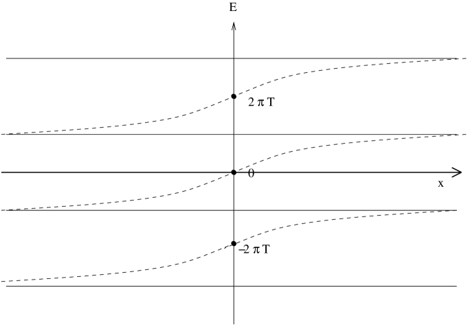
Figure 8: Behaviour of the half-integer gluino energies due the presence of a magnetic flux. Vertical axis is energy in units of $2\pi T$, horizontal axis is the x-axis, orthogonal to the magnetic flux in the y-direction at x=0 (see fig. (2 .b). Gluinos are anti-periodic in the short spatial direction $\tau$, and have zero momentum in x and y direction, as in eq.(95). The continuity of the derivatives at the jump at x=0 is manifest.

We mention as a curiosity the contribution from the potential to the tension: for gluodynamics it is from eq. (93) $5/2$, and for ${\cal N}=1,2,4$ it is given by ${\delta-2\over 2}5$. In the case of gluodynamics this is already true on the level of the effective potential, eq. (41), for any value of q as in eq. (41). In the case of SUSY it is only true for the minimum $\varrho_{k}$ , i.e. only after integration over q.

The kinetic part is subject to ambiguity due to the choice of the running coupling. With our choice the ${\cal O}(g^{2})$ correction is negative and qualitatively like in gluodynamics.

6.1 The profile to lowest order and the fluctuation operator

Up till now we did not look at the other piece of information the effective potential holds in store: the profile corresponding to the tension.

The profile follows from the first term in eq. (89), substituting (39), (33) and (123) and (127). The equation of motion becomes to lowest order in terms of q and $\xi=m_{D}x$, $m_{D}$ the Debye mass from eq. (37):

$$q^{\prime}=q\sqrt{1-{4q\over 3}}$$ (97)

Note that the profile does not depend on k, the strength of the loop, and that this equation is valid for $0<q<1/2$. Continuity of the kinetic term and symmetry arguments extend it to the upper half of the interval. Clearly the profile is for small q exponentially decreasing as $\exp(-m_{D}|x|)$.

The solution for the profile is:

$$q_{m}={3\over 4}(1-\tanh^{2}(-3m_{D}x/8+x_{0}))$$ (98)

with $x_{0}$ such that $q(0)=1/2$.

The ${\cal O}(g^{2})$ correction to the profile is straightforward as long as we stay away from its wings (small q). The reason is the pole at q=0 in the kinetic term. This pole signals the well-known presence of corrections to the Debye mass which are not ${\cal O}(g^{2})$, but larger, by a logarithmic amount. In ref. [19] this problem is discussed in more detail.

A last remark concerns the ${\cal O}(g^{3})$ corrections. They can be obtained from their gluodynamic analogue, as the following argument shows.

The second derivative of the lowest order potential $V_{1}$. It reads:

$$V_{1}^{\prime\prime}(q)=m_{D}^{2}(1-4q).$$ (99)

This turns out to be the one loop self-mass of the time component of a stationary, zero spatial momentum gluon, in the background q. The gluon itself is supposed to be q-neutral, so is not screened by the background. Such gluons are the cause of the familiar, electric infra-red divergencies present in the plasma without background.

The q-independent part of the self-mass gives upon resummation the Debye mass corrected gluon propagator, and hence the $OO(g^{3})$ correction to the free energy:

$$\mbox{Free energy due to soft modes}\sim 1/2\log\det(-\nabla^{2}+m_{D}^{2})\sim m_{D}^{3}\sim g^{3}.$$ (100)

Taking into account the q dependence of the selfmass one computes the same correction but now to the tension $\varrho_{k}$ through the determinant. Since we now compute soft, ${\cal O}(gT)$, fluctuations, which are of the same order as the length scale in the profile the use of gradient expansions is not allowed in this determinant. So one has to evaluate the eigenvalue spectrum of the Schroedinger equation:

$$\mbox{tension due to soft modes}\sim{1\over 2}\log\det\bigg{(}-\nabla^{2}+m_{D}^{2}(1-3/\cosh^{2}(-3m_{D}x/8+x_{0}))\bigg{)}.$$ (101)

However this calculation has already been done in gluodynamics[19], where the fluctuation operator $V^{\prime\prime}_{1}(q_{m})$ is identical, up to some trivial rescalings.

7 Conclusions

In this paper the corrections to the tension of the ’t Hooft loop for hot SUSY theories have been computed to two loop order. The cubic order is shown to be a fairly trivial rescaling of the same problem in gluodynamics. The calculation can be done analytically because the one-dimensional Schroedinger problem, eq. (101), is separable.

What can the understanding of the spatial ’t Hooft loop bring us in terms of a better understanding of the hot phase? After all, the most we learn from it seems to be that it scales according to the Casimir scaling law, $k(N-k)$ and that this scaling law is characteristic for gluons, the screened quasi-particles, being in the adjoint representation. This comes hardly as a surprise.

However, in ${\cal N}=4$ theory the self-duality of the theory at zero temperature may help to shed light on the behaviour of the spatial Wilson loop. The latter measures the mean flux of magnetic quasi-particles . It is well-known from lattice calculations [26] that also the Wilson loops show Casimir scaling. It is tempting to associate to this scaling magnetic quasi-particles in the adjoint representation in some magnetic group [18][22][21] and ${\cal N}=4$ theory seems a setting where one may have a more quantitative grip on these ideas.

8 Acknowledgements

The author thanks Kareljan Schoutens for kindly extending hospitality at the Institute for Theoretical Physics of the University of Amsterdam, and for an inspiring atmosphere, Adi Armoni, Prem Kumar and Jefferson Ridgway for bringing the interest of computing higher order corrections to his attention and for instructive e-mail exchange. He is indebted to Rob Pisarski for his input concerning the double line representation for any finite number of colours. Laurent Lellouch and Vincent Bayle graciously provided the author with computational means. Discussions with Misha Stephanov and Dam Son about the leading term for the tension in 2002 at KITP, Santa Barbara, were quite useful. Incisive remarks by Kostas Bachas and his hospitality at the ENS, Paris, helped understanding the gluino zero-mode problem.

Appendix A: Determinant in mixed x and p representation

In this appendix we elaborate on how to compute the determinant of the d’Alembertian with a background B, where the variation with x does not commute with the corresponding derivative. We suppose the colour degrees of freedom have been diagonalized in the Cartan basis $Q^{ij}$, so that the background $B$ below stands for $B^{ij}=B_{ii}-B_{jj}$.

We start with eq. (43) in the main text and write

$$\mbox{Tr}\log(-D^{2}(\underline{B}))-\mbox{Tr}\log(-D^{2}(B))$$ (102)

for the difference between the non-commuting (underlined background B) and the commuting case ( written as B).

We write:

$$\underline{B}=B(X).$$ (103)

The operator X and the momentum operator in the x-direction have the commutation relation as in eq. (42)

$$[X,P_{x}]=-i$$ (104)

and they act in a Hilberspace spanned by the normalized kets $|x\rangle$, with $X|x\rangle=x|x\rangle$. As in the main text we introduce the eigentime t and write the difference of d’Alembertians as:

$$-\mbox{Tr}\int{dt\over t}\bigg{[}\exp(-t(-D(\underline{B}^{2}))-\exp(-t(-D(B)^{2})\bigg{]}.$$ (105)

The trace becomes in this language ($l_{0}=2\pi Tn$, n integer)

$$\mbox{Tr}~{}\exp\bigg{(}-t((l_{0}+B)^{2}+P_{tr}^{2}+P_{x}^{2})\bigg{)}$$ (106)

$$= T\sum_{n}\int{dl_{tr}^{d-2}\over{(2\pi)^{d-2}}}\mu^{4-d}\int dx\langle x|\exp\bigg{(}-t((l_{0}+B(X))^{2}+l_{tr}^{2}+P_{x}^{2})\bigg{)}|x\rangle.$$

The background field $B(X)=B(x+(X-x))$ is expanded around $B(x)$, the field that commutes with $P_{x}$:

$$B(X)=B(x)+B^{\prime}(x)(X-x)+{1\over 2}B^{\prime\prime}(x)(X-x)^{2}+...$$ (107)

We know already- from the absence of a classical potential term- that every derivative $B^{\prime}(x)={dB(x)\over{dx}}$ counts as a factor $g$, and since we are interested in order $g^{2}$ we neglect the dots.

The matrix element in (106) becomes on substitution of the expansion for $B(X)$ ( we use the notation $2A=((l_{0}+B(x)))^{2})^{\prime}$ and $\Omega=A^{\prime}$:

$$\langle x|\exp(-t(l_{0}+B(X))^{2}+l_{tr}^{2}+P_{x}^{2}))|x\rangle$$ (108)

$$= \langle x|\exp(-t(l_{0}+B(x))^{2}+\Omega(X-x-{A\over{\Omega^{2}}})^{2}-{A^{2}\over{\Omega^{2}}}+l_{tr}^{2}+P_{x}^{2}))|x\rangle$$

$$= \langle{A\over{\Omega^{2}}}|\exp(-t(l_{0}+B(x))^{2}+\Omega(X)^{2}-{A^{2}\over{\Omega^{2}}}+l_{tr}^{2}+P_{x}^{2}))|{A\over{\Omega^{2}}}\rangle.$$

The dependence on x in the last expression has been translated away. It stays only implicitely in $B(x)$.

In what follows we assume it makes sense to expand the integral (106) in terms of A and $\Omega$.

We note that in case $\Omega=0$ the matrix element becomes proportional to:

$$\langle x|\exp(-tP_{x}^{2})|x\rangle={1\over{(4\pi t)^{1\over 2}}}.$$ (109)

This is precisely the result one would get from the $l_{x}$ integration, pretending the background is constant.

In our case however we have $\Omega={\cal O}(g^{2})$ and borrow a formula from [23] to take its presence into account:

$$\langle{A\over{\Omega^{2}}}||\exp(-t(\Omega X^{2}+P_{x}^{2}))|{A\over{\Omega^{2}}}\rangle={a^{1\over 2}\over{(4\pi t)^{1\over 2}}}\exp\bigg{(}-{a\over{2t}}{A^{2}\over{\Omega^{4}}}(-1+\cosh\omega)\bigg{)}$$ (110)

with

$$a = {\omega\over{\sinh\omega}}$$ (111)

$$\omega = 2\Omega t.$$ (112)

In the second term expand a and $\cosh\omega$ for small $\omega$ and substitute the result in (108). Terms with $\Omega$ can be transformed

$$\int dx\exp(-t(l_{0}+B(x))^{2})\Omega=\int\exp(-t(l_{0}+B(x))^{2})2A^{2}t$$ (113)

through partial integration in x and the definition of A and $\Omega$ above eq. (108). The boundary terms at $x=\pm\infty$ cancel with each other for $B(\pm\infty)=0,~{}\mbox{or}~{}2\pi T$ after summing over all n in $l_{0}=2\pi nT$. The summation over Matsubara modes introduces the periodicity in B mod $2\pi T$, hence the cancellation.

The result of this expansion becomes for the matrix element in (112) simply:

$$\langle{A\over{\Omega^{2}}}|\exp(-t(\Omega X^{2}+P_{x}^{2}))|{A\over{\Omega^{2}}}\rangle={1\over{(4\pi t)^{1\over 2}}}(1-{1\over 3}A^{2}t^{3}+..).$$ (114)

Looking back at eq. (106) we see that the integrations over $l_{tr}$ produce a power of eigentime $T^{{2-d\over 2}}$. Together with the powers of t coming from the expansion in the oscillator frequency $\Omega$ above , i.e. $t^{3\over 2}$, one arrives at a power $t^{5-d\over 2}$.

This power ensures that the term with the factor $A^{2}=(l_{0}+B(x))^{2}B^{\prime 2}$ becomes, after substitution into (105), through partial integration in the eigentime t:

$$A^{2}={(5-d)\over{2t}}B^{\prime 2},$$ (115)

hence our final result for (102) becomes, using (105), (114) and (115) :

$$\mbox{Tr}\log(-D^{2}(\underline{B}))-\mbox{Tr}\log(-D^{2}(B))$$ (116)

$$= {1\over 3}\int dx~{}B^{\prime 2}{1\over{(4\pi)^{2}}}\bigg{(}{T\over{\mu}}\bigg{)}^{-2\epsilon}{5-d\over 2}{\Gamma({5-d\over 2})\over{\pi^{{5-d\over 2}}}}\sum_{n}{1\over{|n+q|^{5-d}}}.$$

We wrote $q=B(x)/2\pi T$, and $\epsilon=2-d/2$, and to complete the result we take from [24] for $d\rightarrow 4$:

$$\sum_{n}{1\over{|n+q|^{5-d}}}={1\over{\epsilon}}-\psi(q)-\psi(1-q).$$ (117)

The $\psi$ function is the logarithmic derivative of the Euler $\Gamma$ function. It has a simple pole at $q=0$.

In the main text ( eq. (43) and (46) ) expressions of the form:

$$\mbox{Tr}\log(-D^{2}(\underline{B})\pm B^{\prime})-\mbox{Tr}\log(-D(B))$$ (118)

appear.

Expanding the B’ gives us for half the sum of the terms with plus and minus sign:

$$\int dx{B^{\prime 2}\over 2}\mbox{Tr}{-1\over{(-D(B))^{2}}}+\mbox{Tr}\log(-D(\underline{B})^{2})-\mbox{Tr}\log(-D(B)^{2}$$ (119)

By the same technique the first term leads to eq. (116), with the factor ${1\over 3}{5-d\over 2}$ replaced by $-{1\over 2}$.

The difference between boson respectively fermion trace is the periodicity respectively the anti-periodicity. Hence it comes into play in the argument of the $\psi$ functions. For bosons the argument is $q$, for fermions $q+{1\over 2}$.

The former produce a pole at $q=0$, the latter a pole at $q=1/2$, as discussed in the main text. Both these poles signal the presence of infra-red effects, but are remedied in different ways.

Appendix B: Bernoulli polynomials

They are related to the polynomials defined in (32):

$$\hat{B}_{d=4}(x) = {2\over 3}\pi^{2}T^{4}B_{4}(x)$$ (120)

$$\hat{B}_{3}(x) = {2\over 3}\pi T^{3}B_{3}(x)$$ (121)

$$\hat{B}_{2}(x) = {1\over 2}T^{2}B_{2}(x)$$ (122)

$$\hat{B}_{1}(x) = -{T\over{4\pi}}B_{1}(x)$$ (123)

and finally ($\varepsilon(x)$ is the sign function):

$$B_{4}(x) = x^{2}(1-|x|)^{2}$$ (124)

$$B_{3}(x) = x^{3}-{3\over 2}\varepsilon(x)x^{2}+{1\over 2}x$$ (125)

$$B_{2}(x) = x^{2}-\varepsilon(x)x+{1\over 6}$$ (126)

$$B_{1}(x) = x-{1\over 2}\varepsilon(x)$$ (127)

Appendix C: Spinor projectors in $\delta$ dimensions

We establish the form of projectors on Majorana-Weyl spinors in 10 dimensions, on Weyl spinors in 6 dimensions and Majorana spinors in 4 dimensions. This is important for establishing the dimensional factors in the fermion amplitudes.
$\bullet$$\delta=10$. The projector ${\bf 1}_{f}=\lambda\bar{\lambda}$ is defined by $\bar{\lambda}=\lambda^{T}{\bf C}$ and $\Gamma_{11}\lambda=\lambda$.
$\bullet$ $\delta=6$.The projector is defined by $\Gamma_{7}\lambda=\lambda$
$\bullet$ $\delta=4$. The projector is defined by $\bar{\lambda}=\lambda^{T}{\bf C}$
In all these cases one has $\mbox{Tr}\Gamma_{0x}{\bf 1}_{f}=\delta-2$.

Appendix D: Individual diagrams contributing to the potential

We compute the potential term $V=V_{1}+\tilde{g}^{2}V_{2}$ in the effective action:

$$U=\int dx\bigg{[}K(q)q^{\prime 2}+V(q)\bigg{]}.$$ (128)

We refer to fig. (3) and compute in Feynman gauge. All two-loop results below are given in terms og the ’t Hooft coupling $\tilde{g}^{2}=g^{2}N$. The hatted Bernoulli polynomials are given in Appendix B.

We get for the bosonic graphs (a):

$$a_{1} = {\delta\over 2}2k(N-k)\hat{B}_{4}(q)$$

$$a_{2} = -{3\over 4}(\delta-1)k(N-k)\bigg{(}\hat{B}_{2}(q)^{2}+2\hat{B}_{2}(q)\hat{B}_{2}(0)\bigg{)}$$

$$a_{3} = {1\over 4}\delta(\delta-1)k(N-k)\bigg{(}\hat{B}_{2}(q)^{2}+2\hat{B}_{2}(q)\hat{B}_{2}(0)\bigg{)}.$$ (129)

For the ghost graphs (c):

$$c_{1} = -2k(N-k)\hat{B}_{4}(q)$$

$$c_{2} = {1\over 4}k(N-k)\bigg{(}\hat{B}_{2}(q)^{2}+2\hat{B}_{2}(q)\hat{B}_{2}(0)\bigg{)}.$$ (130)

For the one loop fermion and mixed boson-fermion graphs ($q_{f}=q+1/2$):

$$b_{1} = -{\delta-2\over 2}2k(N-k)\hat{B}_{4}(q_{f})$$

$$b_{2} = \bigg{(}{\delta-2\over 2}\bigg{)}^{2}k(N-k)\bigg{[}\hat{B}_{2}(q_{f})^{2}+2\hat{B}_{2}(1/2)\hat{B}_{2}(q_{f})$$ (131)

$$- 2\bigg{(}\hat{B}_{2}(q_{f})\hat{B}_{2}(q)+\hat{B}_{2}(1/2)\hat{B}_{2}(q)+\hat{B}_{2}(0)\hat{B}_{2}(q_{f})\bigg{)}\bigg{]}$$

Compare to eq. (39) and (33) in the main text. Adding $a_{1},b_{1}$ and $c_{1}$ gives $V_{1}$ . $V_{2}$ is obtained by adding $a_{2},a_{3},b_{2}$ and $c_{2}$.

References

- [1] R. D. Pisarski, Invited talk at LAT2008, Williamsburg, Virginia, arXiv:0810.4548.
- [2] G.’t Hooft, Nucl.Phys B138, 1(1978).
- [3] C. P. Korthals Altes, A. Kovner, M. Stephanov, Phys. Lett. B 469 (1999), 205; hep-ph/9909516
-
[4]
N. Weiss, Phys. Rev. D 24,475 (1981); Phys. Rev. D 25 2667 (1982).
D. J. Gross, R. D. Pisarski, L. G. Yaffe, Rev. Mod. Phys. 53, 43 (1981) - [5] L. Brink, J.H. Schwarz and J. Scherk, Nucl.Phys. B121(1977), 77.
- [6] J. de Boer, V. E. Hubeny, M. Rangamani, M.Shigemori, arXiv:0812.5112[hep-th].
- [7] K. Kajantie, M. Laine, K. Rummukainen,Y. Schroeder, Phys.Rev. D 67, 105008, 2003; hep-ph/0211321.
- [8] T. Bhattacharya, A. Gocksch, C. P. Korthals Altes, R. D. Pisarski, Phys.Rev.Lett 66 (1991), 998; Nucl Phys. B 383 (1992), 497.
- [9] A. Gocksch, R. D. Pisarski, Nucl. Phys.B 402, 657 (1993); hep-ph/9302233.
- [10] A. Fotopoulos, T. R. Taylor, Phys. Rev. D 59,061701 (1999); hep-th/9811224.
- [11] C. Kim, S. Rey, Nucl. Phys B564, 430,2000; hep-th/9905205.
- [12] A. Nieto, M. Tytgat, hep-th/9906147v1.
- [13] M.A. Vasquez-Mozo, Phys. Rev. D 60 106010; hep-th/9905030.
- [14] R. D. Pisarski, Phys. Rev D62 (2000), 111501, hep-ph/0006205. P. Bialas, A. Morel, B. Peterson, Nucl. Phys. B707 (2005), 208, hep-lat/0409027. R. D. Pisarski, Phys. Rev D74 (2006),121703, hep-ph/0608242. A. Vuorinen, L. G. Yaffe, Phys. Rev. D74 ( 2006), 025011, hep-ph/0604100.
- [15] R. Jackiw, C. Rebbi, Phys.Rev D13, 3398 (1976).
- [16] A. Armoni, S.P. Kumar. J. Ridgway, JHEP 0901:076, 2009; arXiv:0812.0773 v3.
- [17] P. de Forcrand, B. Lucini, D. Noth, PoS LAT 2005:323, 2006, hep-lat/0510081. F. Bursa, M. Teper, JHEP 0508:060, 2005, hep-lat/0505025.
- [18] P. Giovannangeli, C. P. Korthals Altes, Nucl. Phys.B 608, 203, 2001; hep-ph/0102022.
- [19] P. Giovannangeli, C. P. Korthals Altes, Nucl. Phys. B 721, 1 (2005); hep-ph/0212298.
- [20] C. P. Korthals Altes, Nucl. Phys.B 429, 637,(1994); hep-th/9310195.
- [21] C. P. Korthals Altes, in Erice 2002, ”From quarks and gluons to quantum gravity”, A. Zichichi ed., Plenum Press; Acta Phys. Polon.B34, 5825, 2003; hep-ph/0308229, hep-ph/0406138..
- [22] C. P. Korthals Altes and H. B. Meyer, hep-ph/0509018.
- [23] J. Iliopoulos, C. Itzykson, A. Martin, Rev. Mod. Phys. 47, 165 (1975).
- [24] I. S. Gradshteyn, I. M. Ryzhik, Table of Integrals, Series and Products, Sixth Edition, 2000, Academic Press.
- [25] V. M. Belyaev, I. I. Kogan, Mod. Phys. Lett. A7, (1992),117; C. P. Korthals Altes, M. Laine, Phys. Lett. B511, 269 (2001), hep-ph/0104031; K. Farakos, P. de Forcrand, C. P. Korthals Altes, M. Laine, Nucl. Phys. B 655, 170, 2003; hep-ph/0207343.
- [26] B. Lucini, M. Teper, U. Wenger, JHEP 0406:012, 2004; hep-lat/0404008.
- [27] P. di Vecchia, hep-th/9908148.