First Principle Simulations of Heavy Fermion Cerium Compounds Based on the Kondo Lattice

Abstract

We propose a new framework for first–principle calculations of heavy–fermion materials. These are described in terms of the Kondo lattice Hamiltonian with the parameters extracted from a realistic density functional based calculation which is then solved using continuous–time quantum Monte Carlo method and dynamical mean field theory. As an example, we show our results for the Néel temperatures of Cerium–122 compounds (CeX₂Si₂ with X=Ru, Rh, Pd, Cu, Ag, and Au) where the general trend around the magnetic quantum critical point is successfully reproduced. Our results are organized on a universal Doniach phase diagram in a semi–quantitative way.

First–principle description of heavy–fermion materials has been a challenging problem for a long time. The difficulty arises from the dual nature of the electrons between localization and itinerancy due to the large Coulomb repulsion energy $U$ at each site of the lattice. Here the relatively well–localized f–electrons interact with the itinerant s,p,d–electrons that form the conduction band. The heavy–fermion systems are generally described as the Anderson impurity model in the dilute limit anderson_1961 or the Anderson lattice model (ALM) in the dense limit, and the first–principle description ofthem has been done by several authors han_1997 ; zoelfl_2001 ; held_2001 ; shim_2007 . With the development of dynamical mean field theory (DMFT) georges_1996 and novel continuous–time quantum Monte Carlo (CT–QMC) solvers for the impurity problem rubtsov_2005 ; werner_2006 ; haule_2007 , the ALM description has become quite successful except for a very low temperature range. The numerically exact treatment of the Anderson impurity problem is still very expensive if the temperature range of $O(1)$ K is to be reached. Thus, the first–principle description of strongly–correlated materials around the quantum critical point (QCP) sachdev_1999 , which has recently been attracting a lot of research interest is yet to be solved.

Here we attack the problem using the Kondo lattice model (KLM)trying to focus on the low–energy physics of the ALM. We show how this new approach works for a archetypical family of so called Cerium 122 compounds, CeX₂Si₂ (X=Ru, Rh, Pd, Cu, Ag, and Au), which has been one of the most extensively studied strongly–correlated materials since the discovery of heavy–fermion superconductor CeCu₂Si₂ steglich_1979 . Strictly speaking, we deal with the Coqblin–Schrieffer model coqblin_1969 with full $14$ fold degenerate f–shell but effectively the degeneracy is lowered due to the spin–orbit and crystal–field splittings. With the localized Kondo–impurity picture we can save the amount of the degrees of freedom in our model by eliminating charge fluctuations, and we can reach much lower temperature range as compared to the ALM simulations. The conduction band in the model is given by the hybridization function between the localized 4f orbitals and the s,p,d–conduction bands calculated by the first–principle electronic structure calculation based on the local–density approximation (LDA) with Hubbard I sergey type of the self–energy for the f electrons. Then the Kondo coupling is defined via the Schrieffer–Wolff transformation schrieffer_1966 , and the KLM is solved with the new efficient CT–QMC Kondo impurity solver otsuki_2007 combined with DMFT.

Now we define the realistic KLM Hamiltonian for a given Cerium compound. The general Coqblin–Schrieffer Hamiltonian is the following.

$$\mathcal{H}=\sum_{k}\epsilon_{k}c_{k}^{{\dagger}}c_{k}+J_{\mathrm{K}}\sum_{i\alpha\alpha^{\prime}}f_{i\alpha}^{{\dagger}}f_{i\alpha^{\prime}}c_{i\alpha^{\prime}}^{{\dagger}}c_{i\alpha}+\sum_{i\alpha}\Delta^{\alpha}_{\rm splitting}f_{i\alpha}^{{\dagger}}f_{i\alpha},$$ (1)

Here $\epsilon_{k}$ is the conduction band, $J_{\mathrm{K}}$ is the Kondo coupling, $\Delta^{\alpha}_{\rm splitting}$ is the crystal and spin–orbital field, $c_{k}$ and $f_{i\alpha}$ are the annihilation operators for the conduction and 4f electrons, respectively, with the orbital $\alpha$ on the lattice site $i$. To solve this Hamiltonian we first need to define $J_{\mathrm{K}}$ and the conduction electron Green function. For this we perform the first principle DFT calculation within the local density approximation for s,p,d electrons plus the Hubbard I approximation for the f electrons based on the full–potential linearized muffin–tin orbitals (LMTO) method sergey and calculate the hybridization function han_1997 $\Im\Delta_{\alpha}(\epsilon)=\pi\sum_{k}|V_{\alpha k}|^{2}\delta(\epsilon-\epsilon_{k})\simeq\pi|V_{\alpha}|^{2}\rho(\epsilon)$ where $V_{\alpha k}$ is the hybridization matrix element and $\rho(\epsilon)$ is the density of states of the conduction electrons at energy $\epsilon$ which we measure from the Fermi energy. We use experimental lattice parameters for all materials that we study.

The calculated ${\rm Tr}\Im\Delta(\epsilon)/(\pi N_{\rm F})\equiv[1/(\pi N_{\rm F})]\sum_{\alpha=1}^{N_{\rm F}}\Im\Delta_{\alpha}(\epsilon)$ is shown in Fig. 1 for several representative CeX₂Si₂ materials with X=Ru, Rh, Pd, and Ag. Here $N_{\mathrm{F}}=14$ is the total number of degeneracy and the trace of $\Im\Delta$ is taken over all of $N_{\mathrm{F}}$ states. We note that $\Im\Delta$ shows strong frequency dependence therefore in order to define $J_{\mathrm{K}}$ an averaging over some frequency intervals needs to be performed.

The Kondo coupling $J_{\mathrm{K}}$ is defined by the Schrieffer–Wolff transformation schrieffer_1966 ; muehlschlegel_1968 as follows

$$J_{\mathrm{K}}=\frac{1}{\pi}\int_{-D_{\mathrm{cutoff}}}^{D_{\mathrm{cutoff}}}d\,\epsilon\frac{\mathrm{Tr}\Im\Delta(\epsilon)}{N_{\mathrm{F}}}\left(\frac{1}{|\epsilon_{\mathrm{f}}|}+\frac{1}{(\epsilon_{\mathrm{f}}+U_{\mathrm{eff}})}\right).$$ (2)

Here $\epsilon_{\mathrm{f}}$ is the location of the energy level of 4f orbital, and $U_{\mathrm{eff}}=U-J_{\mathrm{Hund}}$ is the effective on–site Coulomb repulsion taking into account an effective Hund coupling $J_{\mathrm{Hund}}$ that works in the virtual f² state. We set $\epsilon_{\mathrm{f}}=-2.5\mbox{[eV]}$ and $U=5\mbox{[eV]}$ which is a typical value for Cerium compounds. The Hund coupling $J_{\mathrm{Hund}}$ is explored around a realistic value $1$ eV as is explained below. In the present formulation, $U_{\mathrm{eff}}$ incorporates all of the possible multiplet effects in the virtual f² states and some systematic error comes in from the setting of this value, but it is small enough to see the general trend between the materials in the realistic Doniach phase diagram that is obtained in Fig. 4 in the end. Here we have a band cutoff $D_{\mathrm{cutoff}}$ set to be $5$ [eV] which is large enough to make a universal description of the low–energy physics andrei_1983 .

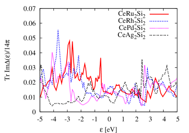
Figure 1: (Color online) The hybridization function $\mathrm{Tr}\Im\Delta(\epsilon)/14$ between the conduction band and the $4f$–electrons calculated by LDA + Hubbard I for CeX₂Si₂ with X=Ru, Rh, Pd, and Ag. The origin of the energy is set to be the Fermi level.

The portion of the conduction electron Green function $G_{\alpha}(\epsilon)$ which has non–zero hybridization with the f–electrons is also proportional to $\Delta_{\alpha}(\epsilon).$ We define the normalized and Hilbert–transformed $G_{\alpha}(i\omega)$ as follows

$$G_{\alpha}(i\omega)=\int_{-D_{\mathrm{cutoff}}}^{D_{\mathrm{cutoff}}}d\,\epsilon\frac{\Im\Delta_{\alpha}(\epsilon)}{i\omega-\epsilon}/\int_{-D_{\mathrm{cutoff}}}^{D_{\mathrm{cutoff}}}d\,\epsilon\Im\Delta_{\alpha}(\epsilon).$$ (3)

The Eqs. (2), (3) provide necessary inputs which are plugged into the CT–QMC and solved with DMFT self–consistency loop. The details of the CT–QMC algorithm for the Coqblin–Schrieffer model are given in otsuki_2007 . These definitions for the realistic model are designed in such a way that it becomes exact in the limit of constant hybridization with the relevant quantity $N_{\mathrm{F}}J_{\mathrm{K}}\rho(0)$ that determines the behavior of the KLM otsuki_2007 .

The LDA results for $N_{\mathrm{F}}J_{\mathrm{K}}\rho(0)$ for the target materials are given in Table 1. The level splittings $\Delta_{\alpha}$ appeared in 1 are implemented as the difference of the positions of $\epsilon_{\mathrm{f}}$’s which are used in the update probability as is described in Ref. otsuki_2007 . These level splittings are taken from the literature and summarized in Table 1. We checked that our results for the Néel temperatures are robust against small changes of factor of $O(1)$ on the level splittings. These $\Delta_{\alpha}$ reduce the effective degeneracy close to $N_{\mathrm{F}}=2$ note_N_F . Thus we call our model “realistic Kondo”lattice instead of the Coqblin–Schrieffer lattice even though we are actually doing the multi–orbital model.

Table 1: Inputs (given by LDA and experiments in the literature) and outputs for each material. $\Delta_{\rm spin-orbit}$ is spin-orbit splitting between $j=5/2$ and $j=7/2$ states. Crystal field splitting of $j=5/2$ state produces three doublets with energy $E_{0}<E_{1}<E_{2}$ with $E_{1}-E_{0}=\Delta_{\rm splitting}^{1}$ and $E_{2}-E_{0}=\Delta_{\rm splitting}^{2}$. $J_{\rm Hund}\sim$ 1 eV is used. The $\Delta_{\rm splitting}^{1},\Delta_{\rm splitting}^{2},\Delta_{\rm splitting}^{\rm spin-orbit}$ are given in meV unit and $T_{\rm N}$ in K. Similar values for the level splittings were used in a recent work vildosola_2005 .

material	$N_{\rm F}J_{\rm K}\rho(0)$	$\Delta_{\rm splitting}^{1}$	$\Delta_{\rm splitting}^{2}$	$\Delta_{\rm splitting}^{\rm spin-orbit}$	$T_{\rm N}$(literature)	$T_{\rm N}$(our results)
CeRu2Si2	0.144	19a,b	34a,b	$\sim 300$	(paramagnetic)h	$0$
CeRh2Si2	0.180	26.7c	58.7c	$\sim 300$	$36$–$39$h	$\sim 70$
CePd2Si2	0.140	19d,e	24d,e	230d	$10$h	$\sim 50$
CeCu2Si2	0.146	32b,f,g	37b,f,g	$\sim 300$	(paramagnetic)h	$\sim 70$
CeAg2Si2	0.110	8.8e	18.0e	$\sim 300$	$8$–$10$h	$\sim 30$
CeAu2Si2	0.125	16.5e	20.9e	$\sim 300$	$8$–$10$h	$\sim 50$

^a Ref. zwicknagl_1992 ^b Ref. ehm_2007 ^c Ref. settai_1997 ^dRef. hansmann_2008 ^eRef. severing_1989 ^fRef. goremychkin_1993 ^gRef. note_crystal_field_CeCu2Si2 ^hRef. endstra_1993

We apply the above framework for the KLM description of CeX₂Si₂ with X=Ru, Rh, Pd, Cu, Au, Ag. We do the following analyses with several settings of $U_{\mathrm{eff}}=U-J_{\mathrm{Hund}}$ for $0\leq J_{\mathrm{Hund}}\overset{<}{\sim}1\$eV for each of the material. For a given material and given parameter set, we determine the Néel temperature by looking at the temperature dependence of staggered susceptibility and locating at which temperature it diverges. Here we follow the formalism of DMFT for the localized f–electron systems as given in otsuki_2009_formalism and use the same method as was utilized for model calculations in otsuki_2009_Doniach . Regarding the realistic input of the Green’s function as is depicted in Fig. 1 , we make an approximation in the calculation of the staggered magnetic susceptibility for the 4f–electrons by decoupling the two–particle density of states $\rho(\epsilon_{1},\epsilon_{2})=\delta(\epsilon_{1}+\epsilon_{2})\rho(\epsilon_{1})$ as if there is a nesting property which becomes exact when the 4f–electrons are on a hypercubic lattice. Thus the tendency to the antiferromagnetic order would be overestimated in addition to having the infinite–dimensional nature in the DMFT solution to the lattice problem. The data specific to CeRh₂Si₂ with which we determine the Néel temperatures for several settings of $J_{\mathrm{Hund}}$ are shown in Fig. 2. In this way for each of the material we look at the magnetic phase transitions for several $J_{\mathrm{K}}$’s by varying corresponding $J_{\mathrm{Hund}}$’s.

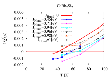
Figure 2: (Color online) Determination of Néel temperatures for several settings of the Hund coupling $J_{\mathrm{Hund}}$. We see that the Néel temperature disappears at the point where $J_{\mathrm{Hund}}$ takes the value between $0.96$ and $0.98$ eV.

As was first discussed by Doniach doniach_1977 ; doniach_1987 and subsequently by many authors, Kondo lattices have two representative energy scales, namely the magnetic ordering energy that is proportional to $(J_{\mathrm{K}}/N_{\mathrm{F}})^{2}\rho(0)$ and the Kondo screening energy which behaves like $\exp\left(-1/N_{\mathrm{F}}J_{\mathrm{K}}\rho(0)\right)$. For small $J_{\mathrm{K}}$’s the former wins but as $J_{\mathrm{K}}$ becomes larger the exponential growth of the latter dominates at some point. Thus a given system can realize in either magnetically ordered phase or non–magnetic Kondo–screened phase. Between these two phases at zero temperature there is thought to be a QCP. We explore this Doniach phase diagram for each material and find the material–specific QCP. We take the data with the setting $J_{\mathrm{Hund}}=0.94$ eV as our realistic result for each material as this strength of the Hund coupling is close to the realistic value and also gives reasonable trend over all materials in the family. Thus obtained Doniach phase diagrams for all of the materials are shown in Fig. 3.

(a)

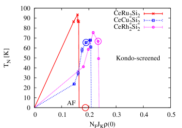
(b)

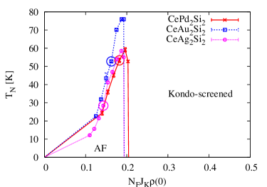
Figure 3: (Color online) Material specific Doniach phase diagrams for CeX₂Si₂ with (a) X=Ru,Cu, and Rh and with (b) X=Pd, Au, and Ag. The realistic results with $J_{\mathrm{Hund}}=0.94$ eV are marked with the larger plot symbols.

Now we can plot all of the six materials CeX₂Si₂ (X=Ru,Rh,Pd,Cu,Ag,Au) on the universal Doniach phase diagram in the same spirit as was done by Endstra et al. in 1993 endstra_1993 but with a different horizontal axis. In the material–specific Doniach phase diagrams in Fig. 3, we see that the locations of QCP’s on the $N_{\mathrm{F}}J_{\mathrm{K}}\rho(0)$ are not actually universal yi-feng_2008 . So we measure the distance between the QCP and the material’s realistic location on the horizontal axis, $N_{\mathrm{F}}J_{\mathrm{K}}\rho(0)-N_{\mathrm{F}}J_{\mathrm{K}}\rho(0)|_{\mathrm{QCP}}$, and plot the Néel temperatures with respect to the value of the distance to QCP defined as $t\equiv[N_{\mathrm{F}}J_{\mathrm{K}}\rho(0)-N_{\mathrm{F}}J_{\mathrm{K}}\rho(0)|_{\mathrm{QCP}}]/N_{\mathrm{F}}J_{\mathrm{K}}\rho(0)|_{\mathrm{QCP}}$. The result is shown in Fig. 4. We expect a systematic error bar in the estimation of the value on the horizontal axis especially around the QCP but these possible systematic errors are small enough to discern the locations of CeX₂Si₂ (X=Ag,Au) and CeRh₂Si₂. The antiferromagnet CeRh₂Si₂ and the paramagnet CeCu₂Si₂ are mixed up within the present level of resolution which is manifested by the result that finite Néel temperature is plotted for CeCu₂Si₂ . However, this is actually caused by the proximity of this material to its QCP as can be seen from Fig. 3 . So our numerical result is consistent with the experimental result that CeCu₂Si₂ is a superconductor at ambient pressure and is thought to be close to the QCP.

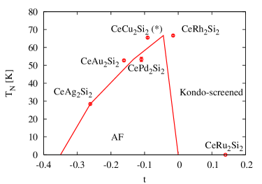
Figure 4: (Color online) Universal Doniach phase diagram for the material family of CeX₂ Si₂. The horizontal axis is defined as follows: $t\equiv[N_{\mathrm{F}}J_{\mathrm{K}}\rho(0)-N_{\mathrm{F}}J_{\mathrm{K}}\rho(0)|_{\mathrm{QCP}}]/N_{\mathrm{F}}J_{\mathrm{K}}\rho(0)|_{\mathrm{QCP}}$. The line is guide for the eye. We plot CeCu₂Si₂ with an asterisk mark to note as it apparently has a finite Néel temperature but that just reflects the result that CeCu₂Si₂ is very close to QCP as can be seen in Fig. 3.

We note that the valence fluctuations which we ignored in our simulation could be important in the realization of the non–magnetic ground state. Indeed it is known that there are some valence fluctuations in CeCu₂Si₂ ansari_1987 and CeRu₂Si₂ yano_2008 . This might make the possible systematic error relatively larger on the right-hand side of our phase diagram holmes_2004 ; otsuki_2009_large_fs . Nevertheless at the present level of description we believe that the realistic KLM works because the number of 4f electrons in Cerium ion is still very close to one ansari_1987 ; yano_2008 . At least for the impurity problem the convergence to the Kondo impurity picture in large $|\epsilon_{\mathrm{f}}|/(\rho(0)V^{2})$ limit of the Anderson model was discussed exactly schlottmann_1984 . Careful comparison between the Anderson lattice and the Kondo lattice regarding the valence fluctuation issue is interesting, especially for CeCu₂Si₂, and further work is ongoing in this direction.

MM thanks Y.–F. Yang, P. Werner, and H. Shishido for helpful discussions and N. Matsumoto for continuous supports. Discussions with the participants in ICAM-DCHEM workshop in August 2008 are acknowledged. This research is supported by NSF Grant No. DMR-0606498 and by DOE SciDAC Grant No. SE-FC02-06ER25793. Numerical computations are performed using TeraGrid supercomputer grant No. 090064.

References

- (1) P. W. Anderson, Phys. Rev. 124, 41 (1961).
- (2) J. E. Han, M. Alouani, and D.L. Cox, Phys. Rev. Lett. 78, 939 (1997).
- (3) M. B. Zölfl, I. A. Nekrasov, Th. Pruschke, V. I. Anisimov, and J. Keller, Phys. Rev. Lett. 87, 276403 (2001).
- (4) K. Held, A. K. McMahan, and R. T. Scalettar, Phys. Rev. Lett. 87, 276404 (2001).
- (5) J. H. Shim, K. Haule, G. Kotliar, Science 318, 1615 (2007).
- (6) A. Georges et al. Rev. Mod. Phys. 68, 13 (1996).
- (7) A. N. Rubtsov, V. V. Savkin, and A. I. Lichtenstein, Phys. Rev. B 72, 035122 (2005).
- (8) P. Werner, A. Comanac, L. de’ Medici, M. Troyer, and A. Millis, Phys. Rev. Lett. 97, 076405 (2006); P. Werner and A. Millis, Phys. Rev. B 74, 155107 (2006).
- (9) K. Haule, Phys. Rev. B 75, 155113 (2007).
- (10) S. Sachdev, Quantum Phase Transitions, Cambridge (1999).
- (11) F. Steglich et al., Phys. Rev. Lett. 43, 1892 (1979).
- (12) B. Coqblin and J. R. Schrieffer, Phys. Rev. 185, 847 (1969).
- (13) For a review, G. Kotliar et. al. Rev. Mod. Phys. 78, 865 (2006).
- (14) J. R. Schrieffer and P. A. Wolff, Phys. Rev. 149, 491 (1966).
- (15) J. Otsuki, H. Kusunose, P. Werner and Y. Kuramoto, J. Phys. Soc. Jpn. 76, 114707 (2007).
- (16) B. Mühlschlegel, Z. Phys. 208, 94 (1968).
- (17) The definition of should always be combined with the cutoff scheme for the conduction band as is discussed in N. Andrei et al., Rev. Mod. Phys. 55, 331 (1983).
- (18) For isotropic KLM the Néel temperature is vanishing small while for the Néel temperature looks unrealistically large otsuki_2009_Doniach . We can observe realistic Néel temperatures when realistic level splittings are introduced.
- (19) J. Otsuki, H. Kusunose, and Y. Kuramoto, J. Phys. Soc. Jpn. 78, 014702 (2009)
- (20) J. Otsuki, H. Kusunose, and Y. Kuramoto, J. Phys. Soc. Jpn. 78, 034719 (2009).
- (21) S. Doniach, Physica B 91, 231 (1977).
- (22) S. Doniach, Phys. Rev. B 35, 1814 (1987).
- (23) Recent update of Doniach phase diagram also discussed this point: Y.-f. Yang et al., Nature 454, 611 (2008). Also the sensitiveness of the quantum critical point to the system-specific features was discussed in V. Yu. Irkhin and M. I. Katsnelson, Phys. Rev. B 56, 8109 (1997).
- (24) P. H. Ansari et al., J. Appl. Phys. 63, 3503 (1987).
- (25) M. Yano et al., Phys. Rev. B 77, 035118 (2008).
- (26) The importance of valence fluctuations in CeCu2Si2 has been discussed in the following paper: A. H. Holmes, D. Jaccard, and K. Miyake, Phys. Rev. B 69, 024508 (2004).
- (27) However both of the Anderson lattice and the Kondo lattice have the large Fermi surface, see, e.g. J. Otsuki, H. Kusunose, and Y. Kuramoto, Phys. Rev. Lett. 102, 017202 (2009), and references therein.
- (28) P. Schlottmann, Z. Phys. B 57, 23 (1984).
- (29) G. Zwicknagl, Adv. Phys. 41, 203 (1992).
- (30) D. Ehm et al. Phys. Rev. B 76, 045117 (2007).
- (31) R. Settai et al. J. Phys. Soc. Jpn. 66, 2260 (1997).
- (32) P. Hansmann et al. Phys. Rev. Lett. 100, 066405 (2008).
- (33) A. Severing et al. Phys. Rev. B 39, 2557 (1989).
- (34) E. A. Goremychkin and R. Osborn, Phys. Rev. B 47, 14280, (1993).
- (35) We note that a crystal–field splitting scheme for CeCu2Si2 mentioned in severing_1989 is obsolete.
- (36) T. Endstra, G. J. Nieuwenhuys, and J. A. Mydosh, Phys. Rev. B 48, 9595 (1993).
- (37) V. Vildosola et al. Phys. Rev. B 71, 184420 (2005).