Radiative corrections to the spectra of heavy particles annihilation into leptons: Dark matter implementation.

Abstract

We calculate the radiative corrections to the annihilation of the Dark Matter particles into leptons. Lepton masses are taken into account. As the Dark Matter particles are considered both Dirac and Majorana fermions. We sum up all the leading logarithms contributions where it is possible. We show that in the Dirac fermion case the resulting cross-section is consistent with the renormalization group prediction: the cross-section have the Drell-Yan form. Whereas, in the Majorana fermions case we have two essentially different limits of the resulting cross-section and quantitively the answer strongly depends on a spectrum of the masses entering the problem.

I Introduction

It is well known fact that approximately quarter of the energy density of our universe belongs to the invisible Dark Matter. The Dark Matter particles are supposed to be neutral heavy particles so we can not observe them in the sky directly. One can detect them through their gravitational influence on the visible matter. But also we can observe the products of the dark matter particles annihilation such as gamma rays, positrons, antiprotons, neutrinos, etc. (so called indirect method of the dark matter detection).

Possible detection of the Dark Matter particles is one of the most exciting problems of the astroparticle physics astro . A lot of experiments have found new phenomena which might be considered as the traces of the new particles experiment . To catch new particles one should know the annihilation cross-section, the distribution of the Dark Matter in the Galactic halo and the model of the propagation of resulting particles from the interaction point to our detectors. Putting aside astrophysical questions we concentrate on the cross-sections calculation.

In particular, in this work we investigate the process of the Dark Matter particles annihilation into the lepton pair with respect to the radiative corrections. We are interested in both the Dirac and Majorana fermions as the Dark Matter candidates. Such a process with respect to the Majorana particles have been calculated in the paper by Bergstrom at al.bergstrom and interesting results have been obtained. It was stated that for the Majorana fermion annihilation the contribution of the next-to-leading order terms can increase the cross-section significantly.

In our calculation we reproduce result bergstrom , investigate dependence on a lepton mass and show the renormalization group structure of this cross-sections.

The paper is organized as follows: after the brief review of the Born cross-sections for the both Dirac and Majorana cases in section [II] we calculate the soft and virtual photon corrections in section [III] and consider the hard photon emission corrections in section [IV] in details. After that in section [V] we demonstrate the Drell-Yan form of the both cross-sections with the large mass of the intermediate particle. We summarise our results and conclusions in the last section [VI].

II Born cross sections

In our calculations we use interaction Lagrangians where $\Psi$ is the electron field and $\chi_{D}$ - the Dirac Dark Matter fermion:

$$\mathcal{L}_{D}^{int}=g_{L}\bar{\Psi}\hat{R}\chi_{D}\phi_{L}+g_{L}^{*}\bar{\chi}_{D}\hat{L}\Psi\phi_{L}^{*}+g_{R}\bar{\Psi}\hat{L}\chi_{D}\phi_{R}+g_{R}^{*}\bar{\chi}_{D}\hat{R}\Psi\phi_{R}^{*},$$

and for Majorana fermion:

$$\mathcal{L}_{M}^{int}=g_{L}\bar{\Psi}\hat{R}\chi_{M}\phi_{L}+g_{L}^{*}\chi_{M}^{T}C\hat{L}\Psi\phi_{L}^{*}+g_{R}\bar{\Psi}\hat{L}\chi_{M}\phi_{R}+g_{R}^{*}\chi_{M}^{T}C\hat{R}\Psi\phi_{R}^{*}.$$ (1)

Here $\chi_{M}$ is the Majorana field, C -the charge conjugation matrix, $\hat{L}=(1-\gamma_{5})/2$, $\hat{R}=(1+\gamma_{5})/2$ - the projection operators and $\phi_{R}$ and $\phi_{L}$ are two different scalar fields. The Lagrangian (1) simulates the part of MSSM Lagrangian mssm i.e. interaction of neutralino ($\chi_{M}$) with electron ($\Psi$ ) and selectron ($\phi_{L,R}$). We suppose, for simplisity, that masses of the scalars $\phi_{R}$ and $\phi_{L}$ (selectrons in MSSM) are identical and equal to $M_{s}$. The Dark Matter particle mass M is less or equal to $M_{s}$.

Further, for simplicity, we put coupling $g_{R}$ to zero. The result for the full Lagrangian will be shown in section [VI].

Fig. 1: The annihilation cross-section of the Majorana particles in the Born approximation

Also, in the light of the MSSM, one can call Majorana fermion neutralino, intermediate scalar particles - sleptons.

At first, let us consider the neutralino annihilation in the Born approximation (Fig.1):

$$\chi_{M}(q_{1})+\chi_{M}(q_{2})\to e^{-}(p_{-})+e^{+}(p_{+}).$$ (2)

Because of indistinguishability of incoming neutralinos one should add the cross graph apart from the direct one (Fig.1). The ”minus” sign goes from the fermionic nature of the neutralinos. There are a lot of papers describing Feynman rules for the Majorana fermions (in different ways), see, for example CHUNG or two , but one can easy write down the matrix element for this process directly using Wick’s theorem. Anyway as a result we have:

$$M_{M}^{B}=M_{direct}-M_{cross}=\frac{|g_{L}|^{2}}{t}\bar{u}(p_{-})\hat{R}u(q_{1})\cdot\bar{v}(q_{2})\hat{L}v(p_{+})-\frac{|g_{L}|^{2}}{\tilde{t}}\bar{u}(p_{-})\hat{R}u(q_{2})\cdot\bar{v}(q_{1})\hat{L}v(p_{+})$$ (3)

Where, as usual, $t=q^{2}-M_{s}^{2}$ and $q=q_{1}-p_{-}=p_{+}-q_{2}$ is the transfered momentum,
correspondingly $\tilde{t}=\tilde{q}^{2}-M_{s}^{2}$, $\tilde{q}=q_{2}-p_{-}=p_{+}-q_{1}$ and $q_{1,2}$ are the four-momenta of the initial particles supposed to be slow (center of mass is implied):

$$q_{1}=(E,P,0,0),\quad q_{2}=(E,-P,0,0),\quad\frac{P}{E}=v\ll 1,\quad q_{1}^{2}=q_{2}^{2}=M^{2},\quad p_{+}^{2}=p_{-}^{2}=m^{2},$$

$$M^{2}\gg m^{2},\quad t=(p_{-}-q_{1})^{2}-M_{s}^{2}=-M^{2}a,\quad a=1+\frac{M_{s}^{2}}{M^{2}},$$ (4)

where $M$ and $M_{s}$ are masses of the incoming and intermediate particles respectively. The Moller factor in the cross sections is assumed to be $I=\sqrt{(q_{1}q_{2})^{2}-M^{4}}=2M^{2}v$ everywhere, (here $v$ is the velocity of the incoming particles in the center-of-mass frame).

We consider the heavy annihilating particles to be almost at rest:

$$q=q_{1}=q_{2}=M(1,0,0,0),\quad p_{\pm}=(E,\pm{\bf p}),\quad E^{2}-{\bf p}^{2}=m^{2},$$

$$E=M,\quad t=\tilde{t}=-M^{2}a.$$ (5)

Using the formulae given in the Appendix we obtain:

$$\frac{1}{4}\sum_{spins}|M_{direct}|^{2}=\frac{1}{4}\sum_{spins}|M_{cross}|^{2}=\frac{|g_{L}|^{4}}{t^{2}}M^{2}E^{2},\quad\frac{1}{4}\sum_{spins}ReM_{direct}M_{cross}^{*}=\frac{|g_{L}|^{4}}{t^{2}}M^{2}(p_{+}p_{-}).$$ (6)

For the squared total matrix element we have:

$$\frac{1}{4}\sum_{spins}|M_{M}^{B}|^{2}=\frac{|g_{L}|^{4}}{a^{2}M^{2}}[2E^{2}-(p_{+}p_{-})]=\frac{m^{2}|g_{L}|^{4}}{a^{2}M^{2}}.$$ (7)

The Born cross-section, respectively:

$$\sigma_{M}^{B}=\frac{\frac{1}{4}\sum|M_{M}^{B}|^{2}\mbox{d}\Gamma_{2}}{4I}=\frac{|g_{L}|^{4}m^{2}}{2^{6}\pi va^{2}M^{4}}.$$ (8)

So, it is the famous result of the cancellation in the Born cross-section of the annihilating Majorana fermions on the small lepton mass gold . This cross-section becomes negligible with lepton as light as the electron.

The Born cross-section for the annihilation of the Dirac particles is rather easy. One need to calculate only one Feynman diagram (Fig.2).

Fig. 2: The annihilation cross-section of the Dirac particles in the Born approximation

$$\sigma^{B}_{D}=\frac{|g_{L}|^{4}}{2^{6}\pi va^{2}M^{2}}.$$ (9)

Here $a=1+(M_{s}^{2}/M^{2})$, where $M$ and $M_{s}$ are the masses of the annihilating and intermediate particles respectively. As one can see, in the case of the annihilation of the Dirac particles there is no suppression on a small lepton mass.

III Contribution from the emission of the virtual and soft real photons

Now, when we have leaned the Born cross sections for the processes, we are interested in the calculation of the perturbative corrections related with the emission of the hard or soft real and virtual photons. In this section we take into account the last two processes which are universal for both Dirac and Majorana cases.

the virtual photons and the counterterms

Among the one-loop Feynman diagrams the main contribution (containing the so-called ”Large Logarithm” terms) arises from the QED type ones. As soon as we provide the calculations in frames of unrenormalized theory we must include the ultraviolet cut-off parameter $\Lambda$, perform the loop integration and take into account the electron and positron wave function counterterms AKHBER :

$$|M^{B}|^{2}\rightarrow|M^{B}|^{2}Z_{e_{-}}Z_{e_{+}},$$ (10)

$$Z_{e_{-}} = Z_{e^{+}}=1-\frac{\alpha}{2\pi}\left[\frac{1}{2}\ln\frac{\Lambda^{2}}{M^{2}}-\ln\frac{m^{2}}{\lambda^{2}}+\frac{1}{2}L+\frac{9}{4}\right]=S_{EW}\left[1-\frac{\alpha}{2\pi}(\frac{1}{2}L-\ln\frac{m^{2}}{\lambda^{2}}+\frac{9}{4})\right],$$

$$S_{EW} = 1-\frac{\alpha}{4\pi}\ln\frac{\Lambda^{2}}{4M^{2}},$$

$$L = \ln\frac{4M^{2}}{m^{2}},$$ (11)

here $\lambda$ is ”photon mass” - small auxiliary parameter which will be dropped away in the final step of the calculations. $L$ is so called ”large logarithm”. The factor $S_{EW}$ will be absorbed by the renormalization of the coupling constant $g$:

$$g^{bare}S_{EW}=g.$$

It results into the counterterms contribution to the cross section:

$$\frac{\sigma^{C}}{\sigma^{B}}=-\frac{\alpha}{\pi}\left[\frac{1}{2}L-\ln\frac{m^{2}}{\lambda^{2}}+\frac{9}{4}\right].$$ (12)

Notice that the contributions arising from the vertex type Feynman diagrams which are shown in Fig.3b and Fig.3c cancel each other due to the different sign of the electron and positron charges.

Fig. 3: The virtual photon correction to the annihilation cross-section

In the calculations of the contribution from the box type Feynman diagram (Fig.3a) one can assume that loop momentum is small compared to the mass of the intermediate particle $|k^{2}|<<M_{s}^{2}$:

$$(q-k)^{2}-M_{s}^{2}\approx t.$$ (13)

In such a way we will have the amplitude corresponding to the triangular Feynman diagram. The part of its contribution which contains the logarithm of the ultra-violet cut-off parameter $\ln(\Lambda^{2}/M^{2})$ will be absorbed as well by the coupling constant renormalization.

Interference of this part of 1-loop corrected amplitude with Born one contains:

$$2M^{B}*M^{box}=-\frac{1}{t^{2}}\frac{\alpha}{2\pi}\int\limits_{0}^{1}dx\int\limits_{0}^{1}\frac{ydy}{d}S_{1}*S_{2},$$ (14)

with $d=y^{2}p_{x}^{2}+(1-y)\lambda^{2},\ p_{x}=xp_{-}-(1-x)p_{+}$ and

$$S_{1}*S_{2}={\rm Tr}\left[\hat{p}_{-}\gamma_{\mu}(\hat{p}_{-}-y\hat{p}_{x})\hat{L}(\hat{Q}_{1}+M)\hat{R}\right]\times$$

$${\rm Tr}\left[(\hat{Q}_{2}-M)\hat{L}(-\hat{p}_{+}-y\hat{p}_{x})\gamma_{\mu}\hat{p}_{+}\hat{R}\right].$$

Integration over the Feynman parameter $y$ can be performed using:

$$\int\limits_{0}^{1}\frac{ydy}{d}=\frac{1}{2p_{x}^{2}}\ln\frac{p_{x}^{2}}{\lambda^{2}};\qquad\int\limits_{0}^{1}\frac{y^{2}dy}{d}=\frac{1}{p_{x}^{2}}.$$ (15)

Here $p_{x}^{2}=m^{2}-sx(1-x)-i0,\ s=(p_{+}+p_{-})^{2}=4M^{2}$ and

$$Re\int\limits_{0}^{1}\frac{1}{p_{x}^{2}}=-\frac{2}{s}L,\quad Re\int\limits_{0}^{1}\frac{1}{p_{x}^{2}}\ln\frac{p_{x}^{2}}{m^{2}}=-\frac{1}{s}[L^{2}-8\xi_{2}],\qquad\xi_{2}=\frac{\pi^{2}}{6},$$ (16)

we obtain:

$$\sigma^{v}=\sigma^{B}\left(-\frac{\alpha}{\pi}\right)\left[\frac{1}{2}(L^{2}-8\xi_{2})+L\ln\frac{m^{2}}{\lambda^{2}}-2L\right].$$ (17)

the soft photon emission

Contribution from the soft photon emission is standard:

$$\frac{\sigma^{soft}}{\sigma^{B}}=\left.-\frac{\alpha}{4\pi}\int\frac{d^{3}k}{\omega}\left(\frac{p_{-}}{p_{-}k}-\frac{p_{+}}{p_{+}k}\right)^{2}\right|_{\omega<\Delta E}.$$

After integation one can obtain:

$$\frac{\sigma^{soft}}{\sigma^{B}}=\frac{\alpha}{\pi}\left[2(L-1)\ln\Delta+(L-1)\ln\frac{m^{2}}{\lambda^{2}}+\frac{1}{2}L^{2}-2\xi_{2}\right],\ \Delta=\frac{\Delta E}{M}<<1.$$ (18)

The sum of the virtual and soft photons emission contributions is free from the infrared divergence (remains finite in limit $\lambda\to 0$), as soon as it does not contain terms with $L^{2}$:

$$\frac{\sigma^{C}+\sigma^{v}+\sigma^{soft}}{\sigma^{B}}=\frac{\alpha}{\pi}\left[(L-1)\left(2\ln\Delta+\frac{3}{2}\right)+2\xi_{2}-\frac{3}{4}\right].$$ (19)

Including the Born cross section the result can be written in form:

$$\frac{\sigma^{B}+\sigma^{C}+\sigma^{v}+\sigma^{soft}}{\sigma^{B}}=\frac{\sigma^{BSV}}{\sigma^{B}}=(1+\beta P_{\Delta})^{2}(1+\frac{\alpha}{\pi}K_{vs}),\qquad K_{vs}=2\xi_{2}-\frac{3}{4},$$ (20)

with $P_{\Delta}=2\ln\Delta+3/2$ is the so called delta-part of the evolution equation kernel $P(x)$ and

$$\beta=\frac{\alpha}{2\pi}(L-1).$$ (21)

IV The hard photon emission

In this section we consider annihilation cross-sections with respect to the hard photon emission, i.e. processes:

$$\chi_{M}(q_{1})+\chi_{M}(q_{2})\to e^{+}(p_{+})+e^{-}(p_{-})+\gamma(k)$$

and $$\chi_{D}(q_{1})+\bar{\chi}_{D}(q_{2})\to e^{+}(p_{+})+e^{-}(p_{-})+\gamma(k),$$

$$\qquad p_{\pm}^{2}=m^{2},\qquad k^{2}=0.$$

The cross-section for a 2$\to$3 process have a form of:

$$d\sigma=\frac{\frac{1}{4}\sum|M^{hard}|^{2}d\Gamma_{3}}{4I},$$ (23)

where the phase volume is:

$$d\Gamma_{3}=\frac{(2\pi)^{4}}{(2\pi)^{9}}\frac{d^{3}p_{+}d^{3}p_{-}d^{3}k}{2E_{+}2E_{-}2\omega}\delta^{4}(q_{1}+q_{2}-p_{+}-p_{-}-k),$$

can be written in the form:

$$d\Gamma_{3}=\frac{M^{2}}{32\pi^{3}}dx_{-}dx_{+}dx\delta(2-x-x_{-}-x_{+}),$$ (24)

with

$$x_{\pm}=E_{\pm}/M,\ x=\omega/M,\ 1-x<x_{\pm}<1-\delta,\ \delta=\frac{m^{2}(1-x)}{4M^{2}x},\ 1<x_{+}+x_{-}<2-\Delta$$ (25)

Here $x>\Delta$ and $\Delta E=M\Delta$ is the minimal value of the photon energy, where the photon can be considered as a hard one.

Majorana case

Let us now calculate hard photon emission for the Majorana cross-section.

Fig. 4: The hard photon emission for the Majorana cross-section

As well as for the Majorana Born cross-section, here we have ”doubling” of the graphs in the matrix element (Fig.4). So, the appropriate matrix element contains 6 gauge invariant Feynman amplitudes:

$$M_{M}^{hard} = -ie(M_{direct}^{hard}-M_{cross}^{hard}),$$

$$M_{direct}^{hard} = |g_{L}|^{2}\left(\frac{1}{t_{-}\chi_{+}}\bar{u}(p_{-})\hat{L}u(q_{1})\cdot\bar{v}(q_{2})\hat{R}(-\hat{p}_{+}-\hat{k}+m)\hat{\varepsilon}v(p_{+})+\right.$$

$$+ \frac{1}{t_{+}\chi_{-}}\bar{u}(p_{-})\hat{\varepsilon}(\hat{p}_{-}+\hat{k}+m)\hat{L}u(q_{1})\bar{v}(q_{2})\hat{R}v(p_{+})+$$

$$+ \left.\frac{(\varepsilon,q_{+}+q_{-})}{t_{+}t_{-}}\bar{u}(p_{-})\hat{L}u(q_{1})\bar{v}(q_{2})\hat{R}v(p_{+})\right),$$

$$M_{cross}^{hard} = M_{direct}^{hard}(t_{\pm}\rightarrow\tilde{t}_{\pm},q_{1}\leftrightarrow q_{2}).$$ (26)

Here and below $t_{\pm}=q_{\pm}^{2}-\tilde{m}^{2}$, where $q_{+}=p_{+}-q_{2},\ q_{-}=q_{1}-p_{-}\$, $\tilde{t}_{\pm}=\tilde{q}_{\pm}^{2}-\tilde{m}^{2}$,
where $\tilde{q}_{+}=p_{+}-q_{1},\ \tilde{q}_{-}=q_{2}-p_{-}$.

Now we need to square this matrix element. It consists of three essentially different parts:
$A_{pole}$ - the part that have poles when $x_{+}$ or $x_{-}$ are equal to 1, $A_{0}$ - part remaining in the zero lepton mass limit and $A_{other}$ - other terms which are insignifficant because of their smallness as we will see later.

$$\frac{1}{4}\sum_{spins}|M_{M}^{hard}|^{2} = A_{pole}+A_{0}+A_{other},$$ (27)

$$A_{pole} = \frac{e^{2}|g_{L}|^{4}m^{2}}{M^{4}}\left(\frac{a+2x_{-}+x_{-}(a+2x_{+})}{2(1-x_{+})\tau_{+}^{2}\tau_{-}}+\frac{a+2x_{+}+x_{+}(a+2x_{-})}{2(1-x_{-})\tau_{+}\tau_{-}^{2}}\right.$$ (28)

$$+ \left.\frac{1}{(1-x_{+})(1-x_{-})\tau_{+}\tau_{-}}-\frac{m^{2}}{4(1-x_{+})^{2}\tau_{+}M^{2}}-\frac{m^{2}}{4(1-x_{-})^{2}\tau_{-}M^{2}}\right).$$

Where $\tau_{\pm}=2(1-x_{\pm})-a$ goes from propogators of the intermediate particle $t_{\pm}=M^{2}\tau_{\pm}$.

$$A_{0}=\frac{4e^{2}|g_{L}|^{4}(1-x)}{M^{2}\tau_{+}^{2}\tau_{-}^{2}}\left[(1-x_{+})^{2}+(1-x_{-})^{2}\right].$$ (29)

As one can see $A_{0}$ does not contain lepton mass, so this term can not be proportional to the Born cross-section for the Majorana particles. The term remains finite in the zero lepton mass limit.

$$A_{other}=\frac{e^{2}|g_{L}|^{4}m^{2}}{2\tau_{+}^{2}\tau_{-}^{2}M^{4}}((\tau_{+}-\tau_{-})^{2}+\tau_{+}^{2}+\tau_{-}^{2}-6(\tau_{+}+\tau_{-})+$$

$$24(x_{+}+x_{-})-16x_{+}x_{-}-24)+O(\frac{m^{4}}{M^{6}}).$$ (30)

In order to explicitly separate pole structure of our result, i.e. future ”Large Logarithms”, we rewrite $A_{pole}+A_{other}=A_{sing}+\tilde{\Phi}_{M}$ with help of the followng identities:

$$\frac{f(x)}{x-x_{0}} = \frac{f(x_{0})}{x-x_{0}}+\frac{f(x)-f(x_{0})}{x-x_{0}},$$

$$\frac{f(x)}{(x-x_{0})^{2}} = \frac{f(x_{0})}{(x-x_{0})^{2}}+\frac{f(x)-f(x_{0})-f^{\prime}(x_{0})(x-x_{0})}{(x-x_{0})^{2}}+O(1),$$ (31)

$$\frac{1}{(1-x_{+})(1-x_{-})}=\frac{1}{x}\left(\frac{1}{1-x_{+}}+\frac{1}{1-x_{-}}\right),\ \mbox{remind that}\ 2=x+x_{+}+x_{-}.$$ (32)

Thus we arrive to the expression:

$$\frac{1}{4}\sum_{spins}|M_{M}^{hard}|^{2} = A_{sing}+A_{0}+\tilde{\Phi}_{M},$$ (33)

$$A_{sing} = \frac{e^{2}|g_{L}|^{4}m^{2}}{2a^{2}M^{4}}\left(\frac{2-2x}{x}-\frac{ax^{2}}{x(2x-a)}\right)\left[\frac{1}{1-x_{+}}+\frac{1}{1-x_{-}}\right]-$$

$$- \frac{e^{2}|g_{L}|^{4}m^{4}}{4a^{2}M^{6}}\left[\frac{1}{(1-x_{+})^{2}}+\frac{1}{(1-x_{-})^{2}}\right].$$

Here $\tilde{\Phi}_{M}$ is the part of so-called K-factor for Majorana case. One can find it the Appendix.

Notice that in the limit of the large intermediate particle mass ($a\gg 2$) one has for singular term:

$$A_{sing}\to A_{\gamma}=\frac{e^{2}|g_{L}|^{4}m^{2}}{2a^{2}M^{4}}\left(\frac{1+(1-x)^{2}}{x}\right)\left[\frac{1}{1-x_{+}}+\frac{1}{1-x_{-}}\right]-$$

$$-\frac{e^{2}|g_{L}|^{4}m^{4}}{4a^{2}M^{6}}\left[\frac{1}{(1-x_{+})^{2}}+\frac{1}{(1-x_{-})^{2}}\right].$$ (35)

So we have two essential limits:

$$\frac{1}{4}\sum_{spins}|M_{M}^{hard}|^{2}=\left\{\begin{array}[]{lr}A_{0},&\ \mu^{2}=\frac{m^{2}}{M^{2}}\ll 1\\ A_{M}^{\gamma}+\tilde{\Phi}_{M},&a\gg 2,\end{array}\right.$$ (36)

or in terms of the differential cross section:

$$\frac{\mbox{d}^{2}\sigma^{hard}_{M}}{\mbox{d}x_{+}\mbox{d}x_{-}}=\left\{\begin{array}[]{lr}F_{0},&\ \mu^{2}\ll 1\\ F_{M}^{\gamma},&a\gg 2,\end{array}\right.$$ (37)

with

$$F_{0}=\frac{\alpha|g_{L}|^{4}(1-x)}{2^{4}\pi^{2}v\tau_{+}^{2}\tau_{-}^{2}M^{2}}\left[(1-x_{+})^{2}+(1-x_{-})^{2}\right],$$ (38)

$$F_{M}^{\gamma}=\sigma_{M}^{B}\frac{\alpha}{\pi}\left\{\left(\frac{1+(1-x)^{2}}{2x}\right)\left[\frac{1}{1-x_{+}}+\frac{1}{1-x_{-}}\right]-\frac{\mu^{2}}{4}\left[\frac{1}{(1-x_{+})^{2}}+\frac{1}{(1-x_{-})^{2}}\right]+\Phi_{M}\right\}.$$ (39)

Here new notations were introduced:

$$\Phi_{M}=\frac{M^{2}a^{2}}{\mu^{2}}\tilde{\Phi}_{M},\qquad\mu=\frac{m}{M}.$$ (40)

Now we are interested in the case of the zero lepton masses. Imagine that we put m = 0 from the beginning. Than Born cross-section is equal to zero ($\sigma_{M}^{B}=0$). There is no emission from $e^{+}$ and $e^{-}$ legs, only from intermediate scalar. Soft real and virtual photon contributions are absent. Then we obtain for double differential cross-section:

$$\frac{\mbox{d}^{2}\sigma_{0}}{\mbox{d}x_{+}\mbox{d}x_{-}}=\frac{\alpha|g_{L}|^{4}(1-x)}{2^{4}\pi^{2}v\tau_{+}^{2}\tau_{-}^{2}M^{2}}\left[(1-x_{+})^{2}+(1-x_{-})^{2}\right]$$ (41)

Integrating over $x_{-}$ one can find:

$$\frac{\mbox{d}\sigma_{0}}{\mbox{d}x_{+}}=\frac{\alpha|g_{L}|^{4}}{2^{8}\pi^{2}va\tau_{+}^{2}M^{2}}\left[2x_{+}(-3a^{2}+ax_{+}-4(1-x_{+})^{2})\right.$$

$$-\left.a(-3a^{2}+4ax_{+}-4(1-x_{+})^{2})\ln\left(\frac{a}{a-2x_{+}}\right)\right].$$ (42)

And performing last integration we receive:

$$\sigma_{0}=\frac{\alpha|g_{L}|^{4}}{2^{7}\pi^{2}vaM^{2}}\left(4a-1-\frac{a((11-4a)a-6)}{2a-2}\ln\left[\frac{a-2}{a}\right]\right.$$

$$+\left.a^{2}\left(\frac{\pi^{2}}{6}-\ln^{2}\left[\frac{a}{2a-2}\right]-2\mathcal{L}i_{2}\left[\frac{a}{2a-2}\right]\right)\right).$$ (43)

Here $\mathcal{L}i_{2}=-\int\limits_{0}^{1}\frac{dt}{t}\ln(1-t)$ is Euler dilogarithm. This result reproduces the one given in the paper by Bergstrom at al.bergstrom .

Dirac case

Matrix element of the hard photon emission in the case of the Dirac annihilating fermions contains only three Feynman diagrams (Fig.5). It is equal to $M_{direct}^{hard}$ written down in (26).

Fig. 5: The hard photon emission for the Dirac cross-section.

Taking the square of the appropriate matrix element and separating singular terms as in previous case we obtain, in total agreement with the general theory KF85 , the following expression:

$$\frac{\mbox{d}^{2}\sigma^{hard}_{D}}{\mbox{d}x_{+}\mbox{d}x_{-}} = \sigma_{B}^{D}\frac{\alpha}{\pi}\left\{\frac{1+(1-x)^{2}}{2x}\left(\frac{1}{1-x_{+}}+\frac{1}{1-x_{-}}\right)\right.$$ (44)

$$- \left.\frac{\mu^{2}}{4}\left(\frac{1}{(1-x_{+})^{2}}+\frac{1}{(1-x_{-})^{2}}\right)+\Phi_{D}(x_{+},x_{-})\right\}.$$

Again,one can find expression for $\Phi_{D}$ in Appendix. As one can see the structure of the differential cross-section in Dirac case (44) is almost the same as one in the Majorana case (37)(in the limit a$\gg$2) up to appropriate Born cross-sections. Introduce value

$$\frac{\mbox{d}^{2}\sigma^{hard}_{i}}{\mbox{d}x_{+}\mbox{d}x_{-}} = \sigma_{i}^{B}\frac{\alpha}{\pi}\left\{\frac{1+(1-x)^{2}}{2x}\left(\frac{1}{1-x_{+}}+\frac{1}{1-x_{-}}\right)\right.$$ (45)

$$- \left.\frac{\mu^{2}}{4}\left(\frac{1}{(1-x_{+})^{2}}+\frac{1}{(1-x_{-})^{2}}\right)+\Phi_{i}(x_{+},x_{-})\right\},$$

where i=D,M is specified Dirac and Majorana cases for the appropriate values. In such a way we can describe both Dirac and Majorana cases simultaneously.

Further integration is straightforward:

$$\int\limits_{1-x_{\mp}}^{1-\delta}dx_{\pm}\left[\frac{\mu^{2}}{(1-x_{\pm})^{2}},\frac{1}{1-x_{\pm}}\right]=\left[\frac{4x_{\mp}}{1-x_{\mp}},L+\ln\frac{x_{\mp}^{2}}{1-x_{\mp}}\right],$$ (46)

$$\quad L=\frac{4}{\mu^{2}},\quad\delta=\frac{\mu^{2}x}{4x_{\mp}},\ 2=x+x_{+}+x_{-},\ \mu=\frac{m}{M}$$

Let us say a few words about the upper limit of the integration. Consider the scalar product of the two four-vectors, for instanse, $(p_{-},k)$. On the one hand:

$$(p_{-},k)=E_{-}\omega-|{\bf p_{-}}||{\bf k}|\cos\theta_{-}\approx M^{2}x_{-}x(1-v_{-}\cos\theta_{-}),$$

$$v_{-}=\frac{|\bf p_{-}|}{E_{-}}=\frac{\sqrt{E_{-}^{2}-m^{2}}}{E_{-}}\approx 1-\frac{m^{2}}{2E_{-}^{2}}=1-\frac{\mu^{2}}{2x_{-}^{2}}.$$ (47)

On the other hand:

$$(p_{-},k)=\frac{1}{2}[(p_{-}+k)^{2}-m^{2}]=\frac{1}{2}[(Q_{1}+Q_{2}-p_{+})^{2}-m^{2}]\approx 2M^{2}(1-x_{+}).$$ (48)

Thus, we have:

$$x_{-}x(1-v_{-}\cos\theta_{-})=2(1-x_{+}),$$ (49)

and from the constraint $\cos\theta_{-}<1$ we obtain

$$x_{+}<1-\delta,\qquad\delta=\frac{\mu^{2}x}{4x_{-}}.$$ (50)

Because in the upper limit of the integration $x_{+}\approx 1$ than $\delta\approx\frac{\mu^{2}(1-x_{-})}{4x_{-}^{2}}$. Similarly, one can obtain constraint on $x_{-}$.

As a result of the integration we have double differential distribution:

$$\frac{d^{2}\sigma_{i}^{hard}}{\sigma_{B}dx_{+}dx_{-}}=\frac{\alpha}{\pi}\left\{\left[\frac{1}{2}\delta(1-x_{+})P_{\theta}(x_{-})+\frac{1}{2}\delta(1-x_{-})P_{\theta}(x_{+})\right](L-1)+K^{h}_{i}(x_{+},x_{-})\right\},$$ (51)

with

$$K_{i}^{h}(x_{+},x_{-})=\frac{1}{2}[\delta(1-x_{+})(1-x_{-}+\frac{1+x_{-}^{2}}{1-x_{-}}\ln\frac{x_{-}^{2}}{1-x_{-}})+$$ (52)

$$\delta(1-x_{-})(1-x_{+}+\frac{1+x_{+}^{2}}{1-x_{+}}\ln\frac{x_{+}^{2}}{1-x_{+}})]+\Phi_{i}(x_{+},x_{-})$$ (53)

and

$$P_{\theta}(z)=\frac{1+z^{2}}{1-z}\theta(1-z-\Delta),\ \Delta=\frac{\Delta E}{M}.$$ (54)

We note that $P_{\theta}(z)$ is the so called $\theta$-part of the evolution equation kernel for the non-singlet of twist-2 operators matrix elements KF85 .

Let us remark here that singularity on lepton mass terms (so-called Large Logarithm which can give essential contribution ) arise from such kinematical region where photon is emitted in the direction close to the charge lepton propogation one.

V Drell-Yan form of the spectrum

Taking into account the contribution from the emission of the hard photon with $x>\Delta E/M$ we obtain KF85 :

$$\frac{d\sigma_{i}}{\sigma_{i}^{B}}=\frac{d\sigma^{BSV}+d\sigma_{i}^{hard}}{\sigma_{i}^{B}}=$$ (56)

$$= D(x_{-},\beta)D(x_{+},\beta)(1+\frac{\alpha}{\pi}K_{i}(x_{+},x_{-}))dx_{+}dx_{-},$$

$$\beta=\frac{\alpha}{2\pi}(L-1),\ L=\ln\frac{4}{\mu^{2}},$$

with the Structure function $D(x,\beta))$:

$$D(x,\beta)=\delta(1-x)+\beta P^{(1)}(x)+\frac{1}{2!}(\beta)^{2}P^{(2)}(x)+...,$$ (57)

and the kernel of evolution equation of twist-2 operators is:

$$P^{(1)}(x)=P(x)=\lim_{\Delta\to 0}[P_{\Delta}\delta(1-x)+P_{\theta}(x)\theta(1-x-\Delta)],$$ (58)

with

$$P^{(n)}(x)=\int\limits_{x}^{1}\frac{dy}{y}P^{(n-1)}(y)P(\frac{x}{y}),n=2,3,....$$ (59)

Kernel $P(x)$ have a property $\int\limits_{0}^{1}P(x)dx=0$, which results in

$$\int\limits_{0}^{1}dxD(x,\beta)=1.$$ (60)

Using previous relation the inclusive distribution on the positron energy fraction can be obtained as:

$$\frac{d\sigma_{i}}{\sigma_{i}^{B}dx_{+}}=D(x_{+},\beta)(1+\frac{\alpha}{\pi}K_{i}(x_{+})).$$ (61)

Photon energy distribution is (from eq.(45))

$$\frac{d\sigma_{i}}{\sigma_{i}^{B}dx}=\int\limits_{0}^{1}dx_{+}\int\limits_{0}^{1}dx_{-}\frac{d^{2}\sigma_{i}^{hard}}{\sigma_{i}^{B}dx_{+}dx_{-}}(1+\frac{\alpha}{\pi}K^{\gamma}_{i}(x))\delta(2-x-x_{+}-x_{-})$$ (62)

The explicit forms of $K_{i}(x_{+})$ and $K^{\gamma}_{i}(x)$ factors are:

$$K_{i}(x_{+}) = \frac{\pi^{2}}{3}-\frac{3}{4}+\frac{1}{2}\left[1-x_{+}+\frac{1+x_{+}^{2}}{1-x_{+}}\ln\frac{x_{+}^{2}}{1-x_{+}}\right]+$$

$$+ \int\limits_{1-x_{+}}^{1}\Phi_{i}(x_{+},x_{-})dx_{-},\ 0<x_{+}<1,$$

$$K^{\gamma}_{i}(x) = \frac{\pi^{2}}{3}-\frac{3}{4}+x+\frac{1+(1-x)^{2}}{x}\ln(1-x)+\int\limits_{1-x}^{1}\Phi_{i}(2-x-x_{-},x_{-})dx_{-}.$$ (65)

For practical calculations the smoothed form of the Structure Function can be useful KF85 :

$$D(x,\beta)=D^{NS}(x,\beta)=2\beta(1-x)^{2\beta-1}[1+\frac{3}{2}\beta]-\beta(1+x)+O(\beta^{2}).$$ (66)

In general the process with two and more electron-positron pairs can be taken into account. It results in the replacement $D^{NS}\to D^{NS}+D^{e^{+}e^{-}}$ (see KF85 ).

VI results and conclusions

In this paper we have considered the Dark Matter particles annihilation into leptons with respect of QED radiative corrections. We have taken into account nonzero leptons masses. In the case of the Dirac incoming fermions the obtained cross-section is in total agreement with the Drell-Yan form. Whereas in the case of the Majorana fermions the form of the answer strongly depends on the mass spectrum of this problem (lepton mass and mass of the intermediate particle). In details the results of our calculation are presented below:
1) Distribution of the differencial cross-section on the positron energy fraction for Dirac case is (eq.(61)):

$$\frac{d\sigma_{D}}{dx_{+}}=\sigma_{D}^{B}D(x_{+},\beta)(1+\frac{\alpha}{\pi}K_{D}(x_{+}))$$ (67)

and for Majorana case is (eqs.(42) and (61)):

$$\frac{\mbox{d}\sigma_{M}}{\mbox{d}x_{+}}=\left\{\begin{array}[]{lr}\frac{\alpha|g_{L}|^{4}}{2^{8}\pi^{2}va\tau_{+}^{2}M^{2}}\Sigma_{M},&\ \mu^{2}\ll 1\\ \sigma_{M}^{B}D(x_{+},\beta)(1+\frac{\alpha}{\pi}K_{M}(x_{+})),&a\gg 2,\end{array}\right.$$ (68)

where

$$\Sigma_{M}=2x_{+}(-3a^{2}+ax_{+}-4(1-x_{+})^{2})-a(-3a^{2}+4ax_{+}-4(1-x_{+})^{2})\ln\left(\frac{a}{a-2x_{+}}\right).$$ (69)

Expression for $d\sigma_{i}$ with the Structure Function $D(x,\beta)$ means that effectively we have summarized leading logarithms in all orders of the perturbation series or, physically, we have taken into account all the photons emmitted from legs (1 photon + 2 photons + 3 photons + …) KF85 .

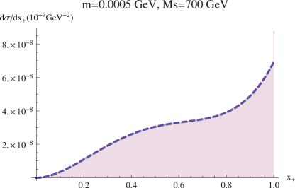
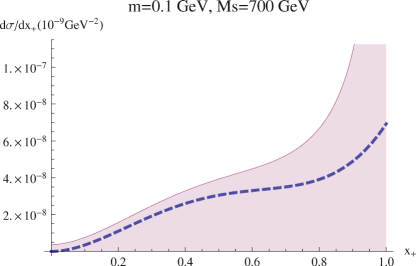
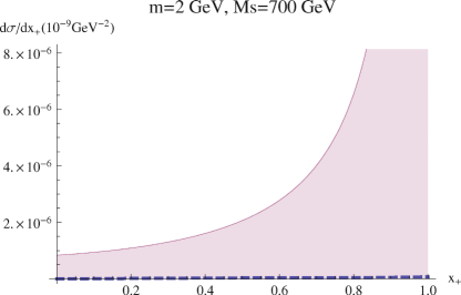
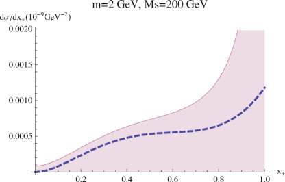
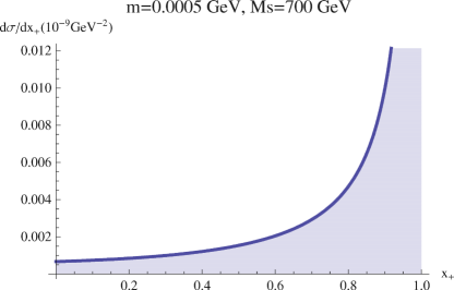
a       b c       d e       f

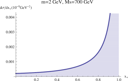
Fig. 6: The distribution of the differencial cross section on the positron energy fraction.

In the case of the interacting Majorana particles we have two essential limits for the differential cross-section (68). We have shown the cross-section dependence on masses in Fig.6(a-d). Here the filled region denotes the sum of the cross-sections in both limits $\frac{\mbox{d}\sigma_{M}}{\mbox{d}x_{+}}(\mu^{2}\ll 1)+\frac{\mbox{d}\sigma_{M}}{\mbox{d}x_{+}}(a\gg 2)$ and dashed line is the contribution of the $\frac{\mbox{d}\sigma_{M}}{\mbox{d}x_{+}}(\mu^{2}\ll 1)$ only. In other words we have shown the contribution of the term which is not proportional to the Born cross-section (finite in the zero lepton mass limit) or deviation from the Drell-Yan form of the spectrum. From the mathematical point of view we have a seesaw between $m^{2}\ln m^{2}$ and $1/a^{2}$ terms. As one can see:
– In the case of the electron mass (Fig.6a) the Born cross-section becomes negligible and the first corrections exceeds the Born level of the perturbation series. The effect is going to be maximal when the intermediate particle is light ($a\sim$2). This effect are interesting in the light of the anomalous positron flow in the Cosmic Rays bergstrom .
– If one takes muon as a lepton and the intermediate particle mass still large enough (Fig.6b) than both limits are significant and the Drell-Yan form of the spectrum is still broken.
—However, when one takes tau-lepton (Fig.6c) than still the small (in comparison with the other masses in the problem) lepton mass gives the full answer for the cross-section. The Drell-Yan form of the spectrum is restored with such parameters, so the radiative corrections are negligible. But if the intermediate particle is rather light than effect of the tau-lepton is not so crucial (Fig.6d). Thus we have shown than one should not ignore the ”small” lepton mass in the set of cases.

We show the differential cross-section for the Dirac incoming particles in Fig.6(e,f) for the comparison.

2) The cross-section averaged over both electron and positron spectra for the Dirac:

$$\sigma_{D}=\sigma_{D}^{B}(1+\frac{\alpha}{\pi}K_{D}(a))$$ (70)

and the Majorana incoming particles:

$$\sigma_{M}=\left\{\begin{array}[]{lr}\frac{\alpha|g_{L}|^{4}}{2^{7}\pi^{2}vaM^{2}}\Pi_{M},&\ \mu^{2}\ll 1\\ \sigma_{M}^{B}(1+\frac{\alpha}{\pi}K_{M}(a)),&a\gg 2,\end{array}\right.б$$ (71)

with

$$\Pi_{M}=\left(4a-1-\frac{a((11-4a)a-6)}{2a-2}\ln\left[\frac{a-2}{a}\right]\right.\\ +\left.a^{2}\left(\frac{\pi^{2}}{6}-\ln^{2}\left[\frac{a}{2a-2}\right]-2\mathcal{L}i_{2}\left[\frac{a}{2a-2}\right]\right)\right).$$

We note that K-factor is logarithmically divergent in the limit of $a\to 2$, i.e.

$$K_{i}(a)=-\frac{1}{2}\ln^{2}|a-2|+O(\ln|a-2|).$$ (72)

Remember that $a=1+\frac{M_{s}^{2}}{M^{2}}$, where $M_{S}$ and $M$ are masses of the intermediate and incoming particles, respectively. And one can obtain that K-factor blows up and exceeds another terms when

$$\mu^{2}\ln^{2}|a-2|\approx 1\quad\mbox{in other words}$$

$$\Delta M=\frac{M_{S}^{2}-M^{2}}{M^{2}}\approx e^{-\mu}$$ (73)

In this regime our result is not applicable. But physically it is almost not possible to reach it.

3) Now we should remember about full interaction Lagrangian in the eq.(1). Performing all previous calculations with respect to $g_{L}$ and $g_{R}$ terms one can get that $|g_{L}|^{4}\to(|g_{L}|^{2}+|g_{R}|^{2})^{2}$ for the Born cross-sections:

$$\sigma_{M}^{B}=\frac{(|g_{L}|^{2}+|g_{R}|^{2})^{2}m^{2}}{2^{6}\pi va^{2}M^{4}},\quad\sigma_{D}^{B}=\frac{(|g_{L}|^{2}+|g_{R}|^{2})^{2}}{2^{6}\pi va^{2}M^{2}},\quad$$

with conservation of the renormalization group structures of equations (71) and (70). Because of $g_{L}^{2}g_{R}^{2}$ terms proportional to $m^{2}$ for the Majorana case, eq.(38) and its sequences take the form:

$$F_{0}=\frac{\alpha(|g_{L}|^{4}+|g_{R}|^{4})(1-x)}{2^{4}\pi^{2}v\tau_{+}^{2}\tau_{-}^{2}M^{2}}\left[(1-x_{+})^{2}+(1-x_{-})^{2}\right].$$ (74)

K-factor is slightly changed.
4) Being integrated over the lepton energy fractions all mass singularities disappears, which is in the agreement with the Kinoshita-Lee-Nauenberg theorem KNL .

Above we had considered only t-channel Feynman amplitudes. Taking into account the s-channel diagrams with intermediate state of heavy vector neutral bosons the additional terms of order $m^{2}/M^{2}$ for the case of Dirac particles will appear. These terms will not change the results given above. For the case of Majorana particles it results in some modification of the Born cross-section still proportional to the squared lepton mass.

VII Appendix

Properties of Majorana spinors

We put here the necessary relations for the Majorana spinors CHUNG :

$$\psi^{c}=C\bar{\psi}^{T};C^{+}=C^{-1};C^{T}=-C;C^{-1}\gamma^{\mu}C=-(\gamma^{\mu})^{T};$$

$$u(k,s)=C\bar{v}^{T}(k,s);v(k,s)=C\bar{u}^{T}(k,s).$$ (75)

Bilinear combinations of Majorana spinors:

$$\sum_{s}u(p,s)\bar{u}(p,s)=\hat{p}+m;$$

$$\sum_{s}v(p,s)\bar{v}(p,s)=\hat{p}-m.$$ (76)

$$\sum_{s}u(p,s)v^{T}(p,s)=-(\hat{p}+m)C;$$

$$\sum_{s}v(p,s)u^{T}(p,s)=-(\hat{p}-m)C;$$

$$\sum_{s}\bar{u}^{T}(p,s)\bar{v}(p,s)=C^{+}(\hat{p}-m);$$

$$\sum_{s}\bar{v}^{T}(p,s)\bar{u}(p,s)=C^{+}(\hat{p}+m).$$ (77)

K-factors

Let us write down all mentioned K-factors here:
1) From calculation of the hard photon contribution we have:

$$\Phi_{M}(x_{+},x_{-}) = \frac{4[a^{2}-2ax+2(1-x_{+})(1-x_{-})][a(1+(1-x)^{2})-4x(1-x)]}{\tau_{+}^{2}\tau_{-}^{2}(2x-a)},$$ (78)

$$\Phi_{D}(x_{+},x_{-}) = \frac{1}{\tau_{+}^{2}\tau_{-}^{2}}(-a^{4}+2a^{3}(x+2)+8ax(2+x(x-2))$$

$$8(2+x(x-2))(1-x_{+})(1-x_{-})-2a^{2}(4+x^{3}+x(x_{+}+x_{-}-2x_{+}x_{-}))),$$

$$x=2-x_{+}-x_{-}.$$

2)From double differential distribution eq.(51):

$$K_{i}^{h}(x_{+},x_{-})=\frac{1}{2}[\delta(1-x_{+})(1-x_{-}+\frac{1+x_{-}^{2}}{1-x_{-}}\ln\frac{x_{-}^{2}}{1-x_{-}})+$$

$$\delta(1-x_{-})(1-x_{+}+\frac{1+x_{+}^{2}}{1-x_{+}}\ln\frac{x_{+}^{2}}{1-x_{+}})]+\Phi_{i}(x_{+},x_{-}),$$ (80)

3)From positron eq.(61):

$$K_{i}(x_{+}) = \frac{\pi^{2}}{3}-\frac{3}{4}+\frac{1}{2}[1-x_{+}+\frac{1+x_{+}^{2}}{1-x_{+}}\ln\frac{x_{+}^{2}}{1-x_{+}}]+$$ (81)

$$+ \int\limits_{1-x_{+}}^{1}\Phi_{i}(x_{+},x_{-})dx_{-}$$

and photon (eq.(62)) energy distributions

$$K^{\gamma}_{i}(x) = \frac{\pi^{2}}{3}-\frac{3}{4}+x+\frac{1+(1-x)^{2}}{x}\ln(1-x)+\int\limits_{1-x}^{1}\Phi_{i}(2-x-x_{-},x_{-})dx_{-}.$$ (82)

K-factors are small enough to be absent because they are proportional to the lepton mass and do not have any enhancement factors.

References

- (1) Marco Taoso, Gianfranco Bertone, Antonio Masiero, arXiv:0711.4996.
-
(2)
Hunter, S.D. et al. 1997, ApJ, 481, 205;
PAMELA collaboration, arXiv:0810.4995v1;…. - (3) L. Bergstrom, T. Bringmann and J. Edsjo astro-ph 0808.3725v3, Nov 2008.
-
(4)
A.V. Gladyshev, D.I. Kazakov, hep-ph/0606288,
Masaaki Kuroda,hep-ph/9902340v3. - (5) D. J. H. Chung et al., Phys. Rep. 407 (2005),p1-203.
- (6) H.K. Dreiner, H.E. Haber, S.P. Martin, arXiv:0812.1594.
- (7) H. Goldberg, Phys.Rev.Lett.50:1419,1983.
- (8) E. A. Kuraev and V. S. Fadin, Sov. J. Nucl. Phys. 41, 1985, 466, Yad. Fiz. 41,1985,733.
-
(9)
Akhiezer A. I. and Berestetsky V. B. Quantum Electrodynamics, Moscow, 1981,
M.E. Peskin, D.V. Schroeder, An introduction to Guantum Field Theory, Addison-Wesley, 1995. -
(10)
T. Kinoshita,
J. Mod. Phys., 3, 650,(1962),
T. D. Lee and M. Nauenberg, Phys. Rev. 133, B 1549 (1964).