Stability and chaotic behaviors of Bose-Einstein condensates in optical lattices with two- and three-body interactions

Abstract

The stability and chaotic behaviors of Bose-Einstein condensates with two- and three-atom interactions in optical lattices are discussed with analytical and numerical methods. It is found that the steady-state relative population appears tuning-fork bifurcation when the system parameters are changed to certain critical values. In particular, the existence of three-body interaction not only transforms the bifurcation point of the system but also affects greatly on the macroscopic quantum self-trapping behaviors of the system associated with the critically stable steady-state solution. In addition, we also investigated the influence of the initial conditions, three-body interaction and the energy bias on the macroscopic quantum self-trapping. Finally, by applying the periodic modulation on the energy bias, we find that the relative population oscillation exhibits a process from order to chaos, via a series of period-doubling bifurcations.

I Introduction

In Recent years, Bose-Einstein condensates (BECs) in optical lattices have attracted enormous attention both experimentally and theoretically ce1 ; ce2 . This is mainly because the lattice parameters and interaction strength can be manipulated using a modern experimental technique. Making use of this, researchers have discovered many long-predicted phenomena, for example non-linear Landau-Zener tunneling, energetic and dynamical instability and the strongly inhibited transport of one-dimensional BEC in optical lattices ce3 ; ce4 ; ce5 ; ce6 ; ce7 ; ce8 ; ce9 ; ce10 . More attracting phenomena, namely, self-trapping, was recently observed experimentally in this system ce11 . In such an experiment, a BEC cloud with repulsive interaction initially loaded in optical lattices was self-trapped. Many theoretical analysis was also presented about self-trapping ce12 ; ce13 ; ce14 ; ce15 . It is well know the macroscopic quantum self-trapping (MQST) means self-maintained population imbalance with non-zero average value of the fractional population imbalance which was detailed discussed ce16 ; ce17 . Marino et. al. considered that the damping decays all different oscillations to the zero-phase mode ce18 . Besides, macroscopic quantum fluctuations have also been discussed by taking advantage of second-quantization approaches ce19 . However, when the trapping potential is time dependent and the damping and finite-temperature effect can not be neglected, chaos emerges. Abdullaev and Kraenkel studied the nonlinear resonances and chaotic oscillation of the fractional imbalance between two coupled BEC’s in a double-well trap with a time-dependent tunneling amplitude for different damping ce20 . When the asymmetry of the trap potential is time-dependent and its amplitude is so small that can be took as a perturbation, Lee et al. studied the chaotic and frequency-locked atomic population oscillation between two coupled BECs with a weak damping, and discovered that the system comes to an stationary frequency-locked atomic population oscillations from transient chaos ce21 .

It is important to note that theoretical studies of stability are mainly focused on the effect of two-body interactions. It is clear that in low temperature and density, where interatomic distance is much greater than the distance scale of atom-atom interactions, two-body s-wave scattering should be important and three-body interactions can be neglected. But, if the atom density is higher, for example, in the case of BEC in optical lattices, three-body interactions will play an important role ce22 . As reported in Ref. ce23 , even for a small strength of the three-body force, the region of stability for the condensate can be extended considerably.

Therefore, the purpose of this paper is to investigate the steady-state solution of BEC in an one-dimensional periodic optical lattice when both the two-body and three-body interactions are taken into account. By using the mean-field approximation and linear stability theorem, one interesting result is found that the tuning-fork bifurcation of steady-state relative population appears when the system parameters are changed to certain critical values. The existence of three-body interaction not only transforms the bifurcation point of the system but also affects greatly on the self-trapping behaviors of the system associated with the critically stable steady-state solutions. Additionally, we also study the effects of the initial conditions, three-body interaction and the energy bias on the MQST. Besides, we discuss the chaos behaviors of the system by applying the periodic modulation on the energy bias. The result shows the relative population oscillation can undergo a process from order to chaos, via a series of period-doubling bifurcations.

This paper is organized as follows. In Sec. II, we introduce the mean-field description of BEC in optical lattices with two- and three-atom interactions. In Sec. III, with linear stability theorem, we analysis the stability of steady-state solutions. Then the influences of three-body interaction on the macroscopic quantum self-trapping of the system are displayed In Sec. IV. In Sec. V, by applying the periodic modulation in the energy bias, we discuss chaotic behaviors of the system using the numerical simulation method. In the last section, summary and conclusion of our work are presented.

II Mean-field description of BEC in optical lattices with two- and three-atom interactions

We focus our attention on a BEC with both two- and three-body interactions is subjected to one dimensional (1D) optical lattices where the motion in the perpendicular directions is confined. In the mean-field approximation , the dynamics of BEC can be modeled by the 1D Gross-Pitaevskii (GP) equation in the comoving frame of the lattice ce3 ; ce6 ; ce24 ; ce25 ,

$$i\hbar\frac{\partial\Phi}{\partial t}=-\frac{1}{2m}\left(\hbar\frac{\partial}{\partial t}-ima_{l}t\right)^{2}\Phi+\upsilon_{0}\cos(2K_{l}x)\Phi+\frac{2\hbar^{2}a_{s}}{a_{\bot}^{2}m}|\Phi|^{2}\Phi+\frac{g_{2}}{3\pi^{2}a_{\bot}^{4}}|\Phi|^{4}\Phi,$$ (1)

where $\Phi$ is the wave function of the condensate, $m$ is the mass of atoms, $a_{s}$ is the two-body s-wave scattering length, $\upsilon_{0}$ is the strength of the periodic potential, $K_{l}$ is the wave number of the laser light which is used to generate the optical lattice, $ma_{l}$ stands for either the inertial force in the comoving frame of an accelerating lattice or the gravity force, $a_{\bot}=\sqrt{\hbar/(m\omega_{\bot})}$, where $\omega_{\bot}$ is the radial frequencies of the anisotropic harmonic trap, $g_{2}|\Phi|^{4}\Phi/(3\pi^{2}a_{\bot}^{4})$ is three-body interactions related to the GP equation. Among Eq. (1), all the variables can be rescaled to be dimensionless by the following system’s basic parameter $x\sim 2K_{l}x,\Phi\sim\frac{\Phi}{\sqrt{2K_{l}N}},t\sim\frac{4\hbar}{m}K_{l}^{2}t$. we obtain the normalized 1D-GP equation in optical lattices with cubic and quintic nonlinearities,

$$i\frac{\partial\Phi}{\partial t}=-{{1}\over{2}}\left(\frac{\partial}{\partial t}-i\alpha t\right)^{2}\Phi+\upsilon\cos(x)\Phi+c|\Phi|^{2}\Phi+\lambda|\Phi|^{4}\Phi,$$ (2)

where $\upsilon=\frac{m\upsilon_{0}}{4\hbar^{2}K_{l}^{2}},\alpha=\frac{m^{2}}{8\hbar^{2}K_{l}^{3}}a_{l},c=\frac{Na_{s}}{K_{l}a\bot^{2}}$ is the effective two-body interaction, $N$ is the total numbers of atoms, $\lambda=\frac{mg_{2}N^{2}}{3\pi^{2}\hbar^{2}a_{\bot}^{4}}$ is the effective interaction among three atoms, here the three-body interaction is expected to be positive with a value of $0<\lambda<1$.

In the neighborhood of the Brillouin Zone edge $k=1/2$, the wave function can be approximated by ce3

$$\Phi(x,t)=a(t)e^{ikx}+b(t)e^{i(k-1)x},$$ (3)

where $a(t)$, $b(t)$ are the probability amplitudes of atoms in each of the two wells respectively and $|a|^{2}+|b|^{2}=1$. By inserting such wave functions into Eq. (2) and performing some spatial integrals, we obtain the dynamical equations with two- and three-body interactions.

$$i\frac{\partial a}{\partial t} = \frac{\gamma}{2}a+\frac{c}{2}\left(|b|^{2}-|a|^{2}\right)a+\lambda\left(1+2|a|^{2}|b|^{2}+2|b|^{2}\right)a+\frac{\upsilon}{2}b,$$ (4)

$$i\frac{\partial b}{\partial t} = -\frac{\gamma}{2}b-\frac{c}{2}\left(|b|^{2}-|a|^{2}\right)b+\lambda\left(1+2|a|^{2}|b|^{2}+2|b|^{2}\right)b+\frac{\upsilon}{2}a.$$ (5)

Here, the level bias $\gamma(t)=\alpha t$, and $\alpha$ is the sweeping rate, $c$ and $\lambda$ represent the nonlinear parameters, $\upsilon$ is the coupling constant between the two condensates. We introduce the relative population variance

$$s=|b|^{2}-|a|^{2},$$ (6)

with the parameters $a=|a|e^{i}\theta_{a}$, $b=|b|e^{i}\theta_{b}$,

$$\theta=\theta_{b}-\theta_{a}.$$ (7)

Combining Eqs. (4-7), one yields the equations of the relative population and relative phase,

$$\dot{s} = -\upsilon\sqrt{1-s^{2}}\sin\theta,$$ (8)

$$\dot{\theta} = \gamma+(c+2\lambda)s+\frac{\upsilon s}{\sqrt{1-s^{2}}}\cos\theta.$$ (9)

$\dot{s}$ and $\dot{\theta}$ denote the time derivative of the relative population and the relative phase. If we regard $s$ and $\theta$ as the canonically conjugate variables Eqs. (8) and (9), become a pair of Hamilton’s canonical equations with the conserved effective Hamiltonian

$$H=\gamma s+\frac{1}{2}(c+2\lambda)s^{2}+\upsilon\sqrt{1-s^{2}}\cos\theta.$$ (10)

In the following section, we will discuss the stability of steady-state in the symmetric condition ($\gamma=0$) with linear stability theorem.

III Stability analysis of the steady-state solutions

In Sec. II, we have given the dynamical equations of the system with three-body interaction. In this section, we will discuss the stability of steady-state in the symmetric condition. Generally, there are two ways to study the stability of nonlinear system, the linear stability theorem and the Lyapunov direct method. We will investigate the stability of the system with the first method.

The steady-state solution of this system can be obtained by setting Eqs. (8) and (9) to zero. The forms of steady-state solutions are very complicated when the level bias $\gamma\neq 0$. For simplicity, we set $\gamma=0$, leading to

$$\dot{s} = f_{1}(s,\theta)=-\upsilon\sqrt{1-s^{2}}\sin\theta,$$ (11)

$$\dot{\theta} = f_{2}(s,\theta)=(c+2\lambda)s+\frac{\upsilon s}{\sqrt{1-s^{2}}}\cos\theta.$$ (12)

and the conserved energy

$$H=\frac{1}{2}(c+2\lambda)s^{2}+\upsilon\sqrt{1-s^{2}}\cos\theta.$$ (14)

Taking $\dot{s}=0$, $\dot{\theta}=0$, we get

$$-\upsilon\sqrt{1-s^{2}}\sin\theta = 0,$$ (15)

$$(c+2\lambda)s+\frac{\upsilon s}{\sqrt{1-s^{2}}}\cos\theta = 0.$$ (16)

The steady-state solutions obeyed Eqs. (14) and (15) regard as

$$\theta_{1} = 2n\pi,\quad s_{1}=0\quad\mathrm{for}\quad H=-\upsilon,$$ (17)

$$\theta_{2} = (2n+1)\pi,\quad s_{2}=0\quad\mathrm{for}\quad H=\upsilon,$$ (18)

$$\theta_{3,4}=(2n+1)\pi,\quad s_{3,4}=\pm\sqrt{1-(\frac{\upsilon}{c+2\lambda})^{2}}\quad\mathrm{for}\quad H=\frac{(c+2\lambda)^{2}+\upsilon^{2}}{2(c+2\lambda)^{2}}.$$ (19)

According to the linear stability theorem, we look for the perturbed solutions which are near the steady-state solutions,

$$s(t)=s_{i}(t)+\varepsilon_{1}(t),\qquad\theta(t)=\theta_{i}(t)+\varepsilon_{2}(t)$$ (20)

where $s_{i}(t)$, $\theta_{i}(t)$ for $i=1,2,3,4$ signify the steady-state solutions, $|\varepsilon_{1}(t)|\ll|s_{i}(t)|$ and $|\varepsilon_{2}(t)|\ll|\theta_{i}(t)|$ which is relate to the first-order perturbed. Inserting the above expression into Eqs. (11) and (12), we can obtain the linear equations near to the steady-states of the nonlinear equations as

$$\dot{\varepsilon_{1}}=\left(\frac{\partial f_{1}}{\partial s}\right)_{1}\varepsilon_{1}+\left(\frac{\partial f_{1}}{\partial\theta}\right)_{1}\varepsilon_{2}\qquad namely\qquad\dot{\varepsilon_{1}}=a_{11}\varepsilon_{1}+a_{12}\varepsilon_{2}$$ (21)

$$\dot{\varepsilon_{2}}=\left(\frac{\partial f_{2}}{\partial s}\right)_{2}\varepsilon_{1}+\left(\frac{\partial f_{2}}{\partial\theta}\right)_{2}\varepsilon_{2}\qquad namely\qquad\dot{\varepsilon_{2}}=a_{21}\varepsilon_{1}+a_{22}\varepsilon_{2}$$ (22)

Now, we make use of the above expression to investigate the stability of the steady-states of Eqs. (16-18).

(1)For $\theta_{1}=2n\pi,s_{1}=0,H=-\upsilon$, we can calculate the matrix elements $a_{11}=0$, $a_{12}=-\upsilon$, $a_{21}=(c+2\lambda)+\upsilon$, $a_{22}=0$. So, the coefficient matrix of the linearized equations (20) and (21) becomes $A_{1}=\left[\begin{array}[]{cc}{0}&{-\upsilon}\\ {c+2\lambda+\upsilon}&{0}\\ \end{array}\right]$ such that the characteristic equation writes $\det(A_{1}-\lambda I)=\left[\begin{array}[]{cc}{0-\lambda}&{-\upsilon}\\ {c+2\lambda+\upsilon}&{0-\lambda}\\ \end{array}\right]=0$, which reveals that $\lambda^{2}+\upsilon(c+2\lambda+\upsilon)=0$. We solve the equation to get the two eigenvalues of the matrix A as $\lambda_{1}=\sqrt{-\upsilon(c+2\lambda+\upsilon)},\lambda_{2}=-\sqrt{-\upsilon(c+2\lambda+\upsilon)}$. In response to the forms of the eigenvalues, there exist two cases for the stabilities:

(a) $\upsilon(c+2\lambda+\upsilon)\geq 0$, that is

$$\upsilon>0\quad and\quad(c+2\lambda)\geq-\upsilon$$ (23)

$$\upsilon<0\quad and\quad(c+2\lambda)\leq-\upsilon$$ (24)

so the two eigenvalues are both pure imaginary numbers. Thus, the stability of the steady-state solutions $(\theta_{1},s_{1})$ corresponds to a critical case ce26 and the dynamical bifurcations between the unstable and stable steady-states will appear when the parameters with two- and three-body interactions are changed.

(b) $\upsilon(c+2\lambda+\upsilon)<0$, namely

$$\upsilon>0\quad and\quad(c+2\lambda)<-\upsilon$$ (25)

$$\upsilon<0\quad and\quad(c+2\lambda)>-\upsilon$$ (26)

so the two eigenvalues are real number. It means that $\varepsilon_{1}$ and $\varepsilon_{2}$ tend to infinity with the increase of time, and the steady-state solutions $(\theta_{1},s_{1})$ are unstable.

(2)For $\theta_{2}=(2n+1)\pi$, $s_{2}=0$, $H=\upsilon$, the matrix elements write as $a_{11}=0,a_{12}=-\upsilon,a_{21}=(c+2\lambda)-\upsilon,a_{22}=0$. The corresponding eigenvalues of the matrix $A_{2}$ become $\lambda_{1}=\sqrt{-\upsilon(\upsilon-(c+2\lambda))},\lambda_{2}=-\sqrt{-\upsilon(\upsilon-(c+2\lambda))}$. Similarly, there are two cases of the stabilities:

(a) $\upsilon(\upsilon-(c+2\lambda))>0$, that is

$$(c+2\lambda)>0\quad \mathrm{and}\quad\upsilon>(c+2\lambda)$$ (27)

$$(c+2\lambda)<0\quad \mathrm{and}\quad\upsilon>0.$$ (28)

so the two eigenvalues are both pure imaginary numbers. And the stability of the steady-state solutions $(\theta_{2},s_{2})$ of the nonlinear equations are reviewed as critical and the dynamical bifurcations will occur.

(b) $\upsilon(\upsilon-(c+2\lambda))\leq 0$, that is

$$\upsilon>0\quad \mathrm{and} \quad(c+2\lambda)\geq\upsilon$$ (29)

$$(c+2\lambda)<\upsilon\quad \mathrm{and} \quad\upsilon<0$$ (30)

so the two eigenvalues are positive or negative real number, respectively. $\varepsilon_{1}$, $\varepsilon_{2}$ tend to infinity as increasing the time to infinity, and the steady-state solutions $(\theta_{2},s_{2})$ are losing their stability.

(3)For $\theta_{3,4}=(2n+1)\pi,s_{3,4}=\pm\sqrt{1-(\frac{\upsilon}{c+2\lambda})^{2}},H=\frac{(c+2\lambda)^{2}+\upsilon^{2}}{2(c+2\lambda)^{2}}$, the matrix elements read $a_{11}=0$, $a_{12}=\upsilon^{2}/(c+2\lambda)$, $a_{21}=(c+2\lambda)-(c+2\lambda)^{3}/\upsilon^{2}$, $a_{22}=0$, and the eigenvalues $\lambda_{1}=\sqrt{\upsilon^{2}-(c+2\lambda)^{2})}$, $\lambda_{2}=-\sqrt{\upsilon^{2}-(c+2\lambda)^{2})}$. In Eq. (18) the population $s_{3,4}$ are both real quantities which implies

$$(c+2\lambda)^{2}>\upsilon^{2}$$ (31)

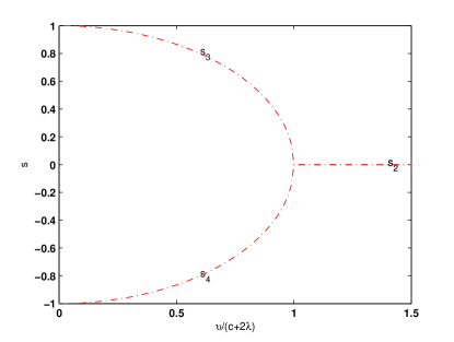
Figure 1: Plots of the tuning-fork bifurcation from Eqs. (17) and (18), where $s_{2},s_{3},s_{4}$ are the steady-state solutions and the bifurcation point is $\frac{\upsilon}{c+2\lambda}=1$

Therefore, the two eigenvalues are pure imaginary numbers. The stability of the steady-state solutions$(\theta_{3,4},s_{3,4})$ of the nonlinear equations are regarded as critical and the dynamical bifurcations will emerge at the bifurcation point $(c+2\lambda)=\upsilon$, $s=0$. Obviously, the existence of three-body interaction can change the bifurcation point of the system. It plays a important role for stability analysis of the system, as shown in Fig. 1. For $\frac{\upsilon}{c+2\lambda}>1$, the system is in the critically stable steady-state ($\theta_{2},s_{2}$), and for $\frac{\upsilon}{c+2\lambda}<1$, ($\theta_{2},s_{2}$) is unstable and the two steady-state solutions ($\theta_{3,4},s_{3,4}$) are critically stable. This is a typical tuning-fork bifurcation, and the bifurcation point is $\frac{\upsilon}{c+2\lambda}=1$

According to the above analysis, we conclude that three steady-state solutions possess different stability for different parameter regions. And it is very interesting to arrive at the critically stable steady-state solution in experiment which relate to the stable stationary MQST ce26 . In the following section, we will illustrate the MQST of the non-stationary states in detail by two different methods.

IV The macroscopic quantum self-trapping of BEC with two- and three-atom interactions

In this section, we investigate the macroscopic quantum self-trapping by plotting the phase trajectories and the time evolution of the relative population of the system.

IV.1 The phase trajectories diagram

The macroscopic quantum self-trapping refers to the phase space trajectories whose the relative population is not equal zero. This can be well understood from the analysis Eqs. (8)-(10), corresponding to the critically stable steady-state solutions discussed in sec.II. Three kinds of cases occur with different three-body interaction parameters, as shown in Fig.2.

(1) In the case of $\upsilon=0.2,c=0.1,0<\lambda<0.05$ in the phase space , there are two stable points $P_{1},P_{2}$ at $s=0,\theta=\pi$ and $s=0,\theta=0$ respectively [Fig. 2(a)], from the circumstance described by Eqs. (22) and (26). Obviously, for the stable points $P_{1}$, $P_{2}$, the atoms distributions are equal in the two adjacent wells, the relative population of the trajectories around them is equal to $0$. It means that atoms oscillate between two adjacent wells and the macroscopic quantum self-trapping phenomenon does not emerge in this case.

(2) When parameter is set to $\upsilon=0.2$, $c=0.1$, $0.05\leq\lambda<0.15$, two more fixed points emerge in the line $\theta=\pi$ marked by $P_{3}$, $P_{4}$. Among them, $P_{1}$, $P_{3}$ are steady which is corresponding to condition of Eq. (30). They are located in $s=\pm\sqrt{1-(\frac{\upsilon}{c+2\lambda})^{2}}$, hence, $P_{4}$ is unstable point which lies in $s=0$ and corresponds to condition of Eq.(26). As seen from Fig. 2(b), for the stable points $P_{1},P_{3}$, the atoms distributions are not equilibrium between two adjacent wells, and the relative population of the trajectories around them is not equal to $0$. It indicates that atoms are self-trapped in one well. We take it as oscillating-phase-type because the relative population $s$ and the relative phase $\theta$ oscillate around the fixed points.

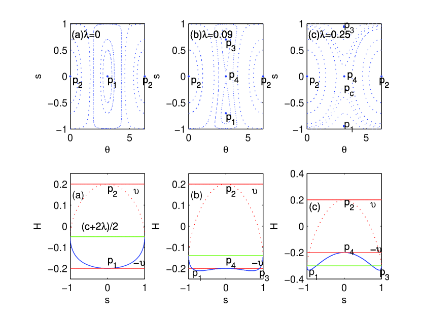
Figure 2: Trajectories on the phase space of the system with three-body interaction varying from $\lambda=0$ to $\lambda=0.25$(the first row). Corresponding to in the second row we plot the energy profiles for the relative phase $\theta=0$ (red dashed) and $\theta=\pi$ (blue solid)

(3) For $\upsilon=0.2,c=0.1$, $\lambda\geq 0.15$ , It emerges new trajectories , i.e.the trajectories across point $P_{c}$ [Fig. 2(c)]. Only the fixed point $P_{2}$ is stable which is relate to Eq. (22). So for these trajectories, $s$ varies with time from region of $[-1,0]$ to $[0,1]$, Apparently $\langle s\rangle\neq 0$, atoms are self-trapped in one well. We regard it as running-phase-type macroscopic quantum self-trapping, as described in Refs. ce27 ; ce28 and observed in experiment ce29 .

The above changes on the topological structure of the phase space are concerned with the change of the energy profile. When the relative phase is zero or $\pi$, energy relying on the parameter with three-body interaction and the average population $s$ can be derived from Eq. (10). Seeing Fig. 2 , the transition from case(1)to case(2) corresponds to the bifurcation of the energy profile of $\theta=\pi$: energy curve bifurcates from a single minimum to the curve of two minima. It means the system goes from the Rabi regime into the self-trapping regime through this bifurcation. The lowest order of energy profile with $\theta=0$ is $-\frac{c+2\lambda}{2}$, and the energy of the unstable point $P_{4}$ is $-\upsilon$ which is located on the maximal order of energy profile with $\theta=\pi$. The results displayed by the phase space trajectories conform to the case of steady-state solutions discussed in Sec.III. The transition from case (2) to case(3) is signified by the overlap of the two energy regions of the profile. In this condition the trajectory stared from $s=-1$, $\theta=0$ should be confined to the lower half of phase plane, corresponding to the running-phase-type macroscopic quantum self-trapping.

Connecting the analysis of the steady-state solutions to the above analysis on the energy profile, it concludes that stable behaviors of the system change constantly with the increase of $\lambda$ and we obtain a general criterion for the macroscopic quantum self-trapping trajectories, namely, $H(s,\theta)<-\upsilon$. It plays a critical role to find the transition parameters of macroscopic quantum self-tapping.

IV.2 Numerical simulations of the MQST

Now, we focus on the dynamic behavior which dominated by Eq. (8) and (9) without the time-dependent system parameters. We study the effect parameters of the system on the MQST with numerical method starting form Eq. (8) and (9).

Figure 3: The time evolution of the relative population from Eqs.(8) and (9) with initial conditions $s(0)=0$, $\theta_{0}=\pi/2$ and parameter: (a) $c=0.1$, $\lambda=0.45$, $v=0.2$, and $\gamma=0$; (b) $c=0.1$, $\lambda=0.95$, $v=0.2$, and $\gamma=0$; (c) $c=0.1$, $\lambda=0.45$, $v=0.8$, and $\gamma=0$; (d) $c=0.1$, $\lambda=0.45$, $v=0.2$, and $\gamma=0.5$; (e) $c=0.1$, $\lambda=0.95$, $v=0.2$, and $\gamma=0.5$; (f) $c=0.1$, $\lambda=0.45$, $v=0.8$, and $\gamma=0.5$;

Figure 4: the time evolution of the relative population from Eqs. (8) and (9). (a) initial conditions $s(0)=0.8$, $\theta_{0}=\pi$ (b) initial conditions $s(0)=0.8$, $\theta_{0}=\pi/2$, and the other parameters $c=0.1$, $\lambda=0.45$, $v=0.2$, and $\gamma=0$.

Choosing initial condition $s(0)=0$, $\theta(0)=\pi/2$, the time evolutions of the relative population Fig. (3a)-(3d) show some very absorbing features. In Fig. 3(a), the oscillations are regular and the average the relative population $\bar{s}$ is zero for symmetric well case ($\gamma=0$) with a special parameter, but the corresponding MQST does not appear. If we increase $\lambda$ from 0.45 to 0.95 in Fig. 3(b), the MQST does not still appear, but the oscillating period becomes short. Similarly, rising $\upsilon$ , we obtain the same result as shown in Fig. 3(c).

Here, we study impacting asymmetric well case ($\gamma\neq 0$) on the MQST. when we enhance the level bias to $\gamma=0.5$ the average the relative population is changed to $-0.41$ in Fig.3(d). Correspondingly, the oscillating period of $s$ is longer and the MQST emerges. Note that parameter $c$, $\lambda$ and $\upsilon$ impact greatly on the MQST which are plotted in Fig. 3(e) and (f). In fig. 3(e), when $\lambda$ is from $0.45$ to $0.95$, the MQST is suppressed with shorter oscillating period. Similarly, with increasing $\upsilon$, the average relative population are changed to $-0.21$ and the oscillating period becomes shorter again, as seen in Fig. 3(f). Thus, the influence of parameter $c$ ,$\lambda$ ,$\upsilon$ and $\gamma$ on the MQST of the system is very dramatic. In the case of $\gamma=0$, fixing the other parameters and changing the initial condition from $s(0)=0,\theta(0)=\pi/2$ of Fig.3 to $s(0)=0.8,\theta(0)=\frac{\pi}{2}$ and $s(0)=0.8,\theta(0)=\pi$, we observe that the MQST always emerges with varying $s(0),\theta(0)$. The oscillating period is decreased comparing to Fig.3(a)and Fig. 3(d), but the $\bar{s}$ is increased to $-0.86,-0.72$ as shown in Fig. 4.

According to the above analysis, we can draw conclusion that when the initial conditions $s(0)=0$, $\theta(0)=\pi/2$ are read, the parameter $c$, $\lambda$, $\upsilon$ can impact on the MQST for asymmetric well case($\gamma\neq 0$). In addition, in the symmetric case, the MQST does not appear and those parameters only affect the oscillating period of the system. Besides, the initial conditions can impact the MQST for anyone parameter set.

V Numerical simulation of chaos by applying periodic modulation on the lever bias

As a whole, the elementary features of chaos is that the dynamic behaviors are unpredictable for a deterministic system. It is very sensitive for the initial conditions and parameters of the system. So, according to these characteristics, we can adjust the parameters to make the system get into or get out of the chaos, in other words, we can control the regime appearing chaos. In this section We discuss the chaotic behaviors of the system by numerical method.

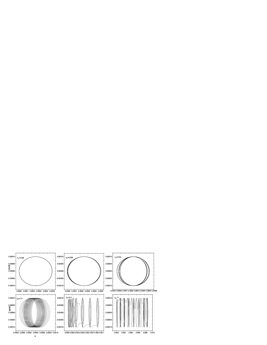
Figure 5: Dynamical phase orbits of the dimensionless variables ($s,ds/dt$) from Eqs. (31) and (32) with parameters $\upsilon=0.001$, $c=0.1$, $\lambda=0.45$, $\omega=0.1$, $s(0)=0$, $\theta_{0}=\pi$, and (a) $A_{1}=0.002$, (b) $A_{1}=0.009$, (c) $A_{1}=0.04$, (d) $A_{1}=0.12$, (e) $A_{1}=0.3$, (f)=$A_{1}=1$. Here, $A_{1}$ denotes the amplitude of the time-dependent relative energy.

If we apply periodic modulation on the lever bias $\gamma=A_{0}+A_{1}sin(\omega t)$, the chaos will appear in a special region, where $A_{0},A_{1}$ stand for initial phase and amplitude respectively. Inserting this into Eqs. (8)and (9), one derives the below dynamic equation.

$$\dot{s} = -\upsilon\sqrt{1-s^{2}}\sin\theta$$ (32)

$$\dot{\theta} = A_{0}+A_{1}\sin(\omega t)+(c+2\lambda)s+\frac{\upsilon s}{\sqrt{1-s^{2}}}\cos\theta$$ (33)

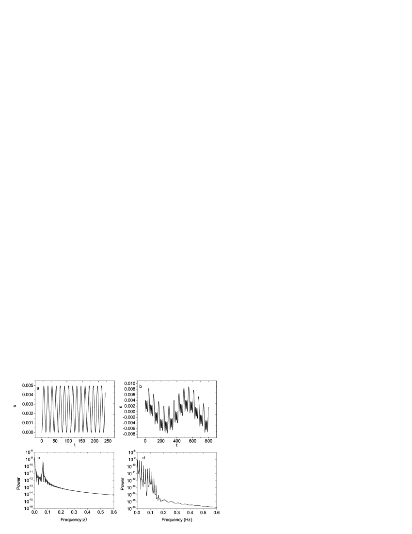
Figure 6: (a) and (b): The time evolution of the relative population of the relative population from Eqs. (31)and (32) with the parameters $\upsilon=0.001$, $A_{0}=0.4$, $c=0.1$, $\lambda=0.45$, $\omega=0.1$, $s(0)=0$, $\theta(0)=\pi$, and (a) $A_{1}=0.002$, (b) $A_{1}=0.3$ (c) and (d): The corresponding power spectrum, where the parameters in Fig. 6(c)are the same with Fig. 6(a) and the parameters in Fig. 6(d)are the same with Fig. 6(b).

Starting from Eqs. (32), It is found that the dynamics behavior of the system is periodic in some special parameters region and it will vary from order to chaos with the increase of $A_{1}$ , as shown in Fig.5. With initial conditions $s(0)=0,\theta(0)=\pi$, the phase orbit is a period-one cycle and the corresponding oscillation is a Rabi oscillation for the set of parameters with amplitude $A_{1}=0.002$, as in Fig. 5(a). In this case, we set the oscillating period of the relative population $T$. When $A_{1}=0.009$, the phase orbit becomes period-two in Fig. 5(b). It means the oscillating period of $s$ arriving at $2T$. Then the phase orbit increases from that of period-four to period-eight with increasing $A_{1}$ as shown in Fig. 5(c)and (d). Fig. 5(e) and 5(f) are plotted for $A_{1}=0.3$ and $A_{1}=1$, where the phase orbit does not show a clear periodicity which signifies the emergence of chaos.

From the above analysis, we find that the oscillating period of the relative population varies from a period-one limit-cycle to period-two to period-four and then to period-eight and finally all limit-cycles tend to infinity with $\gamma$ increasing. It exhibits a process from order to chaos, through the period-doubling bifurcations ce26 . That is to say, for a set of fixed parameter $\upsilon$, $c$, $\lambda$, $A_{0}$, $A_{1}$, $s(0)$, $\theta(0)$ and $\omega$, the first-order derivative of relative population transform from the single period to multiple period and get into chaos at last with the increase of vibration amplitude $A_{1}$.

For the aim of showing the chaotic MQST, we present the plots of the time evolution of the relative population and corresponding plots of power spectra from Eqs. (31) and (32) in Fig. 6. And the parameter of Fig.5(a) is accord with Fig. 6(a) and 6(c) where the system oscillates periodically. Making use of those parameters of Fig. 5(e), we plot Fig. 6(b)and 6(d). It shows that the power spectrum appears confusion and the average value of the relative population is less than zero, which implies the existence of the chaotic behaviors .

VI Summary and conclusion

In this paper, we study the stability and chaos of BEC with repulsive two- and three-body interactions immersed in a one-dimensional optical lattice. The stability of the steady-state solution are analyzed with the linear stability theorem. The analytical results show: (1) For $\upsilon>0$ and $c+2\lambda\geq-\upsilon$ or $\upsilon<0$ and $c+2\lambda\leq-\upsilon$, the stability of the steady-state solution($\theta_{1}=2n\pi,s_{1}=0$) is in the critical case. (2) For $c+2\lambda>0$ and $\upsilon>c+2\lambda$ or $c+2\lambda<0$ and $\upsilon>0$, the steady-state solution($\theta_{2}=(2n+1)\pi,s_{2}=0$) is the critical stability. (3) For $(c+2\lambda)_{2}>\upsilon_{2}$, the steady-state solution ($\theta_{3,4}=(2n+1)\pi,S_{3,4}=\pm\sqrt{1-(\frac{\upsilon}{c+2\lambda})^{2}}$) is also critically stable. When these relationship are not satisfied, the corresponding steady-state solution are unstable. A typical tuning-fork bifurcation of steady-state relative population appears in special parameter region. And the existence of three-body interaction can change the bifurcation point of the system, which is shown as Fig. 1. It plays a important role for stability analysis of the system.

The critically stable steady-state solution indicates the existence of the stationary MSQT. The stable behaviors of the system change constantly with the increase of $\lambda$ and get a general criteria for the self-trapping trajectories, $H<-\upsilon$. In addition, we also investigate the effects of the initial conditions, a set of parameters $c,\upsilon,\lambda,\gamma$ on MQST. It shows that $c,\upsilon,\lambda$ could affect on the MQST when $s(0)=0,\theta_{0}=\pi$ for $\gamma\neq 0$. Particularly, the initial value $s(0)=0,\theta_{0}=\pi$ or $s(0)=0,\theta_{0}=\pi/2$ can directly impact on the MQST. Finally, we discuss the chaos behaviors by applying the modulation on the energy bias ($\gamma=A_{0}+A_{1}sin\omega t$). In this case, the system will go into chaos through the period-doubling bifurcations with the increasing of $\lambda$, and the time evolution of the relative population and power spectra indicate the existence of the chaos MQST. It suggests that one can adjust the lasing detuning and intensity to change the values of the parameters in experiments. This adjustable parameters supply the possibility for controlling the instabilities of the system, MQST state and the chaotic behaviors.

- (1) J. K. Chin, D. E. Miller, Y. Liu, C. stan, W. Setiawan, C. Sanner, K. Xu, and W. Ketterle, Nature (London) 443, 961 (2006).
- (2) J. K. Xue and A. X. Zhang, Phys. Rev. Lett. 101, 180401 (2008).
- (3) B. Wu and Q. Niu, Phys. Rev. A 61, 023402 (2000).
- (4) B. Wu, R. B. Diener, and Q. Niu, Phys. Rev. A 65, 025601 (2002).
- (5) J. Liu et al., Phys. Rev. A 66, 023404 (2002).
- (6) L. M. JonaM, O. Morsh, M. Cristiani, N. Malossi, J. H. Muller, E. Couritade, M. Anderlini, and E. Arumondo, Phys. Rev. Lett. 91, 230406 (2003).
- (7) D. Diakonov et al., Phys. Rev. A 66, 013064 (2002).
- (8) Mueller E J, Phys. Rev. A 66. 063603 (2002).
- (9) L. Fallni, L. D. Sarlo, J. E. Lye, M. Modugno, R. Saer, C. Fort, and M. Inguscio, Phys. Rev. Lett. 93, 140406 (2004).
- (10) T. Koponen, J. P. Martikainen, J. Kinnunen, and P. Torma, Phys. Rev. A 973, 033620 (2006).
- (11) S. K. Adhikari and B. A. Malomed, Europhy. Lett. 79, 50003 (2007); Phys. Rev. A 76, 043626 (2007).
- (12) B. Wu and Q. Niu, New J. Phys. 5, 104 (2003).
- (13) O. Morsch and M. Oberthaler, and D. Ionut, Rev. Mod. Phys. 78, 179 (2006).
- (14) B. Liu, L. B. Fu, S. P. Yang, and J. Liu, Phys. Rev. A 75, 033601 (2007).
- (15) G. F. Wang, D. F. Ye, L. B. Fu, X. Z. Chen, and J. Liu, Phys. Rev. A 74, 033414 (2006).
- (16) A. Smerzi, S. Fantoni, S. Giovanzzi, and S. R. Shenoy, Phys. Rev. Lett. 79, 4950 (1997).
- (17) S. Raghavan, A. Smerzi, S. Fantoni, and S. R. shenoy, Phys. Rev. A 59, 620 (1999).
- (18) I. Marino, S. Fantoni, S. R. shenoy, and A. Smerzi, Phys. Rev. A 60, 487 (1999).
- (19) A. Smerzi and S. Raghavan, Phys. Rev. A 61, 063601 (2000).
- (20) F. K. Abdullaev and R. A. Kraenkel, Phys. Rev. A 62, 023613 (2000).
- (21) C. Lee, W. Hai, L. Shi, X. Zhu, and K. Gao, Phys. Rev. A 64, 053604 (2001).
- (22) T. Kohler, Phys. Rev. Lett. 89, 210404 (2002).
- (23) N. Akhmediev, M. P. Das, and A. V. Vagov, Int. J. Mod. Phys. B 13, 625 (1999).
- (24) A. X. Zhang and J. K. Xue, Phys. Rev. A 75, 013624 (2007).
- (25) Q. Niu and M. G. Raizen, Phys. Rev. Lett. 80, 3491 (1998).
- (26) B. Z. Liu and J. H. Peng, Nonlinear Dynamics (Advanced Education Publishing House, Beijing, 2004). (in Chinese)
- (27) S. Raghavan, A. Smerzi, and V. M. Kenkre, Phys. Rev. A 60, 1787 (1999).
- (28) M. Holthaus, Phys. Rev. A 64, 011601 (2001).
- (29) M. Albiez et al., Phys. Rev. Lett. 79, 4950 (1997).