Phase transition of $q$-state clock models on heptagonal lattices

Abstract

We study the $q$-state clock models on heptagonal lattices assigned on a negatively curved surface. We show that the system exhibits three classes of equilibrium phases; in between ordered and disordered phases, an intermediate phase characterized by a diverging susceptibility with no magnetic order is observed at every $q\geq 2$. The persistence of the third phase for all $q$ is in contrast with the disappearance of the counterpart phase in a planar system for small $q$, which indicates the significance of nonvanishing surface-volume ratio that is peculiar in the heptagonal lattice. Analytic arguments based on Ginzburg-Landau theory and generalized Cayley trees make clear that the two-stage transition in the present system is attributed to an energy gap of spin-wave excitations and strong boundary-spin contributions. We further demonstrate that boundary effects breaks the mean-field character in the bulk region, which establishes the consistency with results of clock models on boundary-free hyperbolic lattices.

I Introduction

The role of geometry has continued drawing attention in statistical physics. A curved surface, for example, has been a useful test ground to study ergodicity balazs , and curved nanoscale carbon structures have been expected to possess interesting elastic and magnetic properties nano . Recently, rapid development of soft material sciences also requires a precise understanding of physics on a curved surface in terms of geometric interactions kamien-hemmen . One immediate question from the statistical-physical viewpoint is how phase transitions occur on such a curved surface since they in general depend on geometrical factors. In particular, a negative Gaussian curvature yielding a saddle-like hyperbolic surface has been more commonly studied in critical phenomena than a positive one since a positive curvature tends to make a closed surface so that it is hard to extend the system size while keeping the magnitude of the curvature constant. In a negatively curved surface, the length scale grows only logarithmically with the surface area, and thus one could expect a mean-field-like critical behavior in many systems. Whereas this expectation was proven true for the bulk of the Ising spin system shima ; ueda , the $XY$ spin model has no local order at finite temperatures xy . This lack of order in the $XY$ model is attributed to the gapless spin-wave excitations that can arise from the boundary at any finite temperature $T$. This argument is based on the fact that a negatively curved surface contains a huge amount of boundary points: that is, for a negatively curved surface, the ratio of surface area to perimeter (which is the two-dimensional example of the so-called surface-volume ratio in general dimension) remain nonvanishing even in the large-system limit. Since it was pointed out that a system may have a novel behavior due to the presence of a nonvanishing boundary auriac , there have been ongoing studies to clarify this issue shima ; shima2006a ; xy ; diff ; perc ; geomxy . While the boundary effects can be sometimes excluded, for example, by using a periodic boundary condition sausset or by mathematical abstractions belo ; ueda ; gendiar ; krcmar , it is often crucial to understand how a boundary affects the physical properties since it may give the most important contribution to an observed behavior as will be explained in this work.

The complete difference between the Ising and the $XY$ models with respect to the presence or absence of the ordered phase motivates us to study the $q$-state clock model on a negatively curved surface. The $q$-state clock model is equivalent to the Ising model for $q=2$ and approaches to the $XY$ model for $q\rightarrow\infty$. Thereby one can obtain a better understanding on how the phase structure changes in between with varying $q$. In this paper, we present the following findings: first, the critical temperature $T_{c}$ is indeed proportional to the energy gap to excite the spin fluctuations. second, we report an intermediate phase with a diverging susceptibility between the ordered and disordered phases. While it corresponds to the quasiliquid phase in the planar case, an interesting difference is that this intermediate region characterized by the vanishing order parameter and diverging susceptibility is observable at every $q\geq 2$ on the curved structure. This point will be further discussed by studying the Cayley tree analytically.

This work is organized as follows: in Sec. II, we explain the construction of our lattice for describing a negatively curved surface, and introduce the $q$-state clock model on top of it. The results will be presented and discussed in Sec. III. We then summarize this work in Sec. IV.

II Clock model in hyperbolic lattice

Figure 1: Schematic view of a heptagonal lattice with a level $l=3$, projected on the Poincaré disk.

A Schläfli symbol $\{k,w\}$ means a tessellation that $w$ regular $k$-sided polygons meet at each vertex. Satisfying $(k-2)(w-2)>4$, every pair of $\{k,w\}$ results in a negatively curved surface, yielding a hyperbolic tessellation coxeter1997 . Each hyperbolic tessellation gives a resulting lattice structure, which will be generally called a hyperbolic lattice. In this work, we construct one type of hyperbolic lattices, i.e., a heptagonal lattice denoted as $\{k,w\}=\{7,3\}$, in a concentric way as depicted in Fig. 1. We start with the zeroth layer, a point in the middle of the Poincaré disk green , and surround it by three heptagons. Then the newly added 15 points constitute the first layer. Likewise, attaching 12 heptagons all the way around the first layer adds 45 more points, which make the second layer, and so on. A heptagonal lattice of a level $l$ means that it is made up to the $l$th layer, and its system size is then given by $N(l)=1+\frac{15}{\sqrt{5}}\sum_{j=1}^{l}[(\frac{3+\sqrt{5}}{2})^{j}-(\frac{3-\sqrt{5}}{2})^{j}]$. As $N(l)$ increases exponentially with $l$, the surface-volume ratio does not vanish even in the large-size limit.

An important consequence of the non-vanishing surface-volume ratio is an enhancement of boundary effects that exceeds the bulk-spin contributions. Sometimes only the bulk properties are studied by restricting ourselves to a distance less than $xl$ from the zeroth layer with a constant $0<x<1$. However, one should remember that the system would not be properly described by the bulk part since its fraction eventually vanishes: suppose that $N(l)\sim e^{zl}$ for some curvature-dependent constant $z$. The bulk fraction is then $e^{xzl}/e^{zl}=e^{-(1-x)zl}$, which exponentially decreases as $l$ grows. This is why the boundary-spin contribution plays a dominant role in determining the physical properties of the whole system.

By the $q$-state clock model, we mean a spin system described by the following Hamiltonian:

$$H = -J\sum_{\left<ij\right>}\bm{s}_{i}\cdot\bm{s}_{j}-\sum_{i}\bm{h}\cdot\bm{s}_{i}$$ (1)

$$= -J\sum_{\left<ij\right>}\cos(\theta_{i}-\theta_{j})-\sum_{i}h\cos\theta_{i},$$

where each spin $\bm{s}_{i}$ can have one of $q$ possible angles, $\theta_{i}=2\pi n_{i}/q$ with $n_{i}=0,1,\ldots,q-1$, and $\bm{h}$ is a magnetic field along the direction for $\theta=0$ with a magnitude $h$. The summation is over the nearest neighbors, and the coupling constant $J>0$ is the strength of the ferromagnetic interaction. As mentioned above, $q=2$ and $q=\infty$ correspond to the Ising and $XY$ models, respectively. In addition, the case of $q=3$ is equivalent to the three-state Potts model wu . The case of $q=4$ has the same universality class as the Ising system since the partition function of the four-state clock model at temperature $T$ is formally isomorphic to that of two uncoupled Ising systems at $T/2$ suzuki .

In the planar case, the $q$-state clock model for $h=0$ generally has three phases in the $q-T$ plane lapilli . Two among the three are ordered and disordered phases as in the Ising model. From the existence of the Kosterlitz-Thouless (KT) phase in the $XY$ limit bkt , one can argue that the third, quasiliquid phase emerges for $q>4$ in the intermediate temperature range elitzur . The low transition point where the ordered phase vanishes is roughly described by $T_{1}\propto 1/q^{2}$, as explained in the Villain approximation elitzur ; jkkn . On the other hand, the high transition point, where disordered phase begins, remains almost constant around $T_{2}=T_{\rm KT}\simeq 0.89J/k_{B}$ for $q\geq 8$, where $k_{B}$ is the Boltzmann constant lapilli .

With a constant negative curvature, as shown in the next section, some of these behaviors still look qualitatively similar. Specifically, the lower transition point is roughly proportional to $1/q^{2}$ whereas the higher one does not change much as $q$ increases. However, there also exist clear differences in that the intermediate phase between these two temperatures is created by a very different mechanism discussed later, and is present at every $q\geq 2$.

III Results

III.1 Ginzburg-Landau theory for homogeneous lattice without boundary

Phase transitions on a curved surface can be very different whether a boundary of the system is considered or not. As our numerical experiments include both of the curvature and boundary effects, we will first consider only the curvature effects in this part, in order to highlight the boundary effects more clearly.

Suppose the $q$-state clock model is in a continuum limit. Phenomenologically one may write a dimensionless free energy $F$ of this system in the ordered phase free as

$$F=\int d\bm{\rho}\left[|\nabla\psi|^{2}-|\psi|^{2}+\frac{1}{2}|\psi|^{4}+\frac{v}{q}(\psi^{q}+{\psi^{\ast}}^{q}-2|\psi|^{q})-\frac{1}{2}(\tilde{h}\psi^{\ast}+\tilde{h}^{\ast}\psi)\right],$$ (2)

where $\bm{\rho}$ is a position vector ($\bm{r}$) rescaled by a specific length scale, $\xi$, so that $|\bm{\rho}|=|\bm{r}|/\xi$. In Eq. (2), $\psi(\bm{\rho},t)=|\psi(\bm{\rho},t)|\exp\left[i\phi(\bm{\rho},t)\right]$ is a complex order parameter, $\tilde{h}(\bm{\rho},t)$ is a dimensionless magnetic field represented as a complex number, and $v$ is a positive constant. Functional differentiation of Eq. (2) with respect to $\psi^{\ast}$ yields

$$\frac{\delta F}{\delta\psi^{\ast}}=-\nabla^{2}\psi-\psi(1-|\psi|^{2})+\frac{v({\psi^{\ast}}^{q}-|\psi|^{q})}{\psi^{\ast}}-\tilde{h}.$$ (3)

Assuming the free-energy minimum, $\delta F/\delta\psi^{\ast}=0$, we differentiate Eq. (3) with respect to $\tilde{h}$ to find an equation for the two-point correlation function, $G(\bm{\rho},\bm{\rho}^{\prime})=\partial\psi(\bm{\rho})/\partial\tilde{h}(\bm{\rho}^{\prime})$:

$$\left[-\nabla^{2}-1+2|\psi|^{2}-\frac{qv}{2}|\psi|^{q-2}\right]G(\bm{\rho},\bm{\rho}^{\prime})=\delta(\bm{\rho},\bm{\rho}^{\prime}).$$ (4)

For a translationally invariant system, we may set $\bm{\rho}^{\prime}=0$ without loss of generality. Let us take a sufficiently small $v$ so that this system has ground states with $|\psi|>0$ enomoto1990 . Then one finds $|\psi|\approx 1$ for small $v$ from which it follows

$$(\nabla^{2}-1)G(\rho)=-\delta(\rho),$$ (5)

where $\rho\equiv|\bm{\rho}|$.

We now impose negative Gaussian curvature to the underlying surface of the model. On a hyperbolic surface, the Laplacian operator is replaced by $\triangle$ written as young

$$\triangle = \frac{1}{\sinh\rho}\frac{\partial}{\partial\rho}\left(\sinh\rho\frac{\partial}{\partial\rho}\right)+\frac{1}{\sinh^{2}\rho}\frac{\partial^{2}}{\partial\theta^{2}}$$

$$\approx \frac{\partial^{2}}{\partial\rho^{2}}+\frac{\partial}{\partial\rho},$$

where the approximation can be taken due to the exponential increase of $\sinh\rho$. Then Eq. (5) is reduced to

$$\left(\frac{\partial^{2}}{\partial\rho^{2}}+\frac{\partial}{\partial\rho}-1\right)G(\rho)=-\delta(\rho).$$ (6)

This equation is solved yielding $G(\rho)\sim e^{-\rho(1+\sqrt{5})/2}$. Note that the correlation function basically behaves like a one-dimensional case as $G(r)\sim e^{-r/\xi}$ golden , where $\xi$ serves as the correlation length of the system. Such an exponential decay in $G(\rho)$ on the hyperbolic surface apparently suggests the absence of order-disorder phase transition in the current system. This is, however, not the case. A noteworthy point is that the number of spins $N_{s}(r)$ within a distance $r$ also increases exponentially in a hyperbolic surface, which results in divergence of the magnetic susceptibility defined by

$$\chi=(Nk_{B}T)^{-1}\sum_{i,j}G(i,j),$$ (7)

where the summation is over every possible pair $(i,j)$ of spins. Even if $G(r)$ shows an exponential decay, susceptibility $\chi$ is able to diverge at finite $T$ by satisfying $N_{s}(r)G(r)\geq 1$, from which the critical temperature $T_{c}$ can be located lopes .

In addition to the curvature effects mentioned above, we should take note of the effects of strong boundary-spin contributions that are inherent to the present system. Notice that in passing from Eq. (2) to Eq. (3), we have discarded a surface term. As mentioned already, however, the boundary effect cannot be neglected in any physically realizable system with a constant negative curvature. Hence, the present system involving the boundary effects will exhibit distinct properties from the mean-field character observed in Ref. gendiar wherein the boundary effects are artificially excluded. We also note that our discussion in the previous paragraph supports the validity of the mean-field description in the boundary-free system since the correlation function decays so fast at $T_{c}$ golden .

III.2 Estimation of the Lower Transition Temperature $T_{c}$

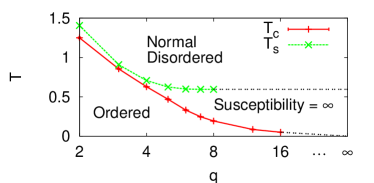
Figure 2: (Color online) Phase diagram of the $q$-state clock model on the heptagonal lattice as shown in Fig. 1. We define two transition temperatures $T_{c}$ and $T_{s}$ so that there exist the ordered phase below $T_{c}$ and the normal disordered phase above $T_{s}$. The intermediated phase is characterized by a diverging susceptibility with no magnetic order. The dotted lines mean extrapolated behaviors of the transition temperatures to the $XY$-model limit ($q=\infty$).

In Fig. 2, we propose a phase diagram of the clock model on the physically realizable hyperbolic lattice introduced in Sec. II. In this diagram, we define $T_{c}$ as the temperature above which the magnetic order vanishes. Apart from the ordered and disordered phases, we can identify the third intermediate one, which is also disordered but exhibits a diverging susceptibility. Therefore, we specify one more transition temperature denoted as $T_{s}$, above which the susceptibility divergence disappears and the normal disordered phase begins.

In order to obtain the phase diagram, we employ the parallel tempering method exchange and measure the magnetic order parameter

$$\left<|m|\right>=\left<\left|\frac{1}{N}\sum_{j}e^{i\theta_{j}}\right|\right>,$$

where $\left<\cdots\right>$ represents the thermal average. From Binder’s fourth-order cumulant binder ,

$$U_{N}(T)=1-\frac{\left<|m|^{4}\right>}{3\left<|m|^{2}\right>^{2}}$$

for different $l$, we can locate a unique crossing point for each $q$ [Figs. 3(a)-3(c)]. This determines the lower transition temperature $T_{c}$ as a function of $q$.

Figure 3(d) shows the dependence of $T_{c}$ on $q$. $T_{c}$ is found to rapidly decrease to zero as $q$ grows larger. A striking observation is that $T_{c}$ is determined by the typical energy scale $\Delta E$ to rotate a spin in the fully ordered ground state. $\Delta E$ is roughly given by

$$\Delta E\propto 1-\cos\left(\frac{2\pi}{q}\right)=\sin^{2}\left(\frac{\pi}{q}\right)$$ (8)

in units of $J/k_{B}$ [see Eq. (1)], being proportional to $T_{c}$ for each $q$ as clearly shown in Fig. 3(d). In addition, Eq. (8) can be approximated by $T_{c}\propto 1/q^{2}$ for large $q$, which is analogous to the planar case. More interesting is the fact that the relation of $T_{c}\propto\Delta E$ captures the exact relation, $T_{c}(q=4)=\frac{1}{2}T_{c}(q=2)$, mentioned in the previous section. These results are consistent with the interpretation that the spin-wave excitation breaks every magnetic order in the $XY$ model xy ; in fact, Eq. (8) leads to $\Delta E=0$ in the limit of $q\to\infty$, and thus $T_{c}=0$.

It is worthy to mention the significant contribution of boundary spins to the determination of $T_{c}$; this is caused by the fact that the actual magnitude of $\Delta E$ depends on the number of neighbors. Since boundary spins have fewer neighbors, the proportionality constant in Eq. (8) takes a smaller value than those of bulk spins so that their orientation will be strongly disturbed by thermal fluctuations. We also comment that the spin-wave excitation is observable in the hyperbolic lattice without boundary since it is the basic excitation mode. In the latter system, however, the excitation is not sufficient to destroy the ordered phase but arises as a separate peak in specific heat at $q>4$ gendiar .

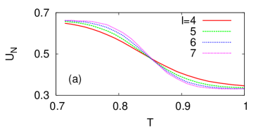
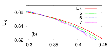
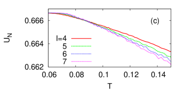
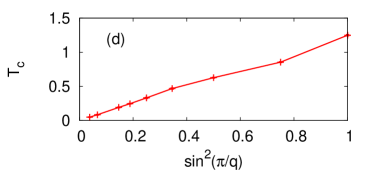
Figure 3: (Color online) Binder’s fourth-order cumulant for the $q$-state clock model on heptagonal lattices with (a) $q=3$, (b) $q=6$, and (c) $q=12$. (d) Transition temperatures between the ordered and disordered phases, $T_{c}$, compared to $\sin^{2}(\pi/q)$.

Figure 4: Distributions of the magnetic order parameter for Ising spin systems ($q=2$) (a) in a heptagonal lattice and (b) in a plane. To compare these two cases, we make both systems have sizes of $N\sim O(10^{3})$, and set $T\approx 0.8~{}T_{c}$ to observe low-temperature regions. A narrow Gaussian peak is clearly shown in the planar case while a longer tail is observed at low $|m|$ in the heptagonal case auriac .

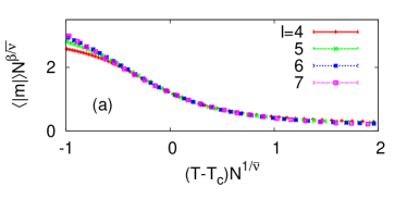
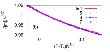
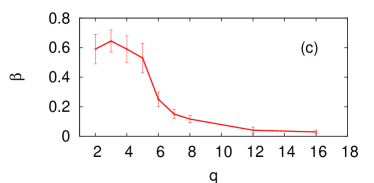
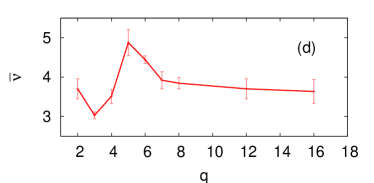
Figure 5: (Color online) Finite-size scaling using Eq. (9) for (a) $q=4$ and (b) $q=16$. Here the parameters are chosen as $\beta/\bar{\nu}=0.167$, $1/\bar{\nu}=0.285$, and $T_{c}=0.63$ for $q=4$, and $\beta/\bar{\nu}=0.0075$, $1/\bar{\nu}=0.275$, and $T_{c}=0.05$ for $q=16$. By this way, we estimate behaviors of critical indices (c) $\beta$ and (d) $\bar{\nu}$ as $q$ varies.

III.3 Two distinct scaling relations around $T_{c}$ and $T_{s}$

We next evaluate critical exponents of the transition by employing the finite-size scaling analysis. As pointed out in Ref. auriac , distribution functions of $|m|$ for the heptagonal lattice deviate from the Gaussian distributions (Fig. 4). Since the idea of the fourth-order cumulant assumes a Gaussian peak shape binder , a direct scaling of the cumulant will give a different value from the actual correlation-length exponent estimated from the order parameter shima . In order to find an appropriate estimate, therefore, we perform at each $q$ the scaling analysis for $\left<|m|\right>$ based on the scaling hypothesis:

$$\left<|m|\right>\propto N^{-\beta/\bar{\nu}}f\left(|T-T_{c}|N^{1/\bar{\nu}}\right).$$ (9)

In the present case, we choose $N$ instead of $l$ as a proper scaling variable, as $N$ gives much better scaling collapse at $T_{c}$ than $l$. Although the finite-size scaling of the Binder’s cumulant with $\bar{\nu}$ fails due to the non-Gaussian nature of the magnetization distribution, $T_{c}$’s estimated from the crossing of $U_{N}$ and from Eq. (9) are almost identical. Figure 5 shows the resulting scaling plots and estimated critical exponents as functions of $q$. While $\bar{\nu}$ appears to be relatively constant at $q>6$, $\beta$ tends to decrease to zero, suggesting that that every $q$-state clock model belongs to a different universality class, apart from the exact equivalence between $q=2$ and $4$.

Measuring the magnetic susceptibility $\chi=N(\left<|m|^{2}\right>-\left<|m|\right>^{2})/k_{B}T$ usually gives another way to estimate $\bar{\nu}$ with a similar scaling hypothesis,

$$\chi\propto N^{-\gamma/\bar{\nu}}f\left(|T-T_{c}|N^{1/\bar{\nu}}\right).$$ (10)

This yields consistent results with the above ones for $q\leq 4$, and confirms the results in Ref. shima for $q=2$ and $4$. However, we find Eq. (10) inapplicable at $q>4$ to obtain critical indices since the susceptibility begins to diverge at a temperature $T_{s}$, much higher than $T_{c}$. In contrast, the length scale $l$ successfully works as a scaling variable (Fig. 6). Henceforth, we should employ the following alternative scaling hypothesis around $T_{s}$,

$$\chi\propto l^{-\gamma^{\prime}/\nu}g(|T-T_{s}|~{}l^{1/\nu}),$$ (11)

which locates the phase-separation point $T_{s}$ as depicted in Fig. 2. In a usual $d$-dimensional lattice, there exists a trivial relationship between exponents found in Eqs. (10) and (11), derived from $N\sim l^{d}$. In absence of such a relation between $N$ and $l$, it is rather nontrivial to observe these different scalings in a single system at different temperatures. A similar change in the scaling variable across two transitions is also found in percolation phenomena on hyperbolic lattices perc .

It is noticeable that a diverging susceptibility at finite $T_{s}$ appears to be the counterpart of the susceptibility divergence at $T_{\rm KT}$ in the planar $XY$ model. More interestingly, the higher transition temperature $T_{s}$, separate from $T_{c}$, exists for all $q$ for the heptagonal lattice, whereas the quasiliquid phase in the planar case does not appear with $q\leq 4$. To look into its origin, we below examine the clock model on the Cayley tree.

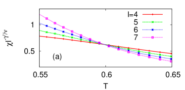
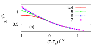
Figure 6: (Color online) Susceptibility scaling with $l$ in case of $q=6$. (a) The crossing point at $T_{s}=0.6$ with $\gamma^{\prime}/\nu=2$, and (b) scaling collapse with $1/\nu=1.5$.

III.4 Comparison with Cayley tree

The Cayley tree is a special type of hyperbolic lattices containing no loops, which often allows exact calculations as a useful guidance. In order to understand the existence of the intermediate phase, we extend the results for the Ising model ($q=2$) on the Cayley tree, presented in Refs. stosic1 and stosic2 , to general $q$.

Let us consider a branching number of $B=2$, i.e., a binary tree with $n$ generations, where a root node is denoted as the zeroth generation. The total number of nodes are $N_{n}=2^{n+1}-1$. Let $Z_{n}^{(\theta)}$ denote the partition function of this branch, restricted that the root node has a phase variable as $\theta$. The complete partition function would be then $Z_{n}=\sum_{\theta}Z_{n}^{(\theta)}$, where the summation $\sum_{\theta}$ runs over $\theta=0,\frac{2\pi}{q},\frac{4\pi}{q},\ldots,\frac{2\pi(q-1)}{q}$. A tree with $(n+1)$ generations can be generated by attaching two trees with $n$ generations to a single node, which has a certain angle $\theta$. Since two $n$-generation trees are totally independent, one can write the following recursion relation,

$$Z_{n+1}^{(\theta)}=e^{\bar{\beta}h\cos\theta}\left[\sum_{\theta^{\prime}}Z_{n}^{(\theta^{\prime})}e^{\bar{\beta}J\cos(\theta-\theta^{\prime})}\right]^{2},$$ (12)

where $\bar{\beta}\equiv(k_{B}T)^{-1}$ and the magnetic field $h$ is assumed to be in parallel with $\theta=0$.

By differentiating Eq. (12) and taking the limit as $h\rightarrow 0$ (see Appendix A), we find the magnetization of the $n$-generation tree with broken symmetry as follows:

$$\left<m\right>_{n} = \frac{1}{N_{n}}\frac{1}{Z_{n}^{(0)}}\frac{\partial Z_{n}^{(0)}}{\partial(\bar{\beta}h)}=\frac{1}{N_{n}}\sum_{j=0}^{n}(2R)^{j}$$ (13)

$$= \frac{1}{2^{n+1}-1}\frac{(2R)^{n+1}-1}{2R-1},$$

where $R\equiv\left[\sum_{\theta}e^{\bar{\beta}J\cos\theta}\cos\theta\right]/\left[\sum_{\theta}e^{\bar{\beta}J\cos\theta}\right]$. Following the argument in Ref. falk , we remark that the correlation between a pair of spins, separated by the distance $r$, is given as $R^{r}$. Since $R<1$ in general, the magnetization $\left<m\right>_{n}$ goes to zero as $n\rightarrow\infty$. One may also consider the free-energy cost of forming a spin cluster on a subbranch of this tree. Since a single bond divides the whole tree into two regions, the energy cost at the interface is $\delta E=2\left[1-\cos(2\pi/q)\right]$, basically constant regardless of the cluster size. At any finite temperatures, the entropy gain $\delta S$, by forming a spin cluster, will thus dominate the free-energy change, readily breaking the magnetic order (see Ref. melin for a typical spin configuration). Yet one should note that this large-system limit can be quite subtle stosic3 .

The second-order derivative of Eq. (12) leads to (see Appendix C)

$$\chi_{n} = \frac{\bar{\beta}}{N_{n}}\left[\frac{1}{Z_{n}}\frac{\partial^{2}Z_{n}}{\partial(\bar{\beta}h)^{2}}-\left(\frac{1}{Z_{n}}\frac{\partial Z_{n}}{\partial(\bar{\beta}h)}\right)^{2}\right]\simeq\frac{\bar{\beta}}{N_{n}q}\sum_{\theta}\frac{1}{Z_{n}^{(\theta)}}\frac{\partial^{2}Z_{n}^{(\theta)}}{\partial(\bar{\beta}h)^{2}}$$

$$= \frac{\bar{\beta}S}{(2^{n+1}-1)q}\left\{\frac{(R+1)^{2}2^{n+1}}{1-2R^{2}}+\frac{4R^{4}}{2R^{2}-1}\left[\sum_{j=0}^{n-1}(2R)^{j}\right]^{2}+\frac{2R+1}{2R^{2}-1}\sum_{j=0}^{n+1}(2R)^{j}\right\},$$

where $S\equiv\sum_{\theta}\cos^{2}\theta$. This formula recovers the Ising case with $q=2$, where $\chi_{n}$ diverges at $\bar{\beta}_{s}J\equiv J/k_{B}T_{s}=\ln(1+\sqrt{2})\approx 0.8814$ stosic2 . Also in general, Eq. (III.4) diverges at $R=1/\sqrt{2}$. If $q\rightarrow\infty$, we may rewrite the summations in $R$ as integrals so that $R=\left[\int_{0}^{2\pi}e^{\bar{\beta}J\cos\theta}\cos\theta\right]/\left[\int_{0}^{2\pi}e^{\bar{\beta}J\cos\theta}\right]=I_{1}(\bar{\beta}J)/I_{0}(\bar{\beta}J)$, where $I_{n}(x)$ is the modified Bessel function of the first kind. A numerical solution then gives $\bar{\beta}_{s}J\approx 2.0582$. Since $\chi_{n}(R)$ is basically the same at any $q$ and $R$ is always a monotonic function of temperature, the divergence should be also qualitatively the same as in $q=2$. That is, susceptibility diverges as $\chi_{n}/n\sim a_{0}+a_{1}(T-T_{s})n$ with some constants $a_{0}$ and $a_{1}$ stosic2 .

The susceptibility divergence can be explained by the presence of boundaries falk . From the viewpoint of boundary spins, which dominate the overall property, the effective number of generations appears as $n^{\prime}\simeq 2n$ since it is the maximum possible distance in this tree. Therefore, the effective branching number for a boundary spin amounts to $\tilde{B}\simeq\sqrt{2}$ so that $\tilde{B}^{n^{\prime}}=N\sim 2^{n}$ (see Ref. auriac for a general discussion). According to Eq. (7), the contribution of each boundary spin to susceptibility is roughly $C=\sum_{j}^{n^{\prime}}\tilde{B}^{j}R^{j}$. Since the number of boundary spins is proportional to the system size $N$, we find the lower bound of susceptibility that $\chi_{n}\geq\bar{\beta}C$, and expectedly this will make the most dominant term. At $R=1/\sqrt{2}$, we have $\tilde{B}R\simeq 1$, which means that $C\simeq\sum^{2n}O(1)$. Note that the summation is limited by the number of generations, $n$. In other words, the susceptibility diverges with $\chi_{n}\propto n$ at $R=1/\sqrt{2}$.

Recalling differences between with and without loops in percolation phenomena perc , we may expect only a qualitative understanding for the heptagonal lattice from studying the Cayley tree rather than a quantitative agreement. Although the presence of closed loops will presumably alter the results described above, the essential parts of these arguments could be conveyed to our heptagonal lattice. That is, the susceptibility divergence at $T_{s}$ should be attributed to the exponential growth of $N(l)$. This is markedly different from the case in regular lattices, where the susceptibility divergence is due to divergence in the correlation length. In particular, the correlations among boundary spins play the most important role at this point. Nonetheless, the correlation function does not have to decay algebraically yet, which is a possible reason that Binder’s cumulant does not detect $T_{s}$. One cannot observe the algebraic decay until reaching $T_{c}(<T_{s})$. Around that point, the hyperbolic lattice begins to manifest itself more as a surface. In contrary to the tree case above, for example, the energy cost at a domain wall increases roughly logarithmically with the cluster size perc , opening the possibility for $T_{c}$ to be finite. As a consequence, we observe these three phases in general: an ordered phase, a disordered phase but having a diverging susceptibility, and a normal disordered phase with a finite susceptibility.

IV Summary

We investigated the $q$-state clock model on the heptagonal lattice, and found that the spin-wave excitation is relevant in the order-disorder transition in this system. In the planar $q$-state clock model, one could expect one additional quasiliquid phase, and thus two phase transitions for $q>4$. The lower transition defines the line between true- and quasi-long-range order, and the higher one defines where the quasi-long-range order vanishes. If we only introduce the curvature effect but without the finite surface-volume ratio, the quasi-long-range order becomes a genuine order and the higher transition is of the mean-field type since fluctuation decays exponentially (see Sec III.1). However, the presence of a boundary cannot be neglected, which breaks the mean-field picture, and the spin-wave excitation appears to be crucial in establishing the ordered phase. In the limit of $q\rightarrow\infty$, the excitation becomes gapless so that the transition temperature approaches zero. In addition, the susceptibility begins to diverge at a higher temperature, indicating a similar phenomenon to the KT transition with a diverging susceptibility. By analyzing the clock model on the Cayley tree, we suggest that the hyperbolic nature of the underlying lattice structure makes the third phase observable for every $q\geq 2$.

Appendix A Magnetization in Cayley Tree

If we take the limit of $h\rightarrow 0$, Eq. (12) leads to

$$Z_{n+1}^{(\theta)}={Z_{n}^{(\theta)}}^{2}\left[\sum_{\theta^{\prime}}e^{\bar{\beta}J\cos(\theta-\theta^{\prime})}\right]^{2},$$ (15)

since $Z_{n}^{(\theta)}=Z_{n}^{(\theta=0)}$ by symmetry. It is straightforward to see that

$$Z_{n}^{(\theta)}=\left[\sum_{\theta^{\prime}}e^{\bar{\beta}J\cos\theta^{\prime}}\right]^{2N_{n}},$$ (16)

since

$$\sum_{\theta^{\prime}}e^{\bar{\beta}J\cos(\theta-\theta^{\prime})}=\sum_{\theta^{\prime}}e^{\bar{\beta}J\cos\theta^{\prime}}.$$ (17)

Note that Eq. (16) is an analytic function at any $T$ egg . As to derivatives, one finds the following equations by differentiating Eq. (12) with respect to $\bar{\beta}h$:

$$\frac{\partial Z_{n+1}^{(\theta)}}{\partial(\bar{\beta}h)}=Z_{n+1}^{(\theta)}\cos\theta+2e^{\bar{\beta}h\cos\theta}I_{0}I_{1},$$ (18)

where

$$I_{k}(\theta)\equiv\sum_{\theta^{\prime}}\frac{\partial^{k}Z_{n}^{(\theta^{\prime})}}{\partial(\bar{\beta}h)^{k}}e^{\bar{\beta}J\cos(\theta-\theta^{\prime})},\quad[k=0,1,2].$$

We then take the zero-field limit, $h\rightarrow 0$. By mathematical induction (see Appendix B), one can show

$$\frac{\partial Z_{n}^{(\theta)}}{\partial(\bar{\beta}h)}=\frac{\partial Z_{n}^{(\theta=0)}}{\partial(\bar{\beta}h)}\cos\theta.$$ (19)

Henceforth, by Eqs. (15) and (19), we can rewrite Eq. (18) for a restricted ensemble with $\theta=0$ as follows,

$$\frac{1}{Z_{n+1}^{(0)}}\frac{\partial Z_{n+1}^{(0)}}{\partial(\bar{\beta}h)}=1+2\frac{\sum_{\theta}e^{\bar{\beta}J\cos\theta}\cos\theta}{\sum_{\theta}e^{\bar{\beta}J\cos\theta}}\frac{1}{Z_{n}^{(0)}}\frac{\partial Z_{n}^{(0)}}{\partial(\bar{\beta}h)},$$ (20)

which directly leads to Eq. (13).

Appendix B Mathematical Induction

Let us assume that Eq. (19) holds true, as it does for $n=0$,

$$\left.\frac{\partial Z_{0}^{(\theta)}}{\partial(\bar{\beta}h)}\right|_{h=0}=\left.e^{\bar{\beta}h\cos\theta}\cos\theta\right|_{h=0}=\cos\theta.$$

Then for general $n$, this assumption yields the following relation:

$$\frac{\partial Z_{n+1}^{(\theta)}}{\partial(\bar{\beta}h)}=Z_{n+1}^{(\theta)}\cos\theta+2Z_{n}^{(\theta)}\frac{\partial Z_{n}^{(\theta=0)}}{\partial(\bar{\beta}h)}\left[\sum_{\theta^{\prime}}e^{\bar{\beta}J\cos(\theta-\theta^{\prime})}\right]\left[\sum_{\theta^{\prime}}e^{\bar{\beta}J\cos(\theta-\theta^{\prime})}\cos\theta^{\prime}\right].$$ (21)

Here we note the following identity:

$$\sum_{\theta^{\prime}}e^{\bar{\beta}J\cos(\theta-\theta^{\prime})}\cos\theta^{\prime} = \sum_{\theta^{\prime\prime}}e^{\bar{\beta}J\cos\theta^{\prime\prime}}\cos(\theta-\theta^{\prime\prime})$$ (22)

$$= \cos\theta\sum_{\theta^{\prime\prime}}e^{\bar{\beta}J\cos\theta^{\prime\prime}}\cos\theta^{\prime\prime}+\sin\theta\sum_{\theta^{\prime\prime}}e^{\bar{\beta}J\cos\theta^{\prime\prime}}\sin\theta^{\prime\prime}$$

$$= \cos\theta\sum_{\theta^{\prime\prime}}e^{\bar{\beta}J\cos\theta^{\prime\prime}}\cos\theta^{\prime\prime},$$

where $\theta^{\prime\prime}\equiv\theta-\theta^{\prime}$ and the last equality is due to the fact that $\sin\theta^{\prime\prime}$ is an odd function. Therefore, we substitute Eqs. (17) and (22) into Eq. (21) and then obtain

$$\frac{\partial Z_{n+1}^{(\theta)}}{\partial(\bar{\beta}h)} = \left\{Z_{n+1}^{(\theta=0)}+2Z_{n}^{(\theta=0)}\frac{\partial Z_{n}^{(\theta=0)}}{\partial(\bar{\beta}h)}\left[\sum_{\theta^{\prime}}e^{\bar{\beta}J\cos\theta^{\prime}}\right]\left[\sum_{\theta^{\prime}}e^{\bar{\beta}J\cos\theta^{\prime}}\cos\theta^{\prime}\right]\right\}\cos\theta$$

$$= \frac{\partial Z_{n+1}^{(\theta=0)}}{\partial(\bar{\beta}h)}\cos\theta,$$

which confirms Eq. (19) for any $n\geq 0$.

Appendix C Susceptibility in Cayley Tree

For describing susceptibility, we again differentiate Eq. (18) to get

$$\frac{\partial^{2}Z_{n+1}^{(\theta)}}{\partial(\bar{\beta}h)^{2}} = \frac{\partial Z_{n+1}^{(\theta)}}{\partial(\bar{\beta}h)}\cos\theta+2e^{\bar{\beta}h\cos\theta}\left(\cos\theta I_{0}I_{1}+I_{1}^{2}+I_{0}I_{2}\right).$$ (23)

In the zero-field limit, we have the following:

$$\frac{1}{Z_{n+1}^{(\theta)}}\frac{\partial^{2}Z_{n+1}^{(\theta)}}{\partial(\bar{\beta}h)^{2}} = (1+4R)\cos^{2}\theta\frac{1}{Z_{n}^{(0)}}\frac{\partial Z_{n}^{(0)}}{\partial(\bar{\beta}h)}+2R^{2}\cos^{2}\theta\left[\frac{1}{Z_{n}^{(0)}}\frac{\partial Z_{n}^{(0)}}{\partial(\bar{\beta}h)}\right]^{2}+2\frac{\sum_{\theta^{\prime}}\frac{1}{Z_{n}^{(\theta^{\prime})}}\frac{\partial^{2}Z_{n}^{(\theta^{\prime})}}{\partial(\bar{\beta}h)^{2}}e^{\bar{\beta}J\cos(\theta-\theta^{\prime})}}{\sum_{\theta^{\prime}}e^{\bar{\beta}J\cos\theta^{\prime}}}.$$

To simplify the last term, we sum up both sides over $\theta$ and find

$$\sum_{\theta}\frac{1}{Z_{n+1}^{(\theta)}}\frac{\partial^{2}Z_{n+1}^{(\theta)}}{\partial(\bar{\beta}h)^{2}}=S\left\{(1+4R)\frac{1}{Z_{n}^{(0)}}\frac{\partial Z_{n}^{(0)}}{\partial(\bar{\beta}h)}+2R^{2}\left[\frac{1}{Z_{n}^{(0)}}\frac{\partial Z_{n}^{(0)}}{\partial(\bar{\beta}h)}\right]^{2}\right\}+2\sum_{\theta}\frac{1}{Z_{n}^{(\theta)}}\frac{\partial^{2}Z_{n}^{(\theta)}}{\partial(\bar{\beta}h)^{2}},$$ (24)

where $S\equiv\sum_{\theta}\cos^{2}\theta$. Now Eq. (24) describes the full ensemble without breaking symmetry, which is valid above criticality. The terms inside the curly brackets can be explicitly written by using Eq. (13). Solving this recursion relation with the first term as

$$\sum_{\theta}\frac{1}{Z_{0}^{(\theta)}}\frac{\partial^{2}Z_{0}^{(\theta)}}{\partial(\bar{\beta}h)^{2}}=\sum_{\theta}\cos^{2}\theta=S,$$

we obtain Eq. (III.4) as the susceptibility for the $n$-generation tree.

References

- (1) N. L. Balazs and A. Voros, Phys. Rep. 143, 109 (1986).
- (2) D. Vanderbilt and J. Tersoff, Phys. Rev. Lett. 68, 511 (1992); N. Park, M. Yoon, S. Berber, J. Ihm, E. Osawa, and D. Tománek, ibid. 91, 237204 (2003).
- (3) R. D. Kamien, Rev. Mod. Phys. 74, 953 (2002); V. Vitelli and A. M. Turner, Phys. Rev. Lett. 93, 215301 (2004); J. L. van Hemmen and C. Leibold, Phys. Rep. 444, 51 (2007).
- (4) H. Shima and Y. Sakaniwa, J. Phys. A 39, 4921 (2006).
- (5) K. Ueda, R. Krcmar, A. Gendiar, and T. Nishino, J. Phys. Soc. Jpn. 76, 084004 (2007).
- (6) S. K. Baek, P. Minnhagen, and B. J. Kim, Europhys. Lett. 79, 26002 (2007).
- (7) J. C. A. d’Auriac, R. Mélin, P. Chandra, and B. Douçot, J. Phys. A 34, 675 (2001).
- (8) H. Shima and Y. Sakaniwa, J. Stat. Mech.: Theory Exp. P08017 (2006).
- (9) S. K. Baek, S. D. Yi, and B. J. Kim, Phys. Rev. E 77, 022104 (2008).
- (10) S. K. Baek, P. Minnhagen, and B. J. Kim, Phys. Rev. E 79, 011124 (2009).
- (11) S. K. Baek, H. Shima, and B. J. Kim, Phys. Rev. E 79, 060106(R) (2009).
- (12) F. Sausset and G. Tarjus, J. Phys. A: Math. Theor. 40, 12873 (2007); F. Sausset, G. Tarjus, and P. Viot, Phys. Rev. Lett. 101, 155701 (2008).
- (13) L. R. A. Belo, N. M. Oliveira-Neto, W. A. Moura-Melo, A. R. Pereira, and E. Ercolessi, Phys. Lett. A 365, 463 (2007).
- (14) A. Gendiar, R. Krcmar, K. Ueda, and T. Nishino, Phys. Rev. E 77, 041123 (2008).
- (15) R. Krcmar, T. Iharagi, A. Gendiar, and T. Nishino, Phys. Rev. E 78, 061119 (2008).
- (16) H. S. M. Coxeter, Can. Math. Bull. 40, 158 (1997).
- (17) M. J. Greenberg, Euclidean and Non-Euclidean Geometries: Development and History, 3rd ed. (W. H. Freeman and Company, New York, 1993).
- (18) F. Y. Wu, Rev. Mod. Phys. 54, 235 (1982).
- (19) M. Suzuki, Prog. Theor. Phys. 37, 770 (1967).
- (20) C. M. Lapilli, P. Pfeifer, and C. Wexler, Phys. Rev. Lett. 96, 140603 (2006).
- (21) V. L. Berezinskii, Sov. Phys. JETP 32, 493 (1971); J. M. Kosterlitz and D. J. Thouless, J. Phys. C 6, 1181 (1973).
- (22) S. Elitzur, R. B. Pearson, and J. Shigemitsu, Phys. Rev. D 19, 3698 (1979).
- (23) J. V. Jose, L. P. Kadanoff, S. Kirkpatrick, and D. R. Nelson, Phys. Rev. B 16, 1217 (1977).
- (24) F. Liu and G. F. Mazenko, Phys. Rev. B 47, 2866 (1993); A. J. Bray, Adv. Phys. 43, 357 (1994).
- (25) Y. Enomoto and R. Kato, J. Phys.: Condens. Matter 2, 9215 (1990).
- (26) E. C. Young, Vector and Tensor Analysis, 2nd ed. (Marcel Dekker, New York, 1993).
- (27) N. Goldenfeld, Lectures on Phase Transitions and the Renormalization Group (Addison-Wesley, Reading, MA, 1992).
- (28) J. Viana Lopes, Y. G. Pogorelov, J. M. B. Lopes dos Santos, and R. Toral, Phys. Rev. E 70, 026112 (2004).
- (29) K. Hukushima and K. Nemoto, J. Phys. Soc. Jpn. 65, 1604 (1996).
- (30) K. Binder and D. W. Heermann, Monte Carlo Simulation in Statistical Physics, 2nd ed. (Springer-Verlag, Berlin, 1992).
- (31) T. Stošić, B. Stošić, and I. P. Fittipaldi, J. Magn. Magn. Mater. 177-181, 185 (1998).
- (32) T. Stošić, B. Stošić, and I. P. Fittipaldi, Physica A 320, 443 (2003).
- (33) H. Falk, Phys. Rev. B 12, 5184 (1975).
- (34) R. Mélin, J. C. A. d’Auriac, , P. Chandra, and B. Douçot, J. Phys. A 29, 5773 (1996).
- (35) B. Stošić, T. Stošić, and I. P. Fittipaldi, Physica A 355, 346 (2005).
- (36) T. P. Eggarter, Phys. Rev. B 9, 2989 (1974).