Topological phase transition in a RNA model

in the de Gennes regime

Matías G. dell’Erba

Instituto de Física de Mar del Plata, IFIMAR (CONICET-UNMdP)

and

Departamento de Física, Facultad de Ciencias Exactas y Naturales, Universidad Nacional de Mar del Plata, Funes 3350, (7600), Mar del Plata, Argentina

Guillermo R. Zemba

Facultad de Ciencias Fisicomatemáticas e Ingeniería, Pontificia Universidad Católica Argentina, Av. A. Moreau de Justo 1500, Buenos Aires, Argentina

and

Departamento de Fısica, C.N.E.A. Av.Libertador 8250, (1429) Buenos Aires, Argentina

We study a simplified model of the RNA molecule proposed by G. Vernizzi, H. Orland and A. Zee in the regime of strong concentration of positive ions in solution. The model considers a flexible chain of equal bases that can pairwise interact with any other one along the chain, while preserving the property of saturation of the interactions. In the regime considered, we observe the emergence of a critical temperature $T_{c}$ separating two phases that can be characterized by the topology of the predominant configurations: in the large temperature regime, the dominant configurations of the molecule have very large genera (of the order of the size of the molecule), corresponding to a complex topology, whereas in the opposite regime of low temperatures, the dominant configurations are simple and have the topology of a sphere. We determine that this topological phase transition is of first order and provide an analytic expression for $T_{c}$. The regime studied for this model exhibits analogies with that for the dense polymer systems studied by de Gennes.

PACS numbers: 87.14gn , 02.10.Yn , 87.15.Cc

1 Introduction

Recent advances in mathematical models of RNA and DNA molecules have led to stimulating new studies of their complex spatial properties and their relation with the environmental variables ( see, e.g. [1, 2, 3, 4, 5] ). In this paper we consider the exactly solved model for a RNA molecule presented in [6], which consists of a homopolymer of length $L$, with an infinitely flexible backbone, and in which any arbitrary pair of bases is allowed to (pairwise) interact. This combinatorial model preserves the important property of saturation of the interactions [2, 7] of the actual RNA molecule, but does not include both the geometric and energetic aspects of the real molecules. Due to its simplicity, the model is exactly solved, i.e., it allows for analytical expressions of statistical and topological interesting quantities, such as the partition function and its topological expansion [8]. A crucial ingredient of the model is the introduction of an extra degree of freedom, $N$, such that a random $N\times N$ hermitian matrix is added to each base position along the chain. A physical interpretation can be given to this parameter a posteriori [6, 8, 9]: $1/N$ plays a role in the model that can be associated to the concentration of positive ions (like $\rm{Mg}^{++}$) in solution for real molecules. These positive ions are responsible for the overall electric charge neutralization of the system compensating the negative charge in the phosphate groups in the RNA molecule. The neutralization of the phosphate ions provide the physical mechanism for the folding of the molecule [10, 11, 12, 13, 14, 15]. Moreover, the algebraic power of $1/N^{2}$ in the topological expansion of the partition function of the model is the genus of the diagrams associated to the different configurations [6, 8, 16]. These diagrams encode the real spatial structure of the molecule, in the sense that they are analogous to the secondary (or planar) structure of the molecule, from which the tertiary (or spatial) one is obtained [6]. Therefore, the parameter $N$ works as a regulator that controls the topology of the molecule within the model. To the best of our knowledge, the regime of $N\to 0$ has not been received much attention in the theoretical models considered in the literature, and in this paper we address some questions arising in this regime. We identify this regime with the dense polymer phase of the $O(n)$ vector model of de Gennes [17], which is described by the limit $n\to 0$. Furthermore, we are not aware of any experimental works in real RNA molecules in the corresponding laboratory regime.

In a previous work [8], we have provided an exact analytic expression for the partition function of the model, which has been used to study its thermodynamic properties in the regime $N\geq 1$, i.e., that of small ion concentration in the surrounding environment. However, some of the expressions that we have obtained in that paper are analytical in $N$ and are, therefore, useful to explore other regimes than the one we have chosen to discuss in that work. In this paper we study (for a wide range of temperatures) the complementary regime $N\to 0$ , which can be characterized as one with large positive ion concentration in the surrounding medium. We observe the emergence of a critical temperature $T_{c}$ separating two regimes with different spatial configurations: in the large temperature regime, the dominant configurations of the molecule have very large genera (of the order of the size of the molecule), corresponding to a complex topology, whereas in the opposite regime of low temperatures, the dominant configurations are simple and have the topology of a sphere. This transition is not related a-priori to the so-called coil-globule transition in which the molecule adopts the shape of an elongated coil for low temperatures, whereas it assumes a compact globule shape in the large temperature regime. This latter transition is considered to be of first order [3, 18, 19, 20, 21].

Some recent work in the literature has recently addressed related issues. In [18], a study of the distribution of genera of pseudoknotted configurations in the $T$-dependent phase transition for a self-avoiding homopolymer on a lattice has been considered. A study of the behavior of the distribution of genera for the model introduced in [6] with external perturbations has been the subject of Refs. [22, 23]. Moreover, in [22], a ‘structural transition’ dependent on the external perturbation has been also discussed.

This paper is organized as follows: in Section 2 we reconsider the model presented in [6] and recall some exact results, such as the partition function and its topological expansion [8]. Section 3 is devoted to the study of the regime $N\to 0$ and the topological phase transition: we first consider the mathematical setting and approximations that are needed to analytically treat the phase transition. We then apply this preliminary study to the partition function of the model to make explicit the emergence of the phase transition and we give an analytic expression for the critical temperature. In section 4, we discuss the thermodynamic properties of the system in the limit $N\to 0$. We calculate the free energy per particle, the entropy and the latent heat. From the last thermodynamic quantity, we show that the phase transition is of first order. Finally, we give our conclusions.

2 Topological expansion of the partition function

We start by reviewing some of the properties of the model proposed by G. Vernizzi, H. Orland and A. Zee [6]. The model considers a chain of bases of one type only, such that the interaction energy between any pair of bases is a constant $\epsilon$. A given base can interact with any other base in the chain, but preserving the saturation property, which excludes interactions among three or more bases. We consider that this property is one of the essential ingredients of the simplified model. Therefore, all the Boltzmann factors $v=\exp{(-\epsilon/\kappa T)}$ (where $T$ is the absolute temperature and $\kappa$ is the Boltzmann constant) are equal as well. At each base site, a random $N\times N$ hermitian matrix is added as the relevant degree of freedom. We consider this feature to be a second essential ingredient of the model. The configurational partition function $Z$ of a chain of length $L$ is:

$$Z(L,N,T) = \frac{1}{N}\langle{\rm tr}(1+\frac{1}{L^{1/2}}\varphi)^{L}\rangle$$ (2.1)

$$= \int d\varphi\ e^{-\frac{N}{2Lv}{\rm tr}\varphi^{2}}\frac{1}{N}{\rm tr}(1+\frac{1}{L^{1/2}}\varphi)^{L}{\large/}{\int d\varphi\ e^{-\frac{N}{2Lv}{\rm tr}\varphi^{2}}},$$ (2.2)

where $\varphi$ represents a collective degree of freedom (a sort of center-of-mass random matrix). The simple form of (2.2) is a consequence of the symmetry of the matrix potential that reduces the original integration over $L$ matrices to one integration over $\varphi$ [6]. Applying standard results of random matrices to (2.2) one obtains:

$$Z(L,N,T)=\sum_{k=0}^{[L/2]}d_{k}(L,N)\ e^{-\epsilon_{k}/\kappa T}\ ,$$ (2.3)

where the symbol $[L/2]$ means the integer part of $L/2$, $\epsilon_{k}=k\epsilon$ and

$$d_{k}(L,N)=\sum_{j=0}^{k}\left(\begin{array}[]{c}L\\ 2k\\ \end{array}\right)\left(\begin{array}[]{c}k\\ j\\ \end{array}\right)\left(\begin{array}[]{c}N\\ j+1\\ \end{array}\right)\frac{(2k)!}{2^{k-j}\ k!\ N^{k+1}}\ .$$ (2.4)

From (2.3) we may compute $Z$ exactly (for each $L$), as a function of $N$ and $T$. The spectrum of the system has $[L/2]+1$ energy levels, with energies: $0,\epsilon,2\epsilon,\ldots,[L/2]\epsilon$ and the degeneracy of the $k-th$ level is $d_{k}(L,1)$.

As we have mentioned before, the power of $1/N^{2}$ yields the genus $g$ of the diagram obtained from the chain by joining all interacting bases by a ‘photonic line’ [6], that is, the minimum number of handles of the surface on which the diagram can be drawn without crossings. In [8], we have written the partition function of the model in the form of a topological expansion [16, 6, 2],i.e., as a power series in $1/N^{2}$, where the coefficients take into account all the Feynman diagrams with the same topological character:

$$Z(L,N,T)=\sum_{g=0}^{\infty}z_{g}(L,T)\frac{1}{N^{2g}}\ .$$ (2.5)

Here $z_{g}(L,\infty)$ is the number of planar diagrams that can be drawn on a topological surface of genus $g$ for a molecule of size $L$. Note that, as a function of $T$, $z_{g}(L,T)$ is the partition function of the system living on the topological surface of genus $g$. The coefficients $z_{g}(L,T)$ are given by:

$$z_{g}(L,T)=\sum_{k=0}^{[L/2]}\sum_{j=k-2g}^{k}\frac{L!\ 2^{j-k}\ S_{j+1}^{(k+1-2g)}}{(L-2k)!\ (k-j)!\ j!\ (j+1)!}\ e^{-\epsilon_{k}/\kappa T}\ ,$$ (2.6)

where $S_{j}^{(m)}$ is the Stirling number of the first kind [24, 25] with parameters $m,j$ ($S_{j}^{(m)}=0$ if $m>j$ or if $j\leq 0$). In the limit $T\rightarrow\infty$, $z_{g}(L,T)$ coincides with the coefficients $a_{L,g}$ of Ref. [6]. Using the property of the Stirling numbers mentioned in this paragraph, we see from (2.6) that the maximum genus of a diagram for a given $L$ is $[L/4]$ and, therefore, $g\leq[L/4]$.

3 The partition function in the limit $N\to 0$

3.1 Preliminary study of the analytic behavior of the partition function

In a previous paper, we have considered the limit $N\to\infty$ of the partition function (2.3) [8], for which we gave explicit expressions. As a consequence, we have verified the consistency of interpreting the parameter $1/N$ as being proportional to the density of positive ions in the media surrounding the molecule, as has been suggested in [6]. Therefore, the range of the analysis considered in [8] applies to media with small concentration of positive ions. It is natural to consider as well the opposite situation of large positive ion concentration in the surrounding medium, which corresponds to the limit $N\to 0$. We are going to show later on that this regime is characterized by the existence of a critical temperature and a phase transition.

From the mathematical point of view, studying this limit requires a careful handling of the partition function considered as an analytic function of several variables. Here we discuss a mathematical scheme that allows us to obtain simple analytic expressions in this limit. We first consider a general function $\phi$ of two variables $N$ and $T$ (which will be ultimately related to the free energy) which admits a decomposition of the form:

$$\phi(N,T)=\phi_{f}(T)+\phi_{s}(N,T)\ ,$$ (3.1)

where $\phi_{f}$ ($f$ means ‘fast’) indicates a function whose asymptotic grow in the variable $T$ is in the class of the exponential function, whereas the function $\phi_{s}$ ($s$ means ‘slow’) denotes a function that grows slower than the class of the exponential function (e.g., polynomial, logarithmic classes). Depending on the value of $N$ (which we consider fixed at $N_{0}$) there exists a small range of values of $T$ for which $O(\phi_{f}(T))=O(\phi_{s}(N_{0},T))$ for values of $T$ nearby a critical value $T_{c}$. At this point we can anticipate the idea of defining the critical parameter $T_{c}$ as the value of $T$ for which both the slow and fast parts of the function $\phi$ become equal. We shall further develop on this idea below. The parameter $T_{c}$ emerges naturally in the case when the function $\phi$ is the free energy where it plays the role of a critical temperature. Given the asymptotic behavior of $\phi_{f}$, as soon as $T$ crosses $T_{c}$, the order of $\phi_{f}$ varies rapidly, increasing or decreasing, depending of the sense in which $T$ crosses $T_{c}$, so that (for example):

$$\phi(N_{0},T>T_{c}) \simeq \phi_{f}(T)\ ,$$ (3.2)

$$\phi(N_{0},T<T_{c}) \simeq \phi_{s}(N_{0},T)\ .$$ (3.3)

Therefore, $\phi(N_{0},T)$ has different analytical behavior according to the region in which $T$ is located with respect to $T_{c}$. The change in $\phi$ between these two regions becomes more pronounced when $\phi_{f}$ varies more rapidly. In Fig. 1 we show an example of this behavior for the cases $\phi_{f}=e^{-1/T}$ and $\phi_{s}=NT^{5}$ (in this example $T$ and $N$ are two dimensionless variables) , in the vicinity of $T_{c}\simeq 0.00466$ (the plot has been done numerically): for $T>T_{c}$, $\phi$ is dominated by $\phi_{f}$ and for $T<T_{c}$ it is dominated by $\phi_{s}$.

Figure 1: Plot of $\phi(N,T)=e^{-1/T}+NT^{5}$ around of $T_{c}\simeq 0.00466$ with $N=10^{-80}$.The plot has been done numerically.

If we assume that $\phi_{f}$ is of the form $\phi_{f}(T)\sim e^{-1/T}$, the change is even more noticeable for small values of $T$ . If we had $T_{c}\to 0$, the derivative $\phi^{\prime}(N_{0},T=T_{c})$ would not exist. We shall correlate the absence of the derivative of $\phi$ at the critical point with the appearance of a phase transition of the system for $T_{c}=0$.

3.2 The critical temperature and the phase transition

We now consider the topological expansion in $1/N^{2}$ (2.5) of the partition function $Z$ of the system. Considering that the maximum genus of the diagrams of all possible configurations is $[L/4]$ (as we have mentioned above), we rewrite $Z$ as a polynomial in the variable $N^{2}$ times a $N$-dependent factor which is divergent in the $N\rightarrow 0$ limit:

$$Z(L,N,T) = \frac{1}{N^{2[L/4]}}Z_{R}(L,N,T)\ ,$$ (3.4)

$$Z_{R}(L,N,T) = z_{[L/4]}+z_{[L/4]-1}N^{2}+\cdots+z_{0}N^{2[L/4]}\ .$$ (3.5)

Here the subindex $R$ indicates that the function is regular in the limit $N\rightarrow 0$. The coefficients $z_{g}$ were given in the previous section [8], and can be written as:

$$z_{g}(L,T)=\sum_{k=0}^{[L/2]}r_{k,g}(L)\hskip 2.84544pte^{-k\epsilon/\kappa T},$$ (3.6)

where the coefficients $r_{k,g}(L)$ are given by

$$r_{k,g}(L)=\frac{L!}{(L-2k)!2^{k}}\sum_{j=k-2g}^{k}\frac{2^{j}S_{j+1}^{(k-2g+1)}}{(k-j)!j!(j+1)!}\ ,$$ (3.7)

and $S_{i}^{(j)}$ are the Stirling numbers of the first kind with parameters $i$ and $j$. Using the property $S_{i}^{(0)}=\delta_{i0}$ [26], we rewrite the partition function on the topological surface of genus $[L/4]-n$ as:

$$z_{[L/4]-n}(L,T)=\sum_{k=[L/2]-2n+\delta}^{[L/2]}r_{k,[L/4]-n}(L)\hskip 2.84544pte^{-k\epsilon/\kappa T}\ ,$$ (3.8)

where $\delta=-1$ for $[L/2]$ odd and zero otherwise. Without loss of generality, we shall consider $[L/2]$ even from now on. Substituting the coefficients $z_{g}$ in (3.5), we obtain the regular part of the partition function (RZ):

$$Z_{R}(L,N,T)=e^{-[L/2]\epsilon/\kappa T}\{r_{[L/2],[L/4]}+(r_{[L/2]-2,[L/4]-1}e^{2\epsilon/\kappa T}+r_{[L/2]-1,[L/4]-1}e^{\epsilon/\kappa T}\\ +r_{[L/2],[L/4]-1})N^{2}+\cdots+(r_{0,0}e^{[L/2]\epsilon/\kappa T}\\ +r_{1,0}e^{([L/2]-1)\epsilon/\kappa T}+\cdots+r_{[L/2],0})N^{2[L/4]}\}\ .$$ (3.9)

Note that $r_{0,0}=1$ since it counts the number of configurations with lowest energy and genus, that is, the unique configuration without interaction among bases. In order to treat (3.9) analytically in what follows, we shall consider two approximations on it, valid in the limit $N\ll 1$. We have studied the analytic behavior of (3.9) using the program $Mathematica$ [27], within the range $N\lessapprox 10^{-20}$ in the concrete examples considered. For these examples, the range of sizes of the system is $L\sim 10^{2}-10^{4}$ and that for the temperature is $T\sim 10^{-4}-10^{-2}$.

First, we observe that for the ranges of $L$ and $T$ considered, the terms proportional to $N^{2g}$ are dominated by exponential factors (e.g., $r_{k,g}/r_{k-1,g}\lessapprox 10^{7}$ and $e^{\frac{\epsilon}{\kappa T}}\gtrapprox 10^{43}$ ($\epsilon=\kappa=1$)). For large values of $T$ the most important term in the sum (3.9) is the first one (up to order zero in $N$), whereas for small values of $T$, the dominant term in the sum is the one proportional to $N^{2[L/4]}$ ($=N^{[L/2]}$, for $[L/2]$ even). To keep analytic expressions as simple as possible, we retain only the most important term proportional to $N^{[L/2]}$ in (3.9), i.e., $e^{[L/2]\epsilon/\kappa T}$ and write:

$$Z_{R}(L,N,T)\simeq r_{[L/2],[L/4]}e^{-[L/2]\epsilon/\kappa T}+N^{[L/2]}\ .$$ (3.10)

We refer to (3.10) as the Thermal Approximation (TA) for the partition function, since the relevance of the terms in $Z_{R}$ vary significatively when $T$ crosses $T_{c}$, that is, when $T$ satisfies $O(r_{[L/2],[L/4]}e^{-[L/2]\epsilon/\kappa T})=O(N^{[L/2]})$ (see 3.1).

Next, we specify the definition of $T_{c}$ with more detail. It is clear that (3.10) is a broader approximation to (3.9), since it excludes many terms that are relatively important when the two terms in (3.10) are of the same order, i.e., when $T$ is closer to $T_{c}$. However, we will see later how to minimize the difference between (3.10) and (3.9), showing the conditions under which RZ becomes close to TA. From the TA we calculate the regular part of free energy from $F=-\kappa T\ln Z$:

$$F_{R}(L,N,T)\simeq-\kappa T\ln\{r_{[L/2],[L/4]}e^{-[L/2]\epsilon/\kappa T}+N^{[L/2]}\}\ .$$ (3.11)

In Fig. 2 we show a plot of the thermal approximation for the free energy TA against the temperature. Two regimes can be clearly differentiated, separated by $T=T_{c}$: for $T<T_{c}$, the second term in the logarithm function of (3.11) is much larger than the first one, and can be therefore neglected, with opposite behavior for $T>T_{c}$. These plots show two interesting characteristics: (3.10) behaves linearly below and above $T_{c}$ and the slope for $T<T_{c}$ is higher than that for the case with $T>T_{c}$. We therefore identify a phase transition occurring for $T=T_{c}$, which we identify as the critical temperature. As it is customary for a finite system such as the model for the RNA molecule studied here, the term ‘phase transition’ should be interpreted as a ‘strongly cooperative phenomenon’ [28].

Figure 2: Typical behavior of $F_{R}$ calculated from RZ and TA as a function of $T$ for $L=100$ and $N=10^{-120}$.

In a real RNA molecule, the large negative electric charge of the phosphate ions, prevents it to fold onto a compact structure. The concentration of positive ions in solution, such as $\rm{Mg^{++}}$, neutralize the phosphate ions making possible the folding of the RNA molecule [29, 13, 10]. In the context of the model studied in this paper, if we interpret $1/N$ as the concentration of $\rm{Mg^{++}}$ in solution [8, 2, 9], we see from (3.11) that increasing this concentration favors the formation of RNA structures with large genus, and viceversa.

The asymptotic straight lines in Fig. 2 are obtained by retaining only the leading term in the logarithm of (3.11) when varying the temperature around $T_{c}$. Therefore, the analytic expressions for these asymptotic straight lines are given by:

$$F_{R}\left(L,N,T<T_{c}\right) \simeq -\kappa[L/2]\ln\{N\}T\ ,$$ (3.12)

$$F_{R}\left(L,N,T>T_{c}\right) \simeq -\kappa\ln\{r_{[L/2],[L/4]}\}T+[L/2]\epsilon\ ,$$ (3.13)

and we obtain an analytic expression for the critical temperature equating the two terms in the logarithm of (3.11):

$$T_{c}(L,N)=\frac{\epsilon}{\kappa\ln\left\{(r_{[L/2],[L/4]})^{\frac{1}{[L/2]}}\frac{1}{N}\right\}}$$ (3.14)

As we have mentioned in Sec. 3.1 and show in Fig. 2, the regular free energy $F_{R}$ undergoes a change in its analytic behavior when the temperature reaches the critical value $T_{c}$. Below $T_{c}$, $F_{R}$ is dominated by the slowly varying function ($N^{[L/2]}$), whereas above $T_{c}$, the rapidly varying function ($r_{[L/2],[L/4]}e^{-\frac{[L/2]\epsilon}{\kappa T}}$) dominates. The change in the behavior of $F_{R}$ is sharp in the TA, while for RZ it is obtained for a small range of temperatures because RZ presents additional terms that acquire relative importance when $T$ is close to $T_{c}$.

It can be seen numerically from (3.7) that the function of $L$ in $T_{c}$ behaves linearly as $(r_{[L/2],[L/4]})^{\frac{1}{[L/2]}}=L/e-4.5521$. For large $L$ ($L>200$), we can write the critical temperature as:

$$T_{c}(L,N)\simeq\frac{\epsilon}{\kappa\ln\left(L/eN\right)}\ .$$ (3.15)

Note that (3.15) possess the symmetry $T_{c}(L,N)=T_{c}(aL,aN)$ for $a>0$ a real parameter, that is, $T_{c}$ is scale invariant. Therefore, in the large $L$ limit, we have that $T_{c}(L,N)=T_{c}(L/N)$ Furthermore, there exists a natural cut-off for $N$ such that $T_{c}\geq 0$:

$$N<(r_{[L/2],[L/4]})^{\frac{1}{[L/2]}}\simeq L/e\ .$$ (3.16)

This is a consequence of (3.14) and it is consistent with the condition stating that the slope of the asymptotic straight line for $T<T_{c}$ must be larger than that for $T>T_{c}$. However, this cut-off is not very restrictive because we are interested in the the limit $N\ll 1$ and $L$ is at least of $O(1)$ .

Moreover, there exist further and more restrictive conditions on $N$, implied by both the thermodynamic and large size limits. Given that RZ should approach TA for large $L$, a relationship between $N$ and $L$ should exist. When $L$ increases and $N$ is fixed, the difference between the analytic expressions for RZ and TA also increases. In order to obtain a convergence between the two in the thermodynamic limit, we make $N$ a $L$-dependent variable as follows: for each $L$, there exists an upper limit for $N$ below which the phase transition exists. This can be seen by demanding that the scenario discussed in the previous section actually occurs. For real molecules, this would mean that there should exist a minimal ($L$-dependent) concentration of $\rm{Mg}^{++}$ for which the phase transition exists. As a consequence of this restriction, in the thermodynamic limit $L\to\infty$ then $N\to 0$ , implying $T_{c}\rightarrow 0$. In this limit, the derivative of $F_{R}$ at $T=T_{c}$ (see (3.11)) does not exist and there is a bona fide phase transition.

Furthermore, the limit $N\rightarrow 0$ in the model we have considered can be associated with the dense polymer phase of the $n$ vector model which arises for $n\to 0$ as has been discussed by de Gennes [17]. The correspondence is established between the degrees of freedom of the $O(n)$ vector model, which are $n$-component spin vectors, and the degrees of freedom of the RNA model of [6], given by by $N\times N$ hermitian matrices. The limit $n\rightarrow 0$ in the de Gennes $O(n)$ model corresponds to a high density polymer phase, which is naturally associated to the high concentration of $\rm{Mg}^{++}$ (or other positive ions such as $\rm{K}^{+}$) in solution phase of the RNA model.

From the previous discussion of the RNA model, the $T$-dependent phase transition involves a topology change in the spatial configurations of the molecule, which goes from one with genus zero for $T<T_{c}$ to another one with large genus $[L/4]$ for $T>T_{c}$. The difference in the topology of the configurations of the molecule when $T$ crosses $T_{c}$ justifies the use of the term ‘topological’ for describing the nature of the phase transition. Note that this transition does not correspond to the coil-globule transition in polymers studied in [18], in which the genus of the configurations decreases with increasing temperature (see Fig. 3).

Figure 3: Phase transition between coil and globule states when $T$ crosses $T_{c}$. The arrows indicate the direction in which $T$ increases, to right (left) for high (low) concentration of Mg⁺⁺. This is not to confused with the topological phase transition, as explained in the text.

This is due to the fact that both transitions take place in different regimes: whereas in [18] the RNA molecule is surrounded by a dilute solution of $\rm{Mg}^{++}$, for the case we have discussed the molecule is imbedded in a medium with large concentration of positive ions.

4 Thermodynamic properties in the $N\to 0$ limit

From the analytic results for the partition function obtained in the previous section, we now calculate some thermodynamic quantities that we will use to better describe the configurations of the RNA molecule above and bellow of $T_{c}$ and characterize the nature of the transition that it undergoes. It is important to remark here that the condition $N\ll 1$ (interpreted as meaning a large concentration of Mg⁺⁺) is valid for all the results presented in this section, since this is a necessary condition for using the approximate expression for the partition function instead of the exact one (3.9). In this analysis, we only consider the regular part of the partition function, disregarding the $N$-dependent, divergent factor in (3.5). This factor can be absorbed by convenient renormalizations, and cancels out in any observable quantity which involves an statistical average over the ensemble of random configurations of the system. Therefore, all thermodynamic quantities studied will be, therefore, termed as ‘regular’.

4.1 Free energy per base

From (3.10), we determine the free energy per base, $f=F/L$. Using that $[L/2]/L\rightarrow 1/2$ in the large $L$ limit, we write the regular free energy per base as:

$$f_{R}\left(L,N,T<T_{c}\right) \simeq -\frac{\kappa}{2}\ln\{N\}T$$ (4.1)

$$f_{R}\left(L,N,T>T_{c}\right) \simeq -\frac{\kappa}{2}\ln\{L/e\}T+\frac{\epsilon}{2}\ .$$ (4.2)

On the one hand, from (3.12) we notice that $f_{R}$ is independent of $L$ for $T<T_{c}$. This means that $f_{R}$ is determined by the local (short distances) environment of a point in the chain and not by global (large distances) properties. This behavior is reasonable because thermal agitation is small, which prevents coupling on a given base with another non-neighboring one in the chain. On the other hand, for $T>T_{c}$ we see from (3.13) that $f_{R}$ is in turn independent of $N$. This can be interpreted by noting that for temperatures above $T_{c}$, thermal agitation overcomes the folding action of the positive ion concentration in the medium, rendering the local behavior independent of this concentration, and, therefore, of $N$.

4.2 Entropy

Next, we calculate the regular entropy $S_{R}=-\partial F_{R}/\partial T$ from RZ and TA, and plot it in Fig. 4 , which shows that the dependence of the entropy with the temperature resembles a step function, with a positive step in $T=T_{c}$ (in particular, for the TA case). This behavior could be expected, since $S_{R}(T_{a})\leq S_{R}(T_{b})$ for $T_{a}<T_{b}$ and it is a consequence of the linear asymptotic behavior of the regular free energy displayed in Fig. 2. On the contrary, a negative step in $T=T_{c}$ would have implied $T_{c}<0$. The curves of $S_{R}$ from the TA, for $T$ below and above $T_{c}$, are derived from (3.12) and (3.13). Moreover, it can be seen from Fig. 4 that as $N$ decreases, RZ approaches TA and the behavior of RZ resembles more closely that of a step function:

$$S_{R}\left(L,N,T<T_{c}\right) \simeq \kappa[L/2]\ln\{N\}\ ,$$ (4.3)

$$S_{R}\left(L,N,T>T_{c}\right) \simeq \kappa\ln\{r_{[L/2],[L/4]}\}\simeq\kappa[L/2]\ln\{L/e\}\ .$$ (4.4)

We have verified numerically that, in the limit $N\to 0$, the plot of $S_{R}$ from RZ behaves asymptotically as step function with step in $T_{c}$ of magnitude proportional to the latent heat.

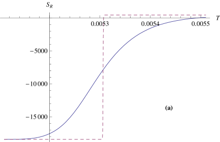
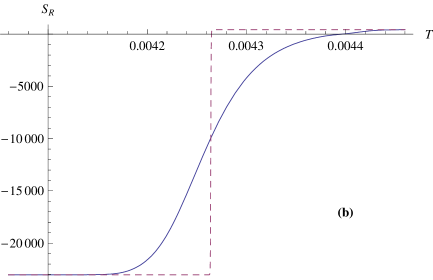
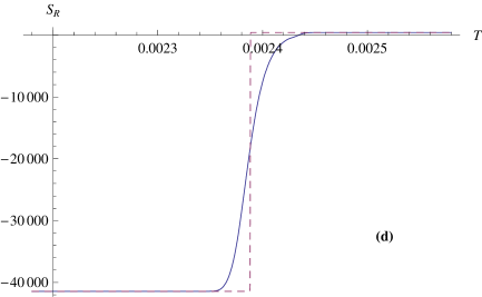
Figure 4: Typical behavior of $S_{R}$ vs. $T$ calculated from RZ (continuous line) and TA (dashed line), for $L=200$, temperatures close to $T_{c}$ and different values of $N$: (a) $N=10^{-80}$, (b) $N=10^{-100}$, (c) $N=10^{-130}$, (d) $N=10^{-180}$. The convergence of RZ to TA when $N$ decreases is displayed.

4.3 Latent heat

From the expressions for the entropy, we calculate the regular latent heat of the transition:

$$l_{R}\left(L,N,T=T_{c}\right)=T_{c}\Delta S_{R}(T_{c})=T_{c}\{S_{R}(T>T_{c})-S_{R}(T<T_{c})\}=[L/2]\epsilon\ .$$ (4.5)

Eq. (4.5) shows that the phase transition in the model we have considered is of first order [30]. Note that (4.5) does not depend on $N$: this result could be expected, since the latent heat is the energy released or absorbed by the system during the transition, and $N$ is associated with the concentration of Mg⁺⁺, and, therefore, plays the effective role of an external variable regardless of the way in which it has been introduced. Eq. (4.5) expresses that the energy exchange between the system and the bath during the phase transition is $[L/2]\epsilon$, since there are $[L/2]$ parings between pairs of bases, which could be created or broken during the transition, depending on the direction in which $T$ crosses $T_{c}$.

5 Conclusions

In this paper we have studied, using both analytical and numerical methods, the $T-$dependent phase transition in a simplified model of the RNA molecule, in the regime of large concentration of positive ions in solution. This regime has similarities with the large density phase of polymers studied by de Gennes. We have presented an analytical expression for the critical temperature $T_{c}$, which tends to zero in the thermodynamic limit. The critical temperature separates the only configuration without interaction between the bases (and, therefore, of genus zero) which is dominant for $T<T_{c}$, from the configurations with high energy and large genera equal to $[L/4]$, which dominate for $T>T_{c}$. This transition is no to be confused with the coil-globule transition, which appears for low concentration of positive ions in solution. Due to the interesting dependence of the genus with the temperature, we call this a topological phase transition, and we have shown that the transition is of first order. Although the model studied is very simple, we are confident that most of the properties studied here might be robust and extend to more realistic ones, given the importance of the saturation property of the elementary base interaction, that this model preserves.

Acknowledgments

MdE thanks M. M. Reynoso for discussions.

References

- [1] I. Tinoco Jr. and C. Bustamante, J. Mol. Biol. 293 (1999) 271.
- [2] H. Orland, A. Zee, Nucl. Phys. B 620 (2002) 456.
- [3] M. M ller, Phys. Rev. E 67 (2003) 021914.
- [4] C. Hyeon, R. I. Dima, and D. Thirumalai, J. Chem. Phys. 125 (2006) 194905.
- [5] V. S. Pande, A. Yu. Grosberg, and T. Tanaka, Rev. Mod. Phys. 72 (2000) 259.
- [6] G. Vernizzi, H. Orland, A. Zee, Phys. Rev. Lett. 94 (2005) 168103.
- [7] G. Vernizzi, H. Orland, Acta Phys. Pol. 36 (2005) 2821.
- [8] M. G. dell’Erba, G. R. Zemba, Phys. Rev. E 79 (2009) 011913.
- [9] M. Pillsbury, J. A. Taylor, H. Orland, A. Zee, Phys. Rev. E 72 (2005) 011911.
- [10] T. Lindahl, A. Adams, J. R. Fresco, PNAS 55 (1966) 941.
- [11] R. F. Gesteland, T. R. Cech, J. F. Atkins (Eds.), Chapter 12, The RNA World, Second Edition, Monograph Series 37, Cold Spring Harbor Laboratory Press (1999).
- [12] V. K. Misra, D. E. Draper, PNAS 98 (2001) 12456.
- [13] D. E. Draper, RNA 10 (2004) 335.
- [14] K. J. Travers, N. Boyd, D. Herschlag, RNA 13 (2007) 1205.
- [15] E. V. Hackl, Y. P. Blagoi, Acta Bioch. Pol. 47 (2000) 103.
- [16] G. ’t Hooft, Nucl. Phys. B 72 (1974) 461.
- [17] P. -G. de Gennes, Scaling Concepts in Polymer Physics, Cornell Univ. Press, Ithaca (New York), (1979).
- [18] G. Vernizzi, P. Ribeca, H. Orland, A. Zee, Phys. Rev. E 73 (2006) 031902.
- [19] H. Noguchi, K. Yoshikawa, Chem. Phys. Lett. 278 (1997) 184.
- [20] M. Ueda, K. Yoshikawa, Phys. Rev. Lett. 77 (1996) 2133.
- [21] S. Doniach, T. Garel, H. Orland, J. Chem. Phys. 105 (1996) 1601.
- [22] I. Garg, N. Deo, http://arXiv.org/abs/0802.2440v2.
- [23] I. Garg, N. Deo, http://arXiv.org/abs/0809.1016v1.
- [24] I. S. Gradshteyn, I. M. Ryzhik, A. Jeffrey, D. Zwillinger,Table of Integrals, Series, and Products, Fifth Edition, Academic Press, New York (1994).
- [25] M. ivkovi, Ser. Mat. Fiz. 498-541 (1975) 217-221.
- [26] M. Abramowitz, I. A. Stegun, Handbook of Mathematical Functions, Ninth Printing, Dover Publications, NY (1972).
- [27] S. Wolfram, Mathematica, Addison-Wesley, New York (1991).
- [28] S. Doniach, T. Garel, H. Orland, J. Chem. Phys. 105 22.
- [29] T. Gluick, R. Gerstner, D. Draper, J. Mol. Biol. 270 (1997) 451.
- [30] H. E. Stanley, Introduction to Phase Transitions and Critical Phenomena, Oxford Science Publications, New York (1971).