Coherent potential approximation for spatially correlated disorder

Abstract

The coherent-potential approximation (CPA) is extended to describe satisfactorily the motion of particles in a random potential which is spatially correlated and smoothly varying. In contrast to existing cluster-CPA methods, the present scheme preserves the simplicity of the conventional CPA but leads to a momentum and frequency-dependent self-energy. Its accuracy is checked by a comparison with the exact moments of the Green’s function, and with the spectral function from numerical simulations. The scheme is applied to excitonic absorption spectra in different spatial dimensions.

I Introduction

Disorder is a pertinent feature in many solid state systems, and has been a topic of interest and intense research for many decades. The prototype system is a binary alloy where the chemical constituents are randomly (and spatially uncorrelated) placed on the sites of a regular lattice. Adding next neighbor hopping for the electronic band under consideration, and leaving out any additional interactions, we are left with the discrete Anderson model which has been widely studied, mostly in view of calculating the electronic density of states.

A break through in the theoretical treatment was the invention of the coherent-potential approximation (CPA), initially proposed by Soven Soven and further developed by Velicky, Kirkpatrick, and Ehrenreich VKE ; Velicky . In a nutshell, the system is replaced by a perfect crystal (effective medium) with a complex self energy instead of the disorder potential, whose value is fixed by demanding that the electron at the central site is not scattered off the surrounding medium (on the average). The standard (single-site) version of the CPA is characterized by a momentum-independent self energy, and leaves out finer details in the density of states. It has been extended by embedding not only a single site but a larger cluster into the effective medium. Consequently, in this embedded cluster CPA Cluster , a self-energy matrix instead of a single element has to be determined self-consistently. This can work satisfactorily for one spatial dimension Eggarter , but apart from increasing the numerical work, it is prone to numerical instabilities and shows sometimes an incorrect analytic behavior. Such problems have been reported by Mills and co-workers Mills when introducing the ”travelling cluster method” for the bulk case.

Not unexpected, a single-site approximation will fail completely if already the underlying disorder has a spatial correlation. This happens for an alloy with clustering in the chemical composition. For bulk semiconductor material with impurities, the finite range of the impurity potential itself gives rise to a spatial correlation, independent on the placement of the impurity atoms. Among the papers which have applied and refined cluster-CPA methods for correlated disorder, we quote Ref. Mookerjee where further references on earlier work can be found. Systematic improvements have been achieved by Jarrell applying his dynamical cluster approximation (DCA) to disorder problems Jarrell . This approach has been later adopted to correlated disorder as well Maier . However, in order to preserve the correct analytic properties in the DCA, the momentum dependence of the self-energy had to be coarse grained according to the cluster size used (see the critical discussion of Rowlands Rowlands ). A cluster CPA with only one complex function of frequency to be determined self-consistently has been derived recently in Ref. Laad , but was applied to next-neighbor correlations only.

Our main motivation to deal with correlated disorder came from excitons (Coulomb-bound electron-hole pairs) where the averaging with the ground-state wave function produces a correlated potential quite naturally. The reader who is not so much interested in exciton physics may skip the corresponding Sec. II and proceed immediately with the formulation of the problem in terms of the continuous Anderson model (Sec. III). The coherent-potential approximation is extended to a (smoothly) correlated potential landscape in Sec. IV, introducing a momentum and frequency-dependent self-energy. The resulting scheme preserves the simplicity of the standard CPA in so far as for each momentum and frequency, a single root searching in the complex plane is sufficient. In Sec. V, the exact moments of the spectral function are compared with those of the correlated CPA. Numerical results for the spectral function are presented in Sec. VI and compared to numerically exact simulation results. For the latter, the Kernel polynomial method (KPM) Alvermann is applied which rests upon an expansion of the Hamiltonian into Chebyshev polynomials. In Appendix A it is shown that the present method guarantees the proper analytic behavior (Herglotz properties) of the self-energy in the complex-frequency plane. Explicit expressions for several functions needed in the correlated CPA are listed in the Appendix B while in Appendix C results for the exact moments are collected.

II Application: Excitons in disordered semiconductors

Pioneering work on excitons and disorder has been done by Baranovskii and Efros Baranovski emphasizing the distinct role of the relative motion of electron and hole within the exciton in contrast to the center-of-mass (cm) motion of the exciton as a whole. Both motions average over the underlying disorder and lead to a double-step ”motional narrowing” which gives rise to an inhomogeneous exciton line width well below the width of the band-edge fluctuations. In the first (relative motion) step one needs a proper definition of the ”excitonic volume” which is related to the integral over the fourth power of the relative wave function Zim89 ; LeeBajaj . This has been refined later to take into account the magnetic-field dependence of the relative exciton motion Lyo . The implementation of the second (cm motion) step was more complicated. An early attempt Kanehisa was using a CPA-like treatment of electrons and holes separately but has decoupled the formation of excitons from the disorder influence following Ref. Velicky .

If the exciton is well localized on a single lattice site (Frenkel exciton), only the cm motion has to be considered. This is the realm of excitations in tight-binding chains where disorder treatments have a long history. An early comparison between simulation and CPA for uncorrelated potentials has been presented by Huber and Ching Huber . The corresponding motional narrowing has been discussed widely based on simulations Reineker . Correlated disorder of a very specific form (dimers of identical energy) has been treated in Ref. Adame via numerical averaging over disorder realizations. In Ref. Bakalis , Frenkel excitons in silver-halide systems have been investigated using the standard CPA. Assuming still uncorrelated disorder, the model has been generalized to potential distributions more complicated than simple Gaussian.

In the case of moderate disorder (the inhomogeneous exciton line width being small compared with its binding energy), the ground-state exciton wave function for relative motion may be treated as unaffected by disorder. Then, the task reduces to solve an effective one-particle problem for the cm motion. Still, the relative motion was reducing the fluctuations of the effective cm potential (first step motional narrowing). However, much more important is that the resulting cm potential is now spatially correlated at least over distances comparable to the exciton Bohr radius – even if the underlying band-edge fluctuations were not correlated at all. This was our main stimulus to treat the exciton cm motion in a correlated potential.

A straightforward way to do so are numerical simulations: For a given potential, the Schrödinger equation is solved for eigenvalues and eigenfunctions, wherefrom the spectral function can be extracted easily. Note that at zero cm momentum, the spectral function agrees with the absorption line shape of the inhomogeneously broadened exciton. A lot more effective is to solve the time-dependent Schrödinger equation for the Green’s function which gives upon time Fourier transformation the spectral function directly Huber ; GlutschTime . Mandatory, however, is the subsequent average over many disorder realizations in order to get a reasonably smooth line shape. This can be an expensive task limited by both computing time and memory resources. Therefore, it is compelling to look for a scheme such as CPA which avoids large scale computations but the CPA needs to be adapted to spatial correlation as done in the present paper.

For excitons in a mixed semiconductor crystal, the basic random quantity $U({\bf r})$ is the local energy gap due to $A$ and $B$ atoms placed uncorrelated on the lattice sites (see Eq. (6)). In this case, the smoothing function $W({\bf r})$ is determined by the exciton relative wave function. Assuming for the 1s ground-state exciton the standard exponential expression, we have

$$W({\bf r})\propto\sigma e^{-r/\xi}$$ (1)

where the potential correlation length $\xi$ is proportional to the exciton Bohr radius $a_{B}$. In semiconductor nanostructures as quantum wells (quantum wires), an additional source of disorder is the fluctuation of the well width (the wire cross section), which leads to a variation of the confinement energies. If the length scale of these fluctuations is smaller than the exciton Bohr radius, it can be approximated again as a delta-correlated random process $U({\bf r})$. The smoothing function $W({\bf r})$ is then the appropriate relative exciton wave function in lower dimensions.

In the case of electrons moving in the potential of densely spaced randomly distributed impurities, $W({\bf r})$ is proportional to the (screened) potential of a single impurity. In Appendix A, we give explicit expressions for exponential and for Gaussian type of the potential correlation, and are listing more details taken from Ref. TakaRev .

A more sophisticated disorder-related effect is quantum-mechanical level repulsion of excitons which can be seen in time-resolved Rayleigh scattering SavonaZim or spectral correlation spectroscopy Lienau . While these effects are of two-particle nature we concentrate in the present paper on the one-particle level which is sufficient to describe the absorption line shape of excitons. For a review on our work on excitons and disorder in nanostructures see Refs. TakaRev ; RungeSSP . Quite recently, we were able to do simulations for optical spectra without the separation into relative and cm exciton motion Grochol .

III Formulation of the problem

Let us consider a single particle (electron, exciton,…) with mass $M$ which moves in a random potential $V({\bf r})$. The one-particle Green’s function obeys the inhomogeneous Schrödinger equation

$$\left(-\frac{\hbar^{2}}{2M}\Delta_{{\bf r}}+V({\bf r})-\hbar z\right){\cal G}({\bf r},{\bf r}^{\prime},z)=-\delta({\bf r}-{\bf r}^{\prime})\,,$$ (2)

with the complex energy $\hbar z$. This problem is usually called Continuous Anderson model. The one-particle density of states is defined as

$$\rho(\omega)=\frac{1}{\Omega}\left\langle\int d{\bf r}\,\mbox{\sl Im\,}{\cal G}({\bf r},{\bf r},\omega-i0)\right\rangle\,.$$ (3)

Further, we are interested in the spectral function $A_{\bf k}(\omega)$

$$A_{\bf k}(\omega)=\frac{1}{\Omega}\left\langle\int d{\bf r}\,d{\bf r}^{\prime}\,e^{i{\bf k}({\bf r}-{\bf r}^{\prime})}\mbox{\sl Im\,}{\cal G}({\bf r},{\bf r}^{\prime},\omega-i0)\right\rangle\,.$$ (4)

($\Omega$ is a normalization volume). For excitons, ${\bf r}$ has to be understood as the center-of-mass coordinate, and the appropriate mass is $M=m_{e}+m_{h}$. The line shape of the excitonic absorption (into the 1s ground state) is given by the spectral function at ${\bf k}={\bf k}_{light}\approx 0$.

The angular brackets in Eqs. (3 and 4) represent the average over all realizations of the random potential $V({\bf r})$. We take the average potential as zero of energy (that is the band edge of the virtual crystal). Therefore, the disorder potential has zero mean value. Further, we assume it to be Gauss distributed with variance $\sigma$, and define its spatial correlation via

$$\langle V({\bf r})\rangle=0\,,\quad\langle V({\bf r})\,V({\bf r}^{\prime})\rangle=\sigma^{2}\,g({\bf r}-{\bf r}^{\prime})\,.$$ (5)

The correlation function $g({\bf r})$ is therefore normalized to $g({\bf r}=0)=1$. All higher order correlations are assumed to factorize. Such type of potentials can be generated by integrating with a smoothing function $W({\bf r})$ over a delta-correlated basic random process $U({\bf r})$

$$V({\bf r}) = \int d{\bf r}^{\prime}\,W({\bf r}-{\bf r}^{\prime})\,U({\bf r}^{\prime})\,,$$ (6)

$$\langle U({\bf r})\,U({\bf r}^{\prime})\rangle = \delta({\bf r}-{\bf r}^{\prime})\,.$$

The correlation function is related to $W$ via the convolution

$$\sigma^{2}g({\bf r})=\int d{\bf r}^{\prime}\,W({\bf r}+{\bf r}^{\prime})\,W({\bf r}^{\prime})\,.$$ (7)

Let $W({\bf r})$ decay on the scale $\xi$. Then, the resulting random potential varies smoothly over distances of order $\xi$, and the correlation of the potential can be quantified by the kinetic energy on the length scale $\xi$

$$E_{c}=\frac{\hbar^{2}\xi^{-2}}{2M}\,.$$ (8)

Obviously, there are only two energies in the theory: The correlation energy $E_{c}$, and the disorder strength $\sigma$. One of them can be taken as energy scale. Given a certain type of correlation (exponential or Gaussian), the spectral function (or exciton line shape) depends therefore only on the single parameter $E_{c}/\sigma$.

IV Correlated CPA

The basic idea of the CPA is sketched as follows Soven ; VKE : The entire space is divided into a central cluster where the disorder average has to be performed exactly, and into the remaining outer part which is described as an effective medium with averaged (but complex) potential, respectively, self-energy $\Sigma(z)$. For the determination of $\Sigma(z)$, the Green’s function of the effective medium $G(z)$ is put equal to the cluster average of the full Green’s function (cluster embedded into the effective medium). In the conventional CPA, the central cluster is reduced to a single site, and the self-consistency condition for $\Sigma(z)$ can be formulated as a vanishing of the averaged $t$-matrix (Soven’s equation, Soven ). In a correlated potential, the abrupt change between the on-site potential $V({\bf r}=0)$ and the self-energy $\Sigma(z)$ outside is in contrast to the smooth behavior of any potential realization. Choosing a larger cluster is expected to improve, but – apart from analyticity problems encountered – the abrupt change at the cluster boundary remains unaffected. In order to illustrate this point we look for the conditional probability to find a potential value $V_{1}$ at a distance ${\bf r}$ keeping $V_{0}\equiv V({\bf r}=0)$ fixed:

$$P(V_{1},{\bf r}|V_{0})=\frac{1}{\sqrt{2\pi}\sigma_{1}({\bf r})}\exp\left(-\frac{(V_{1}-V_{0}g({\bf r}))^{2}}{2\sigma_{1}^{2}({\bf r})}\right)\,.$$ (9)

The most probable value of $V_{1}=V({\bf r})$ is therefore given by

$$\left.V({\bf r})\right|_{prob.}=V_{0}\,g({\bf r})\,,$$ (10)

and distributed with a variance $\sigma_{1}^{2}({\bf r})=\sigma^{2}(1-g^{2}({\bf r}))$ increasing with distance towards $\sigma$ (see Fig. 1 for a visualization). The main idea of the present CPA extension is to use a smooth interpolation between the central ”most probable” potential shape and the effective medium outside which is assumed to have a nonlocal self-energy,

$$V({\bf r})\Rightarrow V_{0}\,g({\bf r})\,\delta({\bf r}-{\bf r}^{\prime})+\Sigma({\bf r}-{\bf r}^{\prime},z)(1-g({\bf r}^{\prime}))\,.$$ (11)

In this way, any sharp break is avoided, and the effective Schrödinger equation reads

$$\left(-\frac{\hbar^{2}}{2m}\Delta_{{\bf r}}+V_{0}g({\bf r})-\hbar z\right){\cal G}({\bf r},{\bf r}^{\prime\prime},z) +$$ (12)

$$\int d{\bf r}^{\prime}\,\Sigma({\bf r}-{\bf r}^{\prime},z)\left(1-g({\bf r}^{\prime})\right){\cal G}({\bf r}^{\prime},{\bf r}^{\prime\prime},z) = -\delta({\bf r}-{\bf r}^{\prime\prime})\,.$$

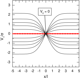
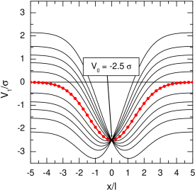
Figure 1: (color online) Probability distribution of the Gauss correlated potential around a fixed potential value at $x=0$ (top: $V_{0}=0$, bottom: $V_{0}=-2.5\,\sigma$). The curve with dots marks the most probable value $V_{0}\,g(x)$. Other lines refer to probabilities 0.9, 0.7, 0.5, 0.3, 0.1 relative to the maximum (at each $x$ value).

Fourier transformation into reciprocal space yields

$$(\epsilon_{\bf k}+\Sigma_{{\bf k}}(z)-\hbar z)\,{\cal G}_{{\bf k}{\bf k}^{\prime}}(z) +$$ (13)

$$+\,(V_{0}-\Sigma_{{\bf k}}(z))\sum_{\tilde{\bf k}}g_{{\bf k}\tilde{\bf k}}\,{\cal G}_{\tilde{\bf k}{\bf k}^{\prime}}(z) = -\delta_{{\bf k}{\bf k}^{\prime}}\,,$$

with dispersion $\epsilon_{\bf k}=\hbar^{2}k^{2}/2M$. The Fourier transform of the potential correlation function, $g_{\bf k}$, can be expressed via the smoothing function as

$$\sigma^{2}g_{\bf k}=\left|W_{\bf k}\right|^{2}\;,\quad W_{\bf k}=\frac{1}{\sqrt{\Omega}}\int d{\bf r}\,e^{-i{\bf k}{\bf r}}\,W({\bf r})\,.$$ (14)

The normalization $g(0)=1$ transforms into $\sum_{\bf k}g_{{\bf k}}=1$. Eq. (13) can be written as

$${\cal G}_{{\bf k}{\bf k}^{\prime}}(z)=G_{\bf k}(z)\left[\delta_{{\bf k}{\bf k}^{\prime}}+(V_{0}-\Sigma_{{\bf k}}(z))\sum_{\tilde{\bf k}}g_{{\bf k}\tilde{\bf k}}\,{\cal G}_{\tilde{\bf k}{\bf k}^{\prime}}(z)\right]$$ (15)

introducing the Green’s function of the effective medium

$$G_{{\bf k}}(z)=\frac{1}{\hbar z-\epsilon_{\bf k}-\Sigma_{{\bf k}}(z)}$$ (16)

which is diagonal in momentum space. In contrast, the Green’s function Eq. (15) is nondiagonal since we have located the central potential $V_{0}$ at ${\bf r}=0$ which has spoiled the translational invariance. Placing $V_{0}$ at position ${\bf r}_{0}$ leads simply to the Green’s function ${\cal G}({\bf r}-{\bf r}_{0},{\bf r}^{\prime}-{\bf r}_{0},z;V_{0})$ (for clarity, we have marked the dependence on $V_{0}$). Therefore, the embedding into the effective medium should contain two steps: (i) an integration over ${\bf r}_{0}$ and (ii) an average over the (Gaussian) distribution of the central potential

$$P(V_{0})=\frac{1}{\sqrt{2\pi}\sigma}e^{-V_{0}^{2}/2\sigma^{2}}\,.$$ (17)

The self-consistency condition in the spirit of the CPA reads therefore

$$G({\bf r}-{\bf r}^{\prime},z)=\frac{1}{\Omega}\int\!d{\bf r}_{0}\int\!dV_{0}P(V_{0}){\cal G}({\bf r}-{\bf r}_{0},{\bf r}^{\prime}-{\bf r}_{0},z;V_{0})$$ (18)

or after Fourier transformation

$$\left\langle{\cal G}_{{\bf k}{\bf k}}(z;V_{0})\right\rangle_{V_{0}}=G_{{\bf k}}(z)\,.$$ (19)

Note that only the diagonal elements of ${\cal G}_{{\bf k}{\bf k}^{\prime}}(z)$ enter the CPA condition.

In order to avoid the solution of the matrix equation Eq. (15) we specify our Ansatz further by factorizing the momentum dependence as

$${\cal G}_{{\bf k}{\bf k}^{\prime}}(z;V_{0})\Rightarrow G_{\bf k}(z)\,H_{{\bf k}^{\prime}}(z;V_{0})\,.$$ (20)

Then, Eq. (15) at ${\bf k}={\bf k}^{\prime}$ can be solved immediately, and the self-consistency condition Eq. (19) converts into $\langle H_{{\bf k}}(z;V_{0})\rangle_{V_{0}}=1$. Explicitly, we have

$$\left\langle\frac{1}{1-(V_{0}-\Sigma_{{\bf k}}(z))R_{\bf k}(\hbar z;\{\Sigma\})}\right\rangle_{V_{0}}=1$$ (21)

with the auxiliary function

$$R_{\bf k}(\hbar z;\{\Sigma\})=\sum_{{\bf k}^{\prime}}g_{{\bf k}-{\bf k}^{\prime}}G_{{\bf k}^{\prime}}(z)=\sum_{{\bf k}^{\prime}}\frac{g_{{\bf k}-{\bf k}^{\prime}}}{\hbar z-\epsilon_{{\bf k}^{\prime}}-\Sigma_{{\bf k}^{\prime}}(z)}\,.$$ (22)

The argument for chosing the present Ansatz Eqs.(11,20) was to exactly reproduce three well-known limiting cases:

(i) White noise: For an uncorrelated potential ($g_{{\bf k}}=const.$), the auxiliary function Eq. (22) and therefore the self-energy do not depend on momentum. Thus, the conventional CPA is fully recovered which reads VKE

$$\left\langle\frac{1}{1-(V_{0}-\Sigma(z))\frac{1}{\cal N}\sum_{{\bf k}}\frac{1}{\hbar z-\epsilon_{\bf k}-\Sigma(z)}}\right\rangle_{V_{0}}=1\,.$$ (23)

Here, a finite band width has to be implemented by restricting the sum over ${\bf k}$ to the first Brillouin zone, having ${\cal N}$ discrete momentum points. The parabolic dispersion $\epsilon_{\bf k}$ must be replaced by a tight-binding expression, and one arrives at the CPA of the discrete Anderson model with site disorder.

(ii) Classical limit: If the correlation has infinite range, we have $g({\bf r})=1$ ($g_{{\bf k}-{\bf k}^{\prime}}=\delta_{{\bf k}{\bf k}^{\prime}}$), and the solution of Eq. (21) is simply

$$\left\langle\frac{\hbar z-\epsilon_{\bf k}-\Sigma_{{\bf k}}(z)}{\hbar z-\epsilon_{\bf k}-V_{0}}\right\rangle_{V_{0}}=1$$ (24)

with the result

$$G_{{\bf k}}(z)=\left\langle\frac{1}{\hbar z-\epsilon_{\bf k}-V_{0}}\right\rangle_{V_{0}}\,.$$ (25)

The Green’s function mirrors the potential distribution displaced by $\epsilon_{\bf k}$ as expected in this case.

(iii) Second Born approximation: For weak coupling, Eq. (21) can be expanded into a geometrical series

$$\sum_{j=0}^{\infty}\left\langle\left(V_{0}-\Sigma_{\bf k}(z)\right)^{j}\right\rangle_{V_{0}}R^{j}_{\bf k}(\hbar z;\{\Sigma\})=1\,.$$ (26)

Up to second order ($j\leq 2$), we need the disorder averages $\langle V_{0}\rangle=0$ and $\langle V_{0}^{2}\rangle=\sigma^{2}$. This results in leading order to the self-energy

$$\Sigma^{2B}_{{\bf k}}(z)=\sigma^{2}R_{\bf k}(\hbar z;\{\Sigma^{2B}\})\equiv\sum_{{\bf k}^{\prime}}\frac{\sigma^{2}\,g_{{\bf k}-{\bf k}^{\prime}}}{\hbar z-\epsilon_{{\bf k}^{\prime}}-\Sigma^{2B}_{{\bf k}^{\prime}}(z)}$$ (27)

which is just the self-consistent second Born approximation, also called ”random coupling method” Kraich . This agreement was the guiding principle for selecting the appropriate ”switch on” of the self-energy in Eq. (11). We were starting with $V_{0}g({\bf r})\delta({\bf r}-{\bf r}^{\prime})+\Sigma({\bf r}-{\bf r}^{\prime},z)(1-\hat{g}({\bf r}^{\prime}))$ with a yet unspecified function $\hat{g}({\bf r}^{\prime})$. Consequently, a second auxiliary function $\hat{R}$ appears as factor to the (explicit) self-energy in Eq. (21) and Eq. (26), while $V_{0}$ stays with the original $R$ ($\hat{R}$ is defined like Eq. (22) but contains $\hat{g}_{\bf k}$ instead of $g_{\bf k}$). In second Born quality, the self-energy reads now $\Sigma^{2B}=\sigma^{2}R^{2}/\hat{R}$ (with arguments suppressed). The comparison with Eq. (27) dictates $\hat{R}\equiv R$ that is $\hat{g}\equiv g$, which justifies a posteriori the choice made in Eq. (11).

An application of the self-consistent second Born approximation to excitons in disordered semiconductors can be found in Ref. Stroucken . In diagram language, this self-energy consists of the simplest diagram where the averaged Green’s function appears just once. Although being an approximation with inferior quality (see Sec. VI), already here a self-energy comes out which depends continuously on momentum (the frequency $z$ plays the role of a parameter). Other approaches like Jarrell’s DCA Maier – while much more sophisticated with respect to local correlations – fail to reproduce the self-consistent second Born approximation in the appropriate limit, coming up with a discontinuous momentum dependence of the self-energy.

The coupling of self-energies at different ${\bf k}$ points in Eqs. (21 and (22) complicates the numerics since the self-consistency can be achieved only iteratively. Replacing $\Sigma_{{\bf k}^{\prime}}(z)$ by $\Sigma_{{\bf k}}(z)$ in Eq. (22) reduces the problem to a simple root-searching task in the complex plane for the single quantity $\Sigma_{{\bf k}}(z)$ (at given values of ${\bf k}$ and $z$)

$$\left\langle\frac{1}{1-(V_{0}-\Sigma_{{\bf k}}(z))R_{\bf k}(\hbar z-\Sigma_{{\bf k}}(z))}\right\rangle_{V_{0}}=1$$ (28)

with the auxiliary function now written as

$$R_{\bf k}(\hbar z)=\sum_{{\bf k}^{\prime}}\frac{g_{{\bf k}-{\bf k}^{\prime}}}{\hbar z-\epsilon_{{\bf k}^{\prime}}}\,.$$ (29)

We call this diagonal coherent-potential approximation and show in Sec. V that the agreement with the simulation results is not much sacrificed. With the self-consistently determined self-energy, the spectral function is obtained as

$$A_{\bf k}(\omega)=\left.\mbox{\sl Im\,}\frac{1}{\hbar z-\epsilon_{\bf k}-\Sigma_{{\bf k}}(z)}\,\right|_{z=\omega-i0}$$ (30)

and the density of states can be calculated via

$$\rho(\omega)=\frac{1}{\Omega}\sum_{\bf k}A_{\bf k}(\omega)\,.$$ (31)

V Analysis of moments

Before presenting numerical results, it is useful to provide a somewhat deeper insight into the quality of the CPA method presented here. We focus on the moments of the spectral function defined as

$$M_{n}({\bf k})=\int\frac{d\hbar\omega}{\pi}A_{\bf k}(\omega)\left(\hbar\omega-\epsilon_{\bf k}\right)^{n}\,.$$ (32)

As a benchmark, we are going to check the moments in CPA against the exact ones. The first moments describe some basic features of the spectral function: $M_{0}=1$ gives the normalization, $M_{1}$ is the average position with respect to the bare dispersion $\epsilon_{\bf k}$, and $M_{2}$ is the overall width. More subtle is the effect of the next moments, where $M_{3}$ can be related to the asymmetry (or skewness), and $M_{4}$ to the importance of tails. A distinct advantage is that the moments can be evaluated exactly – as long as they are finite (see Appendix B). The clue is the spectral representation of the (disorder-averaged) Green’s function

$$G_{\bf k}(z)=\int\frac{d\hbar\omega}{\pi}\frac{A_{\bf k}(\omega)}{\hbar z-\hbar\omega}$$ (33)

which leads to the asymptotic expansion

$$G_{\bf k}(z)\simeq\sum_{n=0}^{\infty}\frac{M_{n}({\bf k})}{\left(\hbar z-\epsilon_{\bf k}\right)^{n+1}}$$ (34)

for $|z|\rightarrow\infty$. The exact operator expression

$$G_{\bf k}(z)=\langle{\bf k}|\left(\hbar z-{\cal H}\right)^{-1}|{\bf k}\rangle$$ (35)

can be expanded in a similar way, and the moments are found as disorder averages of powers of the Hamiltonian in Eq. (2)

$$M_{n}({\bf k})=\langle{\bf k}|\left({\cal H}-\epsilon_{\bf k}\right)^{n}|{\bf k}\rangle\,.$$ (36)

For the evaluation, it is useful to work in reciprocal space with

$$\langle{\bf k}|{\cal H}|{\bf k}^{\prime}\rangle=\epsilon_{\bf k}\delta_{{\bf k}{\bf k}^{\prime}}\,+\,V_{{\bf k}-{\bf k}^{\prime}}\,,$$ (37)

where $V_{\bf q}$ is the potential of a single realization in Fourier space. The first steps give immediately

$$M_{0}=1\;,\quad M_{1}=\langle V_{{\bf k}-{\bf k}}\rangle=0\,,$$ (38)

since averages over odd powers of the potential vanish. In the next step

$$M_{2}=\sum_{{\bf k}^{\prime}}\langle V_{{\bf k}-{\bf k}^{\prime}}\,V_{{\bf k}^{\prime}-{\bf k}}\rangle=\sigma^{2}$$ (39)

holds, using $\langle V_{{\bf q}}\,V_{-{\bf q}^{\prime}}\rangle=\sigma^{2}\delta_{{\bf q}{\bf q}^{\prime}}g_{\bf q}$ and the normalization of the potential correlation. Interestingly enough, the first three moments are universal, i.e. they do not depend on the correlation energy, and have no ${\bf k}$ dependence either. In higher orders, a mixing between kinetic energy and potential correlation appears, which can be quantified by

$$K_{n}({\bf k})=\sum_{{\bf k}^{\prime}}g_{{\bf k}-{\bf k}^{\prime}}\left(\epsilon_{{\bf k}^{\prime}}-\epsilon_{\bf k}\right)^{n}\,.$$ (40)

For the third moment, we obtain

$$M_{3}=\sigma^{2}K_{1}$$ (41)

which is again independent on momentum due to the mirror symmetry $g_{\bf q}=g_{-{\bf q}}$. In the next order

$$M_{4}({\bf k})=\sigma^{2}K_{2}({\bf k})\,+\,3\sigma^{4}\,,$$ (42)

where the second term stems from the average over four potentials, $\langle V^{4}({\bf r})\rangle=3\sigma^{4}$. We proceed up to the fifth moment

$$M_{5}({\bf k})=\sigma^{2}K_{3}({\bf k})\,+\,10\sigma^{4}K_{1}\,.$$ (43)

Explicit expressions for different correlation type and dimensionality are collected in Appendix C.

At still larger $n$, things are getting involved rapidly. By dimensional arguments, $K_{n}({\bf k}=0)\propto E_{c}^{n}$ and the moments at ${\bf k}=0$ have the following structure

$$M_{n}(0)=\sum_{j=1}^{[n/2]}a_{n,j}\,\sigma^{2j}\,E_{c}^{n-2j}$$ (44)

which shows up already in the first moments listed above. Only the leading $\sigma$ power has a simple structure, namely $a_{n,j=n/2}=1\cdot 3\cdots(n-3)\cdot(n-1)$ for even $n$. Taken alone, these terms would reconstruct just the Gaussian potential distribution (classical limit). Our earlier work using the derivation of moments is summarized in Ref.  RungeSSP . The exact coefficients $a_{n,j}$ and thus the moments have been generated using symbolic manipulations. However, the numerical load increases exponentially and we were restricted to $n\leq 20$. On the other hand, the numerical results gave clear evidence that much more moments (of the order of thousands) are needed for a proper description of the spectral function. Consequently, earlier attempts to work with an infinite (but restricted) subset were not successful GlutschMom . In particular at large $E_{c}/\sigma$, even negative portions of the spectral function may appear.

To complete the comparison, we are now evaluating the moments in CPA. First, the general relation between moments of the spectral function and of the self-energy is established. In analogy to Eq. (34), the self-energy moments $S_{l}({\bf k})$ are defined by

$$\Sigma_{{\bf k}}(z)\simeq\sum_{l=0}^{\infty}\frac{S_{l}({\bf k})}{\left(\hbar z-\epsilon_{\bf k}\right)^{l+1}}\,.$$ (45)

We have no constant term in this expansion since the band edge of the virtual crystal was taken as zero of energy. Inserting Eq. (45) into Eq. (16) gives together with Eq. (34)

$$M_{0}=1\,,\quad M_{1}=0\,,\quad M_{n}({\bf k})=\sum_{l=0}^{n-2}S_{l}({\bf k})\,M_{n-l-2}({\bf k})\,.$$ (46)

A similar recursion relation between moments holds for the electron gas Vogt – with Coulomb interaction instead of disorder. The auxiliary function Eq. (29) decays at least as $1/E$ where $E\equiv\hbar z-\epsilon_{\bf k}$ in the following. Keeping terms up to $E^{-5}$, we restrict the expansion Eq. (26) of the defining CPA equation Eq. (28) to $j\leq 5$ and perform the disorder average over the ”central” potential $V_{0}$ using

$$\langle V_{0}^{2}\rangle=\sigma^{2}\,,\quad\langle V_{0}^{4}\rangle=3\sigma^{4}$$ (47)

(odd orders do vanish). After division with $R$ we arrive at

$$\Sigma=\left(\sigma^{2}+\Sigma^{2}\right)R-3\sigma^{2}\Sigma R^{2}+3\sigma^{4}R^{3}$$ (48)

which is accurate up to $E^{-4}$. Therefore, thanks to Eq. (46), we can obtain the spectral moments up to $M_{5}$ as desired. In a next step, we write the auxiliary function needed in Eq. (28) as

$$R_{\bf k}(\hbar z-\Sigma_{{\bf k}}(z))=\frac{1}{E}\sum_{{\bf k}^{\prime}}\frac{g_{{\bf k}-{\bf k}^{\prime}}}{1-(\epsilon_{{\bf k}^{\prime}}-\epsilon_{\bf k}+\Sigma_{{\bf k}}(z))/E}$$ (49)

and expand this up to $1/E^{4}$

$$R_{\bf k}=\frac{1}{E}+\frac{K_{1}}{E^{2}}+\frac{\sigma^{2}+K_{2}({\bf k})}{E^{3}}+\frac{3\sigma^{2}K_{1}+K_{3}({\bf k})}{E^{4}}\,.$$ (50)

Now we are ready to equate powers of $E^{-n}$ in Eq. (48) iteratively. In successive steps using Eq. (50) we obtain

$$S_{0}({\bf k}) = \sigma^{2}$$

$$S_{1}({\bf k}) = \sigma^{2}K_{1}$$ (51)

$$S_{2}({\bf k}) = \sigma^{2}K_{2}({\bf k})+\,2\sigma^{4}$$

$$S_{3}({\bf k}) = \sigma^{2}K_{3}({\bf k})+6\sigma^{4}K_{1}\,.$$

Note that the first two orders in Eq. (V) have been already exploited to write the two last terms in Eq. (50) in compact form. The recursion Eq. (46) gives

$$M_{2} = S_{0}=\sigma^{2}$$

$$M_{3} = S_{1}=\sigma^{2}K_{1}$$ (52)

$$M_{4}({\bf k}) = S_{2}({\bf k})+S_{0}^{2}=\sigma^{2}K_{2}({\bf k})+3\sigma^{4}\,.$$

Therefore, the correlated CPA generates the exact moments up to the fourth order. Differences show up in the fifth order. Here, the diagonal CPA version produces

$$M_{5}^{\mathrm{CPAd}}({\bf k})=\sigma^{2}K_{3}({\bf k})+8\sigma^{4}K_{1}$$ (53)

while the correct prefactor of the second term should be 10 (see Eq. (43)). Using the more complicated original form Eq. (21) gives not a real improvement: Up to $M_{4}({\bf k})$ there is no change but the mentioned numerical prefactor in Eq. (53) goes up to 9 only.

The self-consistent second Born approximation Eq. (27) even fails to give $M_{4}({\bf k})$ properly – it has only $2\sigma^{4}$ instead of $3\sigma^{4}$ in the last line of Eq. (V). Using diagram language, it is exactly the crossing diagram in 4th order which is missing here – while it is contained in CPA.

VI Results and discussion

The quality of the present CPA method is judged using simulation results which can be considered as exact solution of the continuous Anderson problem. For the simulation, the ${\bf r}$ space is discretized on a cubic mesh with step size $\Delta$, and for the $D$-dimensional cube (side length $N\Delta$), periodic boundary conditions are applied. In order to avoid discretization artifacts, the potential should change smoothly along $\Delta$. We found $\xi/\Delta=3$ as a sufficient condition. The standard discretization of the Laplacian operator in Eq. (2) maps the problem to the discrete Anderson model with correlated potential. The corresponding transfer energy is given by $T=\hbar^{2}\Delta^{-2}/2M$. A straightforward diagonalization would give all $N^{D}$ eigenvalues and eigenfunctions but is restricted to unacceptable small sizes $N$ because of memory size and computation time. Earlier, we had numerically solved the corresponding time-dependent Schrödinger equation and generated the spectral function by time Fourier transformation following Glutsch GlutschTime . Later on, we have implemented a numerical generation of Chebyshev moments, too RungeSSP . Going further this way, we apply in the present work the powerful Kernel polynomial method (KPM) as detailed in Ref. Alvermann . In essence, successive moments of the Hamilton operator in terms of Chebyshev polynomials are generated. The relation to the standard moments Eq. (32) is straightforward. However, the essential difference is that here not the exact (disorder-averaged) moments are generated but those of a given potential realization. The Chebyshev coefficients are damped according to the Jackson algorithm which gives in the spectrum a nearly Gauss-shaped line for each of the eigenvalues. In this way, a smooth spectral function can be obtained after adding up results of a sufficient number of independent disorder realizations. We have carefully checked that all these technical parameters are chosen such that no influence on the final shape of the spectral function is seen. For a typical calculation in $D=2$, a square grid with $N=100$ has been used, and an average over 3000 realizations was performed. In order to get a reasonably smooth spectrum without too much broadening, 500–1500 Chebyshev moments were calculated for the Jackson algorithm. The numerical effort was maximal in $D=3$, where 500 realizations for a box with side length $N=50$ have been added up.

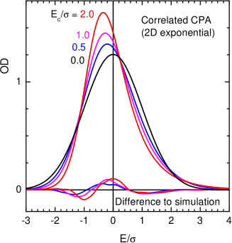
Figure 2: (color online) Optical density for exponentially correlated disorder in two dimensions. CPA calculations in the diagonal version are shown for increasing ratios $E_{c}/\sigma$ (increasing peak height). To judge the quality, differences to the simulation results are shown on the same scale at the bottom.

We begin with a comparison of results in $D=2$ which are relevant for quantum wells with disorder. The correlation type is taken exponential, and we concentrate here and in what follows on the spectral function at ${\bf k}=0$ which gives directly the inhomogeneous broadening of the exciton absorption line, called optical density in the following. Starting with the Gaussian potential distribution in the classical limit ($E_{c}/\sigma=0$), the curves in Fig. 2 are getting more narrow and asymmetric for increasing values of $E_{c}/\sigma$. This represents the motional narrowing on the cm level. The correlated CPA deviates only slightly from the numerically exact results, as visualized by the bottom curves.

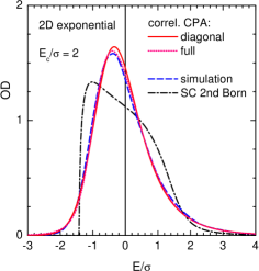
Figure 3: (color online) Optical density for exponentially correlated disorder in two dimensions at $E_{c}/\sigma=2$. Different levels of approximation are compared with the simulation results (see text).

In Fig. 3, we compare the case $E_{c}/\sigma=2$ for different levels of approximations. The self-consistent second Born approximation (dashed-dotted) deviates markedly. Only its high-energy asymptotics is reasonable since it is dominated by perturbation theory. In particular, it fails completely in the low-energy tail where a sharp (square-root) cutoff is produced. This is an inherent feature of any diagrammatic expansion which leads to a geometrical series in terms of the interaction (disorder). The CPA does here pretty well since the final summation over the local potential fluctuations brings in a true random feature. The full version (dotted line, Eq. (21)) gives only a slight improvement compared to the diagonal approximation (full line, Eq. (28)). However, the numerics for the full problem is much more involved since at a given energy, the complete momentum-dependent self-energy has to be brought to convergency. We succeeded only by using acceleration, respectively, slowing down in the recursive determination. On the other hand, the diagonal version needs only a single zero search in the complex plane. Therefore, we show in all the other figures exclusively results from the diagonal version. Then, for the optical density, only $\Sigma_{{\bf k}=0}(z)$ has to be determined self-consistently.

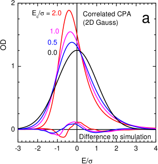
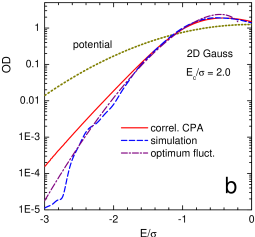
Figure 4: (color online) Optical density for Gauss correlated disorder in two dimensions. In addition to the linear display in (a), the logarithmic display in (b) emphasizes the tail region. The optimum fluctuation result (chained curve) has been adjusted vertically.

It is pleasing to see how the quality of the different approximations (self-consistent second Born, diagonal CPA, and full CPA) goes in parallel to the number of moments which are exactly reproduced. Taking all other parameters unchanged, a correlation of Gauss shape leads to narrower spectral functions compared to the exponential type (Fig. 4(a)). The low-energy tail is shown on a semi-logarithmic plot in Fig. 4(b). The simulation is getting noisy there since states deep in the tail are rare events but compares well with the asymptotically strict result of the optimum fluctuation theory OptFluc , extended here to finite spatial correlation RungeSSP . While the correlated CPA follows initially rather close, deep in the tail the spectral function is somewhat overestimated.

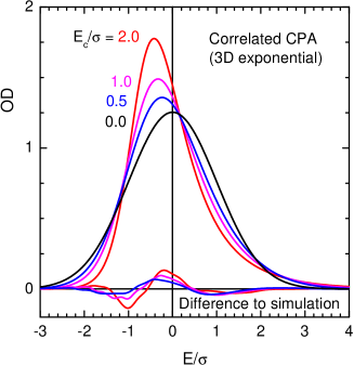
Figure 5: (color online) Optical density for exponentially correlated disorder in three dimensions.

When going from two to three dimensions (Fig. 5), the line width at a given value of $E_{c}/\sigma$ is reduced (cp. Fig. 4(a)). This can be related to the wave-function extension as – loosely speaking – an increased localization length. As well known, it is harder to localize the wave function in $D=3$ compared with $D=2$, assuming the same disorder strength and correlation type. Since we are here interested in states around the lower band edge (these have the dominant contribution to the ${\bf k}=0$ spectral function), the localization edge of the Anderson model in $D=3$ is of no relevance here.

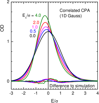
Figure 6: (color online) Optical density for Gauss correlated disorder in one dimension.

To complete the analysis, we show in Fig. 6 results for the one-dimensional problem with Gauss correlated disorder. A final plot (Fig. 7) deals with the uncorrelated case in $D=2$ which is the realm of the standard single-site CPA in the discrete Anderson model. The dispersion to be used here

$$\epsilon_{\bf k}=2T\sum_{j=1}^{2}\left[1-\cos(k_{j}\Delta)\right]$$ (54)

refers to a simple cubic lattice (${\cal N}=\Omega/\Delta^{2}$). The deviations from the (numerically exact) simulation results are definitely smaller than in the correlated cases (Figs. 2 and 4). This is in complete accordance with the moment analysis, since the standard tight-binding CPA for uncorrelated disorder preserves the exact moments even up to $M_{7}({\bf k})$ (we quote the first orders in Appendix C, Eq. (C)). Still, the CPA extension towards correlated potentials is of reasonable quality, and provides therefore a new tool for studying disorder problems in solid state physics.

The present method could be used for the discrete case with spatial correlation as well. The potential generation Eq. (6) has to be discretized as

$$V({\bf R}) = \sum_{{\bf R}^{\prime}}W({\bf R}-{\bf R}^{\prime})\,U({\bf R}^{\prime})\,,$$ (55)

$$\langle U({\bf R})\,U({\bf R}^{\prime})\rangle = \delta_{{\bf R}{\bf R}^{\prime}}$$

where ${\bf R}$ denote the lattice points. All Fourier transforms are restricted to the first Brillouin zone, and in Eqs.(22) and (29) $\epsilon_{\bf k}$ has to be taken as tight-binding dispersion again. However, an application to a binary alloy with spatial correlation (clustering) of the chemical species is not possible: In our method, the (local) potential must be Gauss distributed due to the averaging process Eq. (55), while the relevant correlated potential for the alloy should be still a binary quantity.

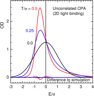
Figure 7: (color online) Optical density (or zero momentum spectral function) in a two-dimensional tight-binding model. The standard CPA result for uncorrelated site disorder is shown and compared with the simulation (here using 2048 Chebychev moments).

Appendix A Analytic properties of the self-energy

The proper Green’s function of the averaged medium $G_{\bf k}(z)$ – considered as a function of the complex-frequency argument $z$ – should obey the following analytic properties (called Herglotz properties, HP Mills ): It is analytic everywhere outside the real axis, obeys the mirror symmetry $G_{{\bf k}}(z^{*})=G^{*}_{{\bf k}}(z)$, and its imaginary part is non negative in the lower half plane. Using physics language, HP guarantee that the Green’s function refers to a causal system, and the spectral function (the jump on the cut along the real axis, see Eq. (30)) is non negative, as appropriate for the probability amplitude for adding a particle with momentum ${\bf k}$ to the system. Due to the simple relation to the self-energy Eq. (16), $\Sigma_{{\bf k}}(z)$ should have HP as well. An alternative formulation is (i) the validity of the spectral representation

$$\Sigma_{{\bf k}}(z)=\int_{-\infty}^{\infty}\frac{d\omega}{\pi}\frac{s_{\bf k}(\omega)}{z-\omega}$$ (56)

with (ii) a non negative spectral density $s_{\bf k}(\omega)\geq 0$. Strictly speaking, a function with HP could have – in addition to the integral in Eq. (56) – a constant and a term linear in $z$. However, in the present case such terms are absent since the self-energy has the virtual crystal as reference. Formally, they are missing in the asymptotic expansion Eq. (45) as well. In the following we will show that the present extension of the CPA to correlated disorder generates a self-energy with Herglotz properties.

The mirror symmetry $\Sigma_{\bf k}^{*}(z)=\Sigma_{\bf k}(z^{*})$ is obvious since – apart from $\Sigma_{{\bf k}}(z)$ and $z$ – only real functions ($\epsilon_{\bf k}$, $g_{\bf k}$, $P(V_{0})$ enter the CPA equations. To be definite we place now $z$ into the lower half plane ($\mbox{\sl Im\,}z<0$) and search for a self-energy with $\mbox{\sl Im\,}\Sigma_{{\bf k}}(z)\geq 0$. Then, it follows at once that the auxiliary function $R_{\bf k}(\hbar z,\{\Sigma\})\equiv R$ defined in Eq. (22) has a positive imaginary part, $R_{2}>0$ (note that $g_{{\bf k}-{\bf k}^{\prime}}$ is non-negative, Eq. (14)). The self consistency condition Eq. (21) is written explicitly as

$$\int dV_{0}\frac{P(V_{0})}{1/R+\Sigma-V_{0}}=R$$ (57)

where $\Sigma\equiv\Sigma_{{\bf k}}(z)$. The integral looks like a standard spectral representation, but the imaginary part of the denominator $D\equiv 1/R+\Sigma-V_{0}$ which is $D_{2}=\Sigma_{2}-R_{2}/|R|^{2}$ may cross zero at some curve in the lower half plane. This would give rise to a non-analytic self-energy there but can indeed never occur: The imaginary part of Eq. (57) reads

$$-D_{2}\int dV_{0}\frac{P(V_{0})}{|D|^{2}}=R_{2}$$ (58)

with a strictly positive value of the integral since $P(V_{0})$ is a positive probability distribution. Therefore, a solution can never have $D_{2}=0$ since $R_{2}>0$ as shown above. This completes the proof that the self-consistent self-energy has HP. The diagonal simplification of Eq. (28) does not change any step of the proof. In this case, the even stronger assertion $D_{2}\leq\hbar z_{2}<0$ holds since the inequality $\mbox{\sl Im\,}(1/R_{\bf k}(\tilde{z})-\hbar\tilde{z})<0$ can be proven quite generally ($\hbar\tilde{z}\equiv\hbar z-\Sigma_{k}(z)$).

In order to see the desired behavior in the numerics as well, we have been searching in the full complex $z$ plane for self-consistent solutions of the self-energy. Indeed, the self-energy was found to vary smoothly as a function of $z$ (crossing non-analytic points/curves would show up as a discontinuity). Still, there could be more than one solution. Assuming at large $|z|$ a vanishing self-energy as initial guess in the root search, we were at least starting with the proper solution, and have continued with the previous solution as start for the next $z$ position. A branching of this solution into two is not possible – this would signal a non-analytic point. However, there could be an accidental degeneracy with a second solution. Although this never occurred in our calculations, we could imagine how to select numerically the proper continuation (demanding the absence of breaks in slope). We were not able to give a general proof for the uniqueness of the solution, as done by Mills and co-workers in Ref.Mills for the substitutional alloy with uncorrelated disorder, and in Ref.Mills84 for a chain with randomly placed delta scatterers. A more practical proof for $\Sigma_{\bf k}(z)$ having HP is to check that the generated function obeys the spectral representation Eq. (56). To do so it is sufficient to run the calculation for $z=\omega-i0$ only, since $s_{\bf k}(\omega)\equiv\mbox{\sl Im\,}\Sigma_{\bf k}(\omega-i0)$. The result in Fig. 8 shows a complete agreement between the direct result and the spectral form

$$\mbox{\sl Re\,}\Sigma_{\bf k}(\omega)=\int_{-\infty}^{\infty}\frac{d\omega^{\prime}}{\pi}s_{\bf k}(\omega^{\prime}){\cal P}\frac{1}{\omega-\omega^{\prime}}$$ (59)

where $\cal P$ stands for the principal value. For comparison, we have added in the figure exact self-energy results which follow from the complex Green’s function generated with our simulation technique using Eq. (16).

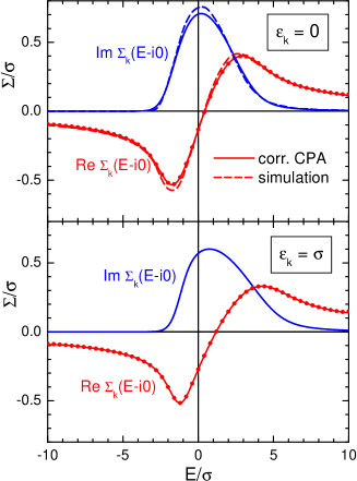
Figure 8: (color online) CPA self-energy for exponential correlation ($E_{c}/\sigma=1$ in two dimensions) at zero momentum (top) and at $\epsilon_{\bf k}=\sigma$ (bottom). The dots give the real part calculated via Eq. (59). The exact self-energy for $\epsilon_{\bf k}=0$ from the simulation is shown dashed.

Appendix B Explicit expressions for different correlation types

The probability distribution of the local potential value $V_{0}$ is of Gauss type, Eq. (17). Therefore, the integral in Eq. (57) can be expressed using the complex error function

$$w(z)=\frac{i}{\pi}\int_{-\infty}^{+\infty}\frac{e^{-t^{2}}dt}{z-t}$$ (60)

resulting in

$$i\sqrt{\frac{2}{\pi}}\sigma R=w\left(\frac{1}{\sqrt{2}\sigma}(1/R+\Sigma_{\bf k}(z)\right)\,.$$ (61)

For the diagonal version, $R\equiv R_{\bf k}(\hbar z-\Sigma_{{\bf k}}(z))$ is understood. The specification of the potential correlation function depends on the system under investigation. If the potential is short-range correlated, we approach the limit of a ”white noise potential” ($g_{\bf k}=1/\Omega$). This is the proper situation for the traditional CPA where the self-energy is assumed to be site diagonal (i.e. independent on momentum ${\bf k}$).

For the exciton case, it is important to note that electron and hole are scanning the potential landscape on a different scale, depending on their masses $m_{e}$ and $m_{h}$. For quantum wells, local fluctuations of the well width $L_{z}$ lead to local shifts of the band edges $E_{a}(L_{z})$, and the smoothing function has the following form TakaRev

$$W({\bf r})=h\zeta\sum_{a=e,h}\eta_{a}^{2}\phi_{1s}^{2}(\eta_{a}{\bf r})\frac{dE_{a}}{dL_{z}}$$ (62)

with mass factors $\eta_{e}=M/m_{h}$ and $\eta_{h}=M/m_{e}$. The parameters $h$ ($\zeta$) characterize typical height (lateral extension) of the well width fluctuations (island size). The exciton wave function can be taken hydrogen like, $\phi_{1s}({\bf r})\propto\exp(-r/a_{B})$, where $a_{B}$ is he appropriate Bohr radius of the quantum well exciton. For equal electron and hole mass ($\eta_{e}=\eta_{h}=2$), Eq. (62) reduces to a single exponential dependence

$$W({\bf r})=\sqrt{\frac{2}{\pi}}\,\frac{\sigma}{\xi}\,e^{-r/\xi}$$ (63)

where $\xi=a_{B}/4$ and

$$\sigma=\sqrt{\frac{2}{\pi}}\frac{h\zeta}{a_{B}}(E^{\prime}_{e}+E^{\prime}_{h})\,.$$ (64)

Performing the two-dimensional integrations we evaluate Eq. (14) with the result

$$g_{\bf k}=\frac{8\pi\xi^{2}}{\Omega}\frac{1}{(1+(k\xi)^{2})^{3}}\,.$$ (65)

The auxiliary function $R_{\bf k}(\hbar z)$ Eq. (29) at ${\bf k}=0$ reads

$$R_{0}(\hbar z)=\int_{0}^{\infty}\!\frac{dx}{\hbar z-E_{c}\,x}\frac{2}{(1+x)^{3}}=\frac{s^{2}+4s+3+2\log(-s)}{E_{c}(1+s)^{3}}$$ (66)

where $s=\hbar z/E_{c}$ is the dimensionless complex energy.

The corresponding results for exponential correlation in quantum wires (one dimension) are

$$g_{\bf k}=\frac{4\xi}{\Omega}\frac{1}{(1+(k\xi)^{2})^{2}}\,,$$ (67)

$$R_{0}(\hbar z) = \frac{4}{\pi}\int_{0}^{\infty}\frac{dx}{(\hbar z-E_{c}\,x^{2})(1+x^{2})^{2}}$$

$$= \frac{s+3-2/\sqrt{-s}}{E_{c}(1+s)^{2}}\,.$$

Finally, we apply Eq. (1) to the bulk mixed crystal and get

$$g_{\bf k}=\frac{64\pi\xi^{3}}{\Omega}\frac{1}{(1+(k\xi)^{2})^{4}}$$ (69)

which is followed by

$$R_{0}(\hbar z) = \frac{32}{\pi}\int_{0}^{\infty}\frac{x^{2}dx}{\hbar z-E_{c}\,x^{2}}\frac{1}{(1+x^{2})^{4}}$$

$$= \frac{s^{3}+5s^{2}+15s-5+16\sqrt{-s}}{E_{c}(1+s)^{4}}\,.$$

For a Gauss-type correlation with characteristic length $\ell$, we assume $W({\bf r})\propto\exp(-r^{2}/2\ell^{2})$ and obtain

$$g_{\bf k}=\frac{1}{\Omega}(2\sqrt{\pi}\ell)^{D}e^{-k^{2}\ell^{2}}\,,$$ (71)

where $D=1,2,3$ is the spatial dimension. The correlation energy is now defined as $E_{c}=\hbar^{2}/(2M\ell^{2})$, and we have to evaluate

$$R_{0}(\hbar z)=\frac{1}{E_{c}\pi^{D/2}}\int_{-\infty}^{+\infty}d^{D}x\,\frac{e^{-x^{2}}}{s-x^{2}}$$ (72)

which gives

$$D=1: R_{0}(\hbar z)=i\frac{\sqrt{\pi}}{E_{c}\sqrt{s}}\,w(-\sqrt{s})\,,$$

$$D=2: R_{0}(\hbar z)=-\frac{e^{-s}}{E_{c}}E_{1}(-s)\,,$$

$$D=3: R_{0}(\hbar z)=\frac{2}{E_{c}}\left(i\sqrt{\pi s}\,w(-\sqrt{s})-1\right)\,.$$

In addition to the complex error function Eq. (60), the exponential integral $E_{1}(z)=\int_{z}^{\infty}dt\,e^{-t}/t$ enters.

Appendix C Result for the exact moments

We list here explicit values for the first exact moments Eq. (36). For Gauss correlation, we take advantage of the closed form

$$K_{n}({\bf k}=0)=E_{c}^{n}\frac{\Gamma(D/2+n)}{\Gamma(D/2)}$$ (74)

in $D$ dimensions, and obtain

$$M_{3} = \sigma^{2}E_{c}\frac{D}{2}\,,$$ (75)

$$M_{4}({\bf k}) = \sigma^{2}E_{c}^{2}\left[\frac{(D+2)D}{4}+2(k\ell)^{2}\right]\,+\,3\,\sigma^{4}\,,$$

$$M_{5}({\bf k}) = \sigma^{2}E_{c}^{3}\frac{D+2}{2}\left[\frac{(D+4)D}{4}+6(k\ell)^{2}\right]\,+\,5D\sigma^{4}E_{c}\,.$$

In the exponential case

$$M_{3}=\sigma^{2}E_{c}$$ (76)

holds independent on spatial dimension. The last finite moment is here

$$M_{4}({\bf k})=\sigma^{2}E_{c}^{2}\left[5+\frac{4}{3}\left(k\xi\right)^{2}\right]\,+\,3\,\sigma^{4}$$ (77)

for $D=3$. This unexpected termination of the moment expansion can be understood quite easily: The spectral function Eq. (30) decays at large positive energies as

$$A_{{\bf k}=0}(\omega)\Rightarrow\sum_{\bf k}\frac{\sigma^{2}g_{\bf k}}{\epsilon_{\bf k}^{2}}\pi\delta(\hbar\omega-\epsilon_{\bf k})$$ (78)

which follows from plain perturbation theory using Eq. (27) in leading order. For the Gauss correlation Eq. (71), multiplication with any power of $\hbar\omega=\epsilon_{\bf k}$ leads to a convergent frequency (better momentum) integral. For the exponential case, however, we have $g_{{\bf k}}\propto k^{-(2D+2)}$, and the integrand of the $n$th moment behaves as $k^{(2n-D-7)}$. Therefore, the moments are finite up to $n=3$ ($D=1,2$) or $n=4$ ($D=3$).

For the sake of completeness, we quote the moments in the uncorrelated (tight-binding) case as well. $M_{0}=1$, $M_{1}=0$, and $M_{2}=\sigma^{2}$ hold as before. We write the (simple cubic) dispersion as

$$\epsilon_{\bf k}=2TD\left(1-C({\bf k})\right)\,,\;\;C({\bf k})=\frac{1}{D}\sum_{j=1}^{D}\cos(k_{j}\Delta)$$ (79)

and obtain instead of Eqs. (41)-(43)

$$M_{3}({\bf k}) = 2TD\sigma^{2}C({\bf k})\,,$$

$$M_{4}({\bf k}) = (2TD)^{2}\sigma^{2}\left(C^{2}({\bf k})+\frac{1}{2D}\right)+3\sigma^{4}\,,$$ (80)

$$M_{5}({\bf k}) = C({\bf k})\left\{(2TD)^{3}\sigma^{2}\left(C^{2}({\bf k})+\frac{3}{2D}\right)+16TD\sigma^{4}\right\}\,.$$

References

- (1) P. Soven, Phys. Rev. 156, 809 (1967).
- (2) B. Velicky, S. Kirkpatrick, and H. Ehrenreich, Phys. Rev. 175, 747 (1968).
- (3) B. Velicky, Phys. Rev. 184, 614 (1969).
- (4) Yu-Tang Shen and Ch. W. Myles, Phys. Rev. B 30, 3283 (1984).
- (5) T. P. Eggarter and A. Troper, Phys. Status Solidi B 140, 127 (1987).
- (6) R. Mills and P. Ratanavararaksa, Phys. Rev. B 18, 5291 (1978); R. Mills, L. J. Gray, and Th. Kaplan, Phys. Rev. B 27, 3252 (1983).
- (7) A. Mookerjee and R. Prasad, Phys. Rev. B 48, 17724 (1993).
- (8) M. Jarrell and H. R. Krishnamurthy, Phys. Rev. B 63, 125102 (2001).
- (9) Th. Maier, M. Jarrell, Th. Pruscheke, and M. H. Hettler, Rev. Mod. Phys. 77, 1027 (2005).
- (10) D. A. Rowlands, J. Phys.: Condens. Matter 18, 3179 (2006).
- (11) M.S. Laad and L. Craco, J. Phys.: Condens. Matter 17, 4765 (2005).
- (12) A. Weiße, G. Wellein, A. Alvermann, and H. Fehske, Rev. Modern Physics 78, 275 (2006).
- (13) S. D. Baranovskii and A. L. Efros, Sov. Phys. Semicond., 12, 1328 (1978).
- (14) R. Zimmermann, J. Crystal Growth 101, 346 (1990).
- (15) S. M. Lee and K. K. Bajaj, Appl. Phys. Lett. 60, 853 (1992).
- (16) S. K. Lyo, Phys. Rev. B 48, 2152 (1993).
- (17) M. A. Kanehisa and R. J. Elliott, Phys. Rev. B 35, 2228 (1987).
- (18) D. L. Huber and W. Y. Ching, Phys. Rev. B 39, 8652 (1989).
- (19) P. Reineker, J. Köhler, and A. M. Jayannavar, J. Lumin. 45, 102 (1990).
- (20) F. Dominguez-Adame, Phys. Rev. B 51, 12801 (1995).
- (21) L. D. Bakalis, I. Rubtsov, and J. Knoester, J. Chem. Physics 117, 5393 (2002).
- (22) S. Glutsch, D. S. Chemla, and F. Bechstedt Phys. Rev. B 54, 11592 (1996).
- (23) R. Zimmermann, E. Runge, and V. Savona: Theory of resonant secondary emission: Rayleigh scattering versus luminescence In: Quantum Coherence, Correlation and Decoherence in Semiconductor Nanostructures (T. Takagahara ed.), p. 89-165, Elsevier Science (USA), 2003.
- (24) V. Savona and R. Zimmermann, Phys. Rev. B 60, 4928 (1999).
- (25) Ch. Lienau, F. Intonti, T. Guenther, Th. Elsaesser, V. Savona, R. Zimmermann, and E. Runge, Phys. Rev. B 69, 085302 (2004).
- (26) E. Runge, Solid State Physics Vol. 57, (H. Ehrenreich and F. Saepen ed.), p. 149-305, Academic Press, San Diego, 2002.
- (27) M. Grochol, F. Grosse, and R. Zimmermann, Phys. Rev. B 71, 125339 (2005).
- (28) R. H. Kraichnan, Phys. Rev. 109, 1407 (1958).
- (29) T. Stroucken, C. Anthony, A. Knorr, P. Thomas, and S. W. Koch, Phys. Status Solidi B 188, 539 (1995).
- (30) St. Glutsch and F. Bechstedt, Phys. Rev. B 50, 7733 (1994).
- (31) M. Vogt, R. Zimmermann, and R. J. Needs, Phys. Rev. B 69, 045113 (2004).
- (32) I. M. Lifshits, S. A. Gredeskul, and L. A. Pastur, Introduction to the Theory of Disordered systems, Wiley, New York, 1988.
- (33) A. K. Sen, R. Mills, Th. Kaplan, and L. J. Gray, Phys. Rev. B 30, 5686 (1984).