Compressed Remote Sensing of Sparse Objects

Abstract.

The linear inverse source and scattering problems are studied from the perspective of compressed sensing, in particular the idea that sufficient incoherence and sparsity guarantee uniqueness of the solution. By introducing the sensor as well as target ensembles, the maximum number of recoverable targets (MNRT) is proved to be at least proportional to the number of measurement data modulo a log-square factor with overwhelming probability.

Important contributions include the discoveries of the threshold aperture, consistent with the classical Rayleigh criterion, and the decoherence effect induced by random antenna locations.

The prediction of theorems are confirmed by numerical simulations.

1. Introduction

We consider the imaging problem in the form of inverse source or scattering problem which has wide-range applications such as radar, sonar and computed tomography. The imaging problem is typically plagued by nonuniqueness and instability and hence mathematically challenging. Traditional methods such as matched field processing  [25] are limited in the number of targets that can be reliably recovered at high resolution. They often fail to detect a substantial number of targets, while at the same time they tend to produce artifacts obscuring the real target images. These limitations are due to the presence of noise and the fact that the imaging problem is in practice underdetermined. The standard regularization methods can handle to some extent the problem with noise but are inadequate to remedy the issue of nonuniqueness of the solution.

In this paper we utilize the fact that in many imaging applications the targets are sparse in the sense that they typically occupy a small fraction of the overall region of interest (the target domain). This sparsity assumption suggests to approach the imaging problem by using the framework of compressed sensing.

At the core of compressed sensing lies the following problem (here we focus, as is common in the compressed sensing community, on the discrete setting). Assume $X\in\mathbb{C}^{m}$ is a signal that is sparse, i.e., the number of its non-zero components (measured by the $\ell_{0}$-quasinorm $\|X\|_{0}$ which is simply the number of non-zero entries of $X$) satisfies $s:=\|X\|_{0}\ll m$. Let $Y\in\mathbb{C}^{n}$ be the measurement data vector. We explore in this paper the linear inverse problem which can be formulated as $Y=\mathbf{A}X$ where $\mathbf{A}$ is an $n\times m$ matrix with $n\ll m$. The goal is to recover $X$, given the data vector $Y$ and the sensing matrix $\mathbf{A}$ of full rank. As $n\ll m$, $\mathbf{A}X=Y$ is severely underdetermined and unique reconstruction of $X$ is in general impossible.

However, due to the sparsity of $X$ one can compute $X$ by solving the optimization problem

(L0) $$\min\|X\|_{0}\qquad\text{s.t.}\,\,\mathbf{A}X=Y.$$

Since (L0) is NP-hard and thus computationally infeasible, we consider instead its convex relaxation, also known as Basis Pursuit (BP),

(L1) $$\min\|X\|_{1}\qquad\text{s.t.}\,\,\mathbf{A}X=Y$$

which can be solved by linear and quadratic programming techniques. The amazing discovery due to David Donoho was that under certain conditions on the matrix $\mathbf{A}$ and the sparsity of $X$, both (L1) and (L0) have the same unique solution [14]. One such condition is the Restricted Isometry Property (RIP) due to Candes and Tao [7], which requires essentially that any $n\times s$ submatrix of $\mathbf{A}$ is an approximate isometry. This property is satisfied by a number of matrices such as Gaussian random matrices or random partial Fourier matrices [7, 5, 24]. In that case, as long as $s\leq{\mathcal{O}}(n/\log(m))$, with high probability the solution of (L1) will indeed coincide with the solution of (L0). Another conditon for which equivalence between (L0) and (L1) can be proven is based on the incoherence of the columns of $\mathbf{A}$, which refers to the property that the inner product of any two columns of $\mathbf{A}$ is small [12, 17, 26]. Moreover, the performance of BP is stable w.r.t. the presence of noise and error [6, 13, 27]. Finally the computational complexity of BP can be significantly reduced by using the various greedy algorithms in place of the linear programming technique [9, 21, 22, 26, 27]. The most basic greedy algorithm relevant here is Orthogonal Matching Pursuit (OMP) which has been thoroughly analyzed in [26].

For the imaging problem, the sensing matrix $\mathbf{A}$ represents a physical process (typically wave propagation) and thus its entries cannot be arbitrarily chosen at our convenience. Therefore we cannot simply assume that $\mathbf{A}$ satisfies any of the conditions that make compressed sensing work. The few physical parameters that we have control over are the wavelength $\lambda$ of the probe wave, the locations and number $n$ of sensors and the aperture $A$ of the probe array. This is one of the reasons that make the practical realization of compressed sensing a challenging task.

The paper is organized as follows. In Section 2 we describe the physical setup, formulate the imaging problem in the framework of compressed sensing and make qualitative statements of our main results. In Section 3 we prove the main result for the inverse source problem, in particular the coherence estimate (Section 3.1) and the spectral norm bound (Section 3.2). In Section 4, we prove the main result for the inverse Born scattering problem for the response matrix imaging (Section 4.1) and the synthetic aperture imaging (Section 4.2). In Section 5 and Appendix B, we discuss the numerical method and present simulation results that confirm qualitatively the predictions of our theorems. In Appendix A we discuss the RIP approach to our problems.

2. Problem formulations and main results

In this paper, we study the inverse source and scattering problems both in the linear regime to suit the current framework of compressed sensing. For simplicity and definiteness we consider the three dimensional space and assume that all targets are in the transverse plane $\{z=z_{0}\}$ and all sensors are in another transverse plane $\{z=0\}$. The exact Green function for the Helmholtz equation which governs the monochromatic wave propagation is

(1) $$G(\mathbf{r},{\mathbf{a}})={e^{i\omega|\mathbf{r}-{\mathbf{a}}|}\over 4\pi|\mathbf{r}-{\mathbf{a}}|},\quad\mathbf{r}=(x,y,z_{0}),\quad{\mathbf{a}}=(\xi,\eta,0).$$

We assume that the phase speed $c=1$ so that the frequency $\omega$ equals the wavenumber.

We consider the Fresnel diffraction regime where the distance $z_{0}$ between the targets and the sensors is much larger than the wavelength of the probe wave and the linear dimensions of the domains [3]

(2) $$z_{0}\gg A+L,\quad z_{0}\gg\lambda$$

where $L$ is the linear dimension of the target domain. This is the remote sensing regime.

Under (2) the Green function (1) can be approximated by the universal parabolic form [3]

(3) $$G(\mathbf{r},{\mathbf{a}})={e^{i\omega z_{0}}\over 4\pi z_{0}}e^{i\omega|x-\xi|^{2}/(2z_{0})}e^{i\omega|y-\eta|^{2}/(2z_{0})},$$

which is called the paraxial Green function. This follows from the truncated Taylor expansion of the function $|\mathbf{r}-{\mathbf{a}}|$

$$|\mathbf{r}-{\mathbf{a}}|\approx z_{0}+{|x-\xi|^{2}\over 2z_{0}}+{|y-\eta|^{2}\over 2z_{0}}$$

under (2).

In the case of the inverse source problem, the corresponding sensing matrix $\mathbf{A}$ is essentially made of the paraxial Green function for various points in the sensor array and the target domain. In this set-up, the entries (3) of the paraxial sensing matrix have the same magnitude so without loss of generality the column vectors of $\mathbf{A}$ are assumed to have unit $\ell^{2}$-norm.

A key idea in our construction of a suitable sensing matrix is to randomize the locations ${\mathbf{a}}_{j}=(0,\xi_{j},\eta_{j}),j=1,...,n$ of the $n$ sensors within a fixed aperture (a square of size $A$ for example). Indeed, we assume $\xi_{j},\eta_{j}$ are independent uniformly distributed in $[0,A]$. We assume that the antenna elements are independently uniformly distributed in a square array $[0,A]\times[0,A]$ in the plane $\{z=0\}$. Define the sensor ensemble to be the sample space of $n$ i.i.d. uniformly distributed points in $[0,A]^{2}$.

We consider the idealized situation where the locations of the targets are a subset of a square lattice. More precisely, let ${\mathcal{M}}$ be a regular square sub-lattice ${\mathcal{M}}=\left\{\mathbf{r}_{i}:i=1,...,m\right\}$ of mesh size $\ell$ in the transverse plane $\{z=z_{0}\}$. Hence the total number of grid points $m$ is a perfect square. We defer the discussion on extended targets to the concluding section.

Let ${\mathcal{S}}=\left\{\mathbf{r}_{j_{l}}:l=1,...,s\right\}$ be the set of target locations and $\sigma_{j_{l}},l=1,...,s$ be the (source or scattering) amplitudes of the targets. Set $\sigma_{i}=0,i\not\in\{j_{1},...,j_{s}\}$. Define the target vector $X$ to be $X=(\sigma_{j})\in\mathbb{C}^{m}$. We consider the target ensemble consisting of target vectors with at most $s$ non-zero entries whose phases are independently, uniformly distributed in $[0,2\pi]$ and whose support indices are independently and randomly selected from the index set $\{1,2,...,m\}$. The number $s=\|X\|_{0}$ is called the sparsity of the target vector.

For source inversion the targets emit the paraxial waves described by (3) which are then recorded by the sensors. The measurement vector $Y$ can be written as

(4) $$Y=\mathbf{A}X$$

where the matrix $\mathbf{A}=[A_{ij}]\in\mathbb{C}^{n\times m}$ have the entries

(5) $$A_{ij}=G({\mathbf{a}}_{i},\mathbf{r}_{j}),\quad\forall i=1,...,n,\quad j=1,...,m.$$

The first main result proved in this paper can be stated roughly as follows (see Theorem 2 and Remark 3 for the precise statement).

Result A. Suppose

(6) $${\ell A\over\lambda z_{0}}\equiv{1\over\rho}\in\mathbb{N}.$$

For the product ensemble of targets and sensors, sources of sparsity up to ${\mathcal{O}}(n/(\ln{m})^{2})$ can be exactly recovered by BP with overwhelming probability.

When only the sensor ensemble is considered, all sources of sparsity up to ${\mathcal{O}}(\sqrt{n})$ can be exactly recovered by BP and OMP with overwhelming probability.

The relation (6) indicates the existence of the threshold, optimal aperture given by $\lambda z_{0}/\ell$ corresponding to $\rho=1$ (see Remark 2 for more discussion on this point). Since the meshsize $\ell$ has the meaning of resolution, $\rho=1$ is consistent with the classical Rayleigh criterion [3]

(7) $$\ell\geq{\lambda z_{0}\over A}.$$

Our numerical simulations (Figure 1) indeed indicate that (7) is sufficient to realize the performance stated in Result A.

Next we consider two imaging settings where the targets are scatterers instead of sources. For point scatterers of amplitudes $\sigma_{j_{l}}$ located at $\mathbf{r}_{j_{l}},l=1,2,3,...s$, the resulting Green function $\tilde{G}$, including the multiple scattering effect, obeys the Lippmann-Schwinger equation

$$\tilde{G}(\mathbf{r},{\mathbf{a}}_{i})=G(\mathbf{r},{\mathbf{a}}_{i})+\sum_{l=1}^{s}\sigma_{j_{l}}G(\mathbf{r},\mathbf{r}_{j_{l}})\tilde{G}(\mathbf{r}_{j_{l}},{\mathbf{a}}_{i}),\quad i=1,...,n.$$

The exciting field $\tilde{G}(\mathbf{r}_{j_{l}},{\mathbf{a}}_{i})$ is part of the unknown and can be solved for from the so called Foldy-Lax equation (see e.g. [15] for details).

Hence, the inverse scattering problem is intrinsically nonlinear. However, often linear scattering model is a good approximation and widely used in, e.g. radar imaging in the regimes of physical optics and geometric optics [2, 8] (see [29] for a precise formulation of the condition).

One such model is the Born approximation (also known as Rayleigh-Gans scattering in optics) in which the unknown exciting field is replaced by the incident field resulting in

(8) $$\tilde{G}(\mathbf{r},{\mathbf{a}}_{i})-G(\mathbf{r},{\mathbf{a}}_{i})=\sum_{l=1}^{s}\sigma_{j_{l}}G(\mathbf{r},\mathbf{r}_{j_{l}})G(\mathbf{r}_{j_{l}},{\mathbf{a}}_{i}),\quad i=1,...,n.$$

The left hand side of (8) is precisely the scattered field when the incident field is emitted from a point source at ${\mathbf{a}}_{i}$. The Born approximation linearizes the relation between the scatterers and the scattered field. The goal of inverse scattering is to reconstruct the targets given the measurements of the scattered field.

For the response matrix (RM) imaging [15, 16], we use the real array aperture as in the inverse source problem discussed above except the array is also the source of $n$ probe waves. One by one, each antenna of the array emits an impulse and the entire array receives the echo. Each transmitter-receiver pair gives rise to a datum and there are altogether $n^{2}$ data forming a datum matrix called the response matrix. These data represent the responses of the targets to the interrogating waves.

From (8) we see that the corresponding sensing matrix $\mathbf{A}^{\rm RM}$ has the entries

$$A^{\rm RM}_{lj}=G({\mathbf{a}}_{i},\mathbf{r}_{j})G(\mathbf{r}_{j},{\mathbf{a}}_{k}),\quad l=1,..,n^{2},\quad j=1,...,m$$

where $l$ is related to $i,k$ as

$$l=i(n-1)+k.$$

In the second setting, called the synthetic aperture (SA) imaging, the real, physical array consists of only one antenna. The imaging aperture is synthesized by the antenna taking different transmit-receive positions ${\mathbf{a}}_{i},i=1,...,n$ [16].

The SA imaging considered here is motivated by synthetic aperture radar (SAR) imaging. SAR is a technique where a substantial aperture can be synthesized by moving a transmit-receive antenna along a trajectory and repeatedly interrogating a search area by firing repeated pulses from the antenna and measuring the responses. This can greatly leverage a limited probe resource and has many applications in remote sensing. The image formation is typically obtained via the matched filter technique and analyzed in the Born approximation [8].

Here we consider a simplified set-up, neglecting the Doppler effect associated with the relative motion between the antenna and targets. In this case, the sensing matrix $\mathbf{A}^{\rm SA}$ has the entries

(9) $$A^{\rm SA}_{ij}=G^{2}({\mathbf{a}}_{i},\mathbf{r}_{j}),\quad i=1,...,n,\quad j=1,...,m.$$

In other words, $A^{\rm SA}_{ij}=A^{\rm RM}_{lj}$ with $l=i(n-1)+i.$ A crucial observation about SA imaging is that

(10) $$G^{2}({\mathbf{a}}_{i},\mathbf{r}_{j};\omega)\sim G({\mathbf{a}}_{i},\mathbf{r}_{j};2\omega)$$

modulo a $z_{0}$-dependent factor which does not matter.

The following is a rough statement for inverse Born scattering (Theorems 7, 8 and Remarks 4, 5) proved in Section 4.

Result B. (i) For RM imaging, assume the aperture condition (6).

For the product ensemble of sensor and target, scatterers of sparsity up to ${\mathcal{O}}(n^{2}/(\ln{m})^{2})$ can be reconstructed exactly by BP with overwhelming probability.

When only the sensor ensemble is considered, all scatterers of sparsity up to ${\mathcal{O}}(n)$ can be exactly recovered by BP and OMP with overwhelming probability.

(ii) For SA imaging, assume the aperture condition

(11) $$2/\rho\in\mathbb{N}$$

which is weaker than (6).

For the product ensemble of sensor and target, scatterers of sparsity up to ${\mathcal{O}}(n/(\ln{m})^{2})$ can be reconstructed exactly by BP with overwhelming probability.

When only the sensor ensemble is considered, all scatterers of sparsity up to ${\mathcal{O}}(\sqrt{n})$ can be exactly recovered by BP and OMP with overwhelming probability.

As a result of the SA aperture condition (11), the corresponding optimal aperture is half of that for the inverse source and RM imaging. In other words, SA can produce the qualitatively optimal performance with half of the aperture. This two-fold enhancement of resolving power in SA imaging has been previously established for the matched-field imaging technique [16].

Our numerical simulations (Section 5) confirm qualitatively the predictions of Result A and B, in particular the threshold aperture and the asymptotic number of recoverable targets.

Currently there are two avenues to compressed sensing [4]: the incoherence approach and the RIP (restricted isometry property) approach. When the RIP approach works, the results are typically superior in that all targets under a slightly weaker sparsity constraint can be uniquely determined by BP without introducing the target ensemble. We demonstrate the strength of the RIP approach for our problems in Appendix A (see Theorem 11 and Theorem 12 for stronger results than Result A and Result B (ii), respectively). However, Result B(i) seems unattainable by the RIP approach at present, particularly the quadratic-in-$n$ behavior of the sparsity constraint. On the other hand, the incoherence approach gives a unified treatment to all three results and therefore is adopted in the main text of the paper.

3. Source inversion

Let $G(\mathbf{r},{\mathbf{a}})$ be the Green function of the time-invariant medium and let ${\mathbf{G}}$ be the Green vector

(12) $${\mathbf{G}}(\mathbf{r})=[G(\mathbf{r},{\mathbf{a}}_{1}),G(\mathbf{r},{\mathbf{a}}_{2}),...,G(\mathbf{r},{\mathbf{a}}_{n})]^{t}$$

where $t$ denotes transpose. For the matrix (5) define the coherence of the matrix $\mathbf{A}$ by

$$\mu(\mathbf{A})=\max_{i\neq j}{\left|{\mathbf{G}}^{*}(\mathbf{p}_{i}){\mathbf{G}}(\mathbf{p}_{j})\right|\over\|{\mathbf{G}}(\mathbf{p}_{i})\|\|{\mathbf{G}}(\mathbf{p}_{j})\|}.$$

The following theorem is a reformulation of results due to Tropp [28] and the foundation of the imaging techniques developed in this paper.

Theorem 1.

Let $X$ be drawn from the target ensemble. Assume that

(13) $$\mu^{2}s\leq\left(8\ln{{m\over\epsilon}}\right)^{-1},\quad\epsilon\in(0,1)$$

and that for $p\geq 1$

(14) $$3\left({p\ln{s}\over 2\ln{{m\over\epsilon}}}\right)^{1/2}+{s\over m}\|\mathbf{A}\|_{2}^{2}\leq{1\over 4e^{1/4}}.$$

Then $X$ is the unique solution of BP with probability $1-2\epsilon-s^{-p}$. Here $\|\mathbf{A}\|_{2}$ denotes the spectral norm of $\mathbf{A}$.

We explain the connection of the theorem with [28] in Appendix B.

Theorem 2.

Let the target vector be randomly drawn from the target ensemble and the antenna array be randomly drawn from the sensor ensemble and suppose

(15) $${\ell A\over\lambda z_{0}}\equiv{1\over\rho}\in\mathbb{N}.$$

If

(16) $$m\leq{\delta\over 2}e^{K^{2}/2},\quad\delta,K>0.$$

then the targets of sparsity up to

(17) $$s<{n\over 64\ln{2m\over\delta}\ln{m\over\epsilon}}$$

can be recovered exactly by BP with probability greater than or equal to

(18) $$\left[1-2\delta-{\rho n(n-1)^{3/2}\over m^{1/2}}\right]\times\left[1-2\epsilon-s^{-p}\right],\quad p={\ln{m}-\ln{\epsilon}\over 288\sqrt{e}\ln s}.$$

Proof.

The proof of the theorem hinges on the following two estimates.

Theorem 3.

Assume (15) and

(19) $$m\leq{\delta\over 2}e^{K^{2}/2}$$

for some positive $\delta$ and $K$. Then the coherence of $\mathbf{A}$ satisfies

(20) $$\mu(\mathbf{A})\leq\sqrt{2}K/\sqrt{n}$$

with probability greater than $(1-\delta)^{2}$.

Remark 1.

The general lower bound for coherence [10, 30]

$$\sqrt{m-n\over n(m-1)}\leq\mu\leq 1$$

implies that the coherence bound (20) is optimal modulo a constant factor.

Remark 2.

Since the coherence of the sensing matrix should decrease as the aperture increases and since the analysis in Section 3.1 shows that the coherence is of the same order of magnitude as $n^{-1/2}$ whenever (15) holds, simple interpolation leads to the conclusion that the coherence should be roughly constant for

(21) $$A\geq{\lambda z_{0}\over\ell}$$

corresponding to $\rho\leq 1$. The right hand side of (21), corresponding to $\rho=1$, defines the optimal aperture.

Theorem 4.

The matrix $\mathbf{A}$ has full rank and its spectral norm satisfies the bound

(22) $$\|\mathbf{A}\|_{2}^{2}\leq 2m/n$$

with probability greater than

(23) $$1-{\rho n(n-1)^{3/2}\over m^{1/2}},\quad\rho={\lambda z_{0}\over\ell A}.$$

Remark 3.

By the theorems of Donoho, Elad [12] and Tropp [26], the targets of sparsity

$$s<{1\over 2}(1+{1\over\mu(\mathbf{A})})$$

can be recovered exactly by BP as well as by Orthogonal Matching Pursuit (OMP).

Theorems 3 and 4 imply that with probability greater than

$$1-2\delta-{\rho n(n-1)^{3/2}\over m^{1/2}}$$

of the sensor ensemble, all targets of sparsity

$$s<{1\over 2}(1+{\sqrt{n}\over\sqrt{2}K})$$

can be recovered exactly by BP as well as OMP.

Condition (17) implies the existence of $K$ such that

(24) $$2\ln{2m\over\delta}<K^{2}<{n\over 32s\ln{m\over\epsilon}}.$$

As a consequence (19) and (13) are satisfied with probability greater than $1-2\delta$ by Theorem 3.

Now the norm bound (22) implies (14) if

(25) $$3\left({p\ln{s}\over 2\ln{{m\over\epsilon}}}\right)^{1/2}+{2s\over n}\leq{1\over 4e^{1/4}},\quad p>1,$$

which in turn follows from (17) and the condition

$$\ln{2m\over\delta}\ln{m\over\epsilon}\geq{1\over 96}\left({1\over 2e^{1/4}}-\left(p\ln s\over 2\ln{m\over\epsilon}\right)^{1/2}\right)^{-1}.$$

Hence for $m\gg s$ (and hence $n\gg s$) we can choose $p$ in (14) to be

$$p={\ln{m}-\ln{\epsilon}\over 72\sqrt{e}\ln s}.$$

Since Theorems 3 and 4 hold with probability greater than

$$1-2\delta-{\rho n(n-1)^{3/2}\over m^{1/2}}.$$

and since the target ensemble is independent of the sensor ensemble we have the bound (18) for the probability of exact recovery.

∎

3.1. Proof of Theorem 3: coherence estimate

Proof.

Summing over ${\mathbf{a}}_{l},l=1,...,n$ we obtain

(26) $$\sum_{l=1}^{n}A^{*}_{li}A_{lj} = e^{i\omega(x_{j}^{2}+y_{j}^{2}-x_{i}^{2}-y_{i}^{2})/(2z_{0})}{1\over n}\sum_{l=1}^{n}e^{i\xi_{l}\omega(x_{i}-x_{j})/z_{0}}e^{i\eta_{l}\omega(y_{i}-y_{j})/z_{0}}.$$

Define the random variables $X_{l},Y_{l},l=1,...,n$, as

(27) $$X_{l} = \cos{\left[(\xi_{l}(x_{i}-x_{j})+\eta_{l}(y_{i}-y_{j}))\omega/z_{0}\right]}$$

(28) $$Y_{l} = \sin{\left[(\xi_{l}(x_{i}-x_{j})+\eta_{l}(y_{i}-y_{j}))\omega/z_{0}\right]}$$

and their respective sums

$$S_{n}=\sum_{l=1}^{n}X_{l},\quad T_{n}=\sum_{l=1}^{n}Y_{l}.$$

Then the absolute value of the right hand side of (26) is bounded by

(29) $${1\over n}\left|S_{n}+iT_{n}\right|\leq{1\over n}\left(\left|S_{n}-\mathbb{E}S_{n}\right|+\left|T_{n}-\mathbb{E}T_{n}\right|+\left|\mathbb{E}(S_{n}+iT_{n})\right|\right).$$

To estimate the right hand side of (29), we recall the Hoeffding inequality [20].

Proposition 1.

Let $X_{1},...,X_{n}$ be independent random variables. Assume that $X_{l}\in[a_{l},b_{l}],l=1,...,n$ almost surely. Then we have

(30) $$\mathbb{P}\left[\left|S_{n}-\mathbb{E}S_{n}\right|\geq nt\right]\leq 2\exp{\left[-{2n^{2}t^{2}\over\sum_{l=1}^{n}(b_{l}-a_{l})^{2}}\right]}$$

for all positive values of $t$.

We apply the Hoeffding inequality to both $S_{n}$ and $T_{n}$. To this end, we have $a_{l}=-1,b_{l}=1,\forall l$ and set

$$t=K/\sqrt{n},\quad K>0.$$

Then we obtain

(31) $$\mathbb{P}\left[n^{-1}\left|S_{n}-\mathbb{E}S_{n}\right|\geq K/\sqrt{n}\right] \leq 2e^{-{K^{2}/2}}$$

(32) $$\mathbb{P}\left[n^{-1}\left|T_{n}-\mathbb{E}T_{n}\right|\geq K/\sqrt{n}\right] \leq 2e^{-{K^{2}/2}}.$$

Note that the quantities $S_{n},T_{n}$ depend on $x_{i}-x_{j},y_{i}-y_{j}$, i.e.

$$S_{n}=S_{n}(x_{i}-x_{j},y_{i}-y_{j}),\quad T_{n}=T_{n}(x_{i}-x_{j},y_{i}-y_{j}).$$

We use (31)-(32) and the union bound to obtain

(33) $${\mathbb{P}\left[\max_{i\neq j}n^{-1}\left|S_{n}(x_{i}-x_{j},y_{i}-y_{j})-\mathbb{E}S_{n}(x_{i}-x_{j},y_{i}-y_{j})\right|\geq K/\sqrt{n}\right]}$$

$$\hskip 28.45274pt\leq 2(m-1)e^{-K^{2}/2}$$

(34) $${\mathbb{P}\left[\max_{i\neq j}n^{-1}\left|T_{n}(x_{i}-x_{j},y_{i}-y_{j})-\mathbb{E}T_{n}(x_{i}-x_{j},y_{i}-y_{j})\right|\geq K/\sqrt{n}\right]}$$

$$\hskip 28.45274pt\leq 2(m-1)e^{-K^{2}/2}$$

Hence, if (19) holds for any small number $\delta>0$, then the right hand side of (33)-(34) is less than $\delta$.

The third term on the right hand side of (29) can be calculated as follows. By the mutual independence of $\xi_{l}$ and $\eta_{l}$ we have

$${1\over n}\left|\mathbb{E}(S_{n}+iT_{n})\right| = {1\over n}\left|\sum_{l=1}^{n}\mathbb{E}(X_{l}+iY_{l})\right|$$

$$= {1\over n}\left|\sum_{l=1}^{n}\mathbb{E}\left(e^{i\xi_{l}\omega(x_{i}-x_{j})/z_{0}}\right)\mathbb{E}\left(e^{i\eta_{l}\omega(y_{i}-y_{j})/z_{0}}\right)\right|$$

$$= \left|\mathbb{E}\left(e^{i\xi_{l}\omega(x_{i}-x_{j})/z_{0}}\right)\mathbb{E}\left(e^{i\eta_{l}\omega(y_{i}-y_{j})/z_{0}}\right)\right|$$

since $\xi_{l},\eta_{l},l=1,...,n$ are independently identically distributed.

Simple calculation with the uniform distribution on $[0,A]\times[0,A]$ yields

(35) $$\left|\mathbb{E}\left(e^{i\xi_{l}\omega(x_{i}-x_{j})/z_{0}}\right)\mathbb{E}\left(e^{i\eta_{l}\omega(y_{i}-y_{j})/z_{0}}\right)\right| = \left|{e^{i\phi_{ij}}-1\over\phi_{ij}}\right|\left|{e^{i\psi_{ij}}-1\over\psi_{ij}}\right|$$

$$= 4\left|{\sin{{\phi_{ij}}\over 2}\over\phi_{ij}}\right|\left|{\sin{\psi_{ij}\over 2}\over\psi_{ij}}\right|$$

with

$$\phi_{ij}=A\omega(x_{i}-x_{j})/z_{0},\quad\psi_{ij}=A\omega(y_{i}-y_{j})/z_{0}.$$

The optimal condition is to choose $A$ such that

(36) $$\phi_{ij}=\psi_{ij}\in 2\pi\mathbb{Z},$$

under which (35) vanishes. Condition (36) can be fulfilled for an equally spaced grid as is assumed here. Let

$$\ell=\min_{i\neq j}|x_{i}-x_{j}|=\min_{i\neq j}|y_{i}-y_{j}|.$$

The smallest $\ell$ satisfying condition (36) is given by

(37) $$\ell={z_{0}\lambda\over A},\quad\lambda=2\pi/\omega$$

which can be interpreted as the resolution of the imaging system and is equivalent to the classical Rayleigh criterion.

In this case, $\mathbb{E}(S_{n}+iT_{n})=0$ and hence

$$\mu(\mathbf{A})\leq\sqrt{2}K/\sqrt{n}$$

with probability $(1-\delta)^{2}$ under the condition (19).

∎

3.2. Proof of Theorem 4: spectral norm bound

Proof.

For the proof, it suffices to show that the matrix $\mathbf{A}$ satisfies

(38) $$\|{n\over m}\mathbf{A}\mathbf{A}^{*}-\mathbf{I}_{n}\|_{2}<1$$

where $\mathbf{I}_{n}$ is the $n\times n$ identity matrix with the corresponding probability bound. By the Gershgorin circle theorem, (38) would in turn follow from

(39) $$\mu\left(\sqrt{n\over m}\mathbf{A}^{*}\right)<{1\over n-1}$$

since the diagonal elements of ${n\over m}\mathbf{A}\mathbf{A}^{*}$ are unity.

Since $(\xi_{i},\eta_{i}),i=1,...,n$ are uniformly distributed in $[0,A]\times[0,A]$, $\xi_{i}\neq\xi_{j},\eta_{i}\neq\eta_{j}$ with probability one.

Summing over $\mathbf{r}_{l},l=1,...,m$ we obtain

(40) $${n\over m}\sum_{l=1}^{m}A_{jl}A^{*}_{li} = {1\over m}e^{i\omega(\xi_{j}^{2}+\eta_{j}^{2}-\xi_{i}^{2}-\eta_{i}^{2})/(2z_{0})}{e^{i\omega(\xi_{i}-\xi_{j})(x_{1}+\sqrt{m}\ell)/z_{0}}-e^{i\omega(\xi_{i}-\xi_{j})x_{1}/z_{0}}\over 1-e^{i\omega(\xi_{i}-\xi_{j})\ell/z_{0}}}$$

$$\times{e^{i\omega(\eta_{i}-\eta_{j})(y_{1}+\sqrt{m}\ell)/z_{0}}-e^{i\omega(\eta_{i}-\eta_{j})y_{1}/z_{0}}\over 1-e^{i\omega(\eta_{i}-\eta_{j})\ell/z_{0}}}.$$

Thus,

(41) $${n\over m}\left|\sum_{l=1}^{m}A_{jl}A^{*}_{li}\right| \leq {1\over m}\left|{\sin{\sqrt{m}\omega(\xi_{i}-\xi_{j})\ell\over 2z_{0}}\over\sin{\omega(\xi_{i}-\xi_{j})\ell\over 2z_{0}}}\right|\left|{\sin{\sqrt{m}\omega(\eta_{i}-\eta_{j})\ell\over 2z_{0}}\over\sin{\omega(\eta_{i}-\eta_{j})\ell\over 2z_{0}}}\right|,$$

where we have used the identity

(42) $${\left|1-e^{i\theta}\right|}={2\left|\sin{\theta\over 2}\right|}.$$

Let

(43) $$\kappa=\min_{i\neq j}\min_{k\in\mathbb{Z}}\left\{\left|{\ell(\xi_{i}-\xi_{j})\over\lambda z_{0}}-k\right|,\left|{\ell(\eta_{i}-\eta_{j})\over\lambda z_{0}}-k\right|\right\}\leq 1/2$$

which is nonzero with probability one. For $i\neq j$ the random variables

$${\ell(\xi_{i}-\xi_{j})\over\lambda z_{0}},\quad{\ell(\eta_{i}-\eta_{j})\over\lambda z_{0}}$$

have the symmetric triangular distribution supported on $[-\rho^{-1},\rho^{-1}]$ with height $\rho=\lambda z_{0}/(\ell A)$. Note that $\rho^{-1}$ is an integer by the choice (36). Hence the probability that $\{\kappa>\alpha\}$ for small $\alpha>0$ is larger than

$$(1-2\rho\alpha)^{n(n-1)}>1-2\rho n(n-1)\alpha,\quad\rho={\lambda z_{0}\over\ell A}$$

where the power $n(n-1)$ accounts for the number of different pairs of random variables involved in (43).

Using the inequality that

$$\sin{\pi\kappa}>2\kappa,\quad\kappa\in(0,1/2),$$

(41) and the choice

$${1\over 2}\sqrt{n-1\over{m}}=\alpha$$

we deduce with probability larger than

$$1-2\rho n(n-1)\alpha=1-{\rho n(n-1)^{3/2}\over m^{1/2}}$$

the decoherence estimate

$$\mu\left(\sqrt{n\over m}\mathbf{A}^{*}\right)<{1\over 4m\alpha^{2}}$$

implying (39). ∎

4. Inverse Born scattering

In this section, we consider two imaging settings where the targets are scatterers instead of sources under the Born approximation (8).

4.1. Response matrix (RM) imaging

For the coherence calculation, we have

$$\sum_{l=1}^{n^{2}}A^{\rm RM*}_{li}A^{\rm RM}_{lj} = \sum_{p,q=1}^{n}G({\mathbf{a}}_{p},\mathbf{r}_{j})G(\mathbf{r}_{j},{\mathbf{a}}_{q})G^{*}({\mathbf{a}}_{p},\mathbf{r}_{i})G^{*}(\mathbf{r}_{i},{\mathbf{a}}_{q})$$

$$= \left[\sum_{p=1}^{n}G({\mathbf{a}}_{p},\mathbf{r}_{j})G^{*}({\mathbf{a}}_{p},\mathbf{r}_{i})\right]^{2}$$

and thus

$$\mu\left(\mathbf{A}^{\rm RM}\right)=\mu^{2}(\mathbf{A}).$$

In view of (4.1) and Theorem 3 the following theorem is automatic.

Theorem 5.

Under the assumptions (15) and (19) the coherence of $\mathbf{A}$ satisfies

$$\mu(\mathbf{A}^{\rm RM})\leq 2K^{2}/{n}$$

with probability greater than $(1-\delta)^{2}$.

We now proceed to establish the counterpart of Theorem 4.

Theorem 6.

The matrix $\mathbf{A}^{\rm RM}$ has full rank and its spectral norm satisfies the bound

(45) $$\|\mathbf{A}^{\rm RM}\|_{2}^{2}\leq 2m/n^{2}$$

with probability greater than or equal to

$$1-{\rho n^{2}(n^{2}-1)^{3/2}\over m^{1/2}},\quad\rho={\lambda z_{0}\over\ell A}.$$

Remark 4.

As in Remark 3, Theorems 5 and 6 imply that with probability greater than

$$1-2\delta-{\rho n^{2}(n^{2}-1)^{3/2}\over m^{1/2}}$$

of the sensor ensemble, all targets of sparsity

$$s<{1\over 2}(1+{{n}\over{2}K^{2}})$$

can be recovered exactly by BP as well as OMP.

Proof.

We proceed as in the proof of Theorem 4. As before, we seek to prove

(46) $$\mu\left({n\over\sqrt{m}}\mathbf{A}^{\rm RM*}\right)<{1\over n^{2}-1}.$$

For the RM setting, (26) becomes

(47) $${n^{2}\over m}\sum_{j=1}^{m}A^{\rm RM}_{jl}A^{\rm RM*}_{jl^{\prime}} = {1\over m}e^{i\omega(\xi_{k}^{2}+\eta_{k}^{2}+\xi_{i}^{2}+\eta_{i}^{2}-\xi_{k^{\prime}}^{2}-\eta_{k^{\prime}}^{2}-\xi_{i^{\prime}}^{2}-\eta_{i^{\prime}}^{2})/(2z_{0})}$$

$$\times{e^{i\omega(\xi_{i}+\xi_{k}-\xi_{i^{\prime}}-\xi_{k^{\prime}})(x_{1}+\sqrt{m}\ell)/z_{0}}-e^{i\omega(\xi_{i}+\xi_{k}-\xi_{i^{\prime}}-\xi_{k^{\prime}})x_{1}/z_{0}}\over 1-e^{i\omega(\xi_{i}+\xi_{k}-\xi_{i^{\prime}}-\xi_{k^{\prime}})\ell/z_{0}}}$$

$$\times{e^{i\omega(\eta_{i}+\eta_{k}-\eta_{i^{\prime}}-\eta_{k^{\prime}})(y_{1}+\sqrt{m}\ell)/z_{0}}-e^{i\omega(\eta_{i}+\eta_{k}-\eta_{i^{\prime}}-\eta_{k^{\prime}})y_{1}/z_{0}}\over 1-e^{i\omega(\eta_{i}+\eta_{k}-\eta_{i^{\prime}}-\eta_{k^{\prime}})\ell/z_{0}}}$$

where $l=i(n-1)+k,l^{\prime}=i^{\prime}(n-1)+k^{\prime}.$

We apply the same analysis as (26) here. Let

(48) $$\kappa=\min_{l\neq l^{\prime}}\min_{k\in\mathbb{Z}}\left\{\left|{\ell(\xi_{i}+\xi_{k}-\xi_{i^{\prime}}-\xi_{k^{\prime}})\over\lambda z_{0}}-k\right|,\left|{\ell(\eta_{i}+\eta_{k}-\eta_{i^{\prime}}-\eta_{k^{\prime}})\over\lambda z_{0}}-k\right|\right\}.$$

which is nonzero with probability one. For $l\neq l^{\prime}$ the probability density functions (PDF) for the random variables

$${\ell(\xi_{i}+\xi_{k}-\xi_{i^{\prime}}-\xi_{k^{\prime}})\over\lambda z_{0}},\quad{\ell(\eta_{i}+\eta_{k}-\eta_{i^{\prime}}-\eta_{k^{\prime}})\over\lambda z_{0}}$$

are either the symmetric triangular distribution or its self-convolution supported on $[-2\rho^{-1},2\rho^{-1}]$. In either case, their PDFs are bounded by $\rho$ (indeed, by $2\rho/3$). Hence the probability that $\{\kappa>\alpha\}$ for small $\alpha>0$ is larger than

$$(1-2\rho\alpha)^{n^{2}(n^{2}-1)}>1-2\rho n^{2}(n^{2}-1).$$

With the choice

$${1\over 2}\sqrt{n^{2}-1\over{m}}=\alpha$$

we deduce that

$$\mu\left(\sqrt{n^{2}\over m}\mathbf{A}^{\rm RM*}\right)<{1\over n^{2}-1}$$

with probability larger than

$$1-2\rho n^{2}(n^{2}-1)\alpha=1-{\rho n^{2}(n^{2}-1)^{3/2}\over m^{1/2}}.$$

∎

As before, the above estimates yield the following result.

Theorem 7.

Consider the response matrix imaging with the target vector randomly drawn from the target ensemble and the antenna array randomly drawn from the sensor ensemble. If (15) and (16) hold then the targets of sparsity up to

(49) $${n^{2}\over 64\ln{2m\over\delta}\ln{m\over\epsilon}}$$

can be recovered exactly by BP with probability greater than or equal to (18).

4.2. Synthetic aperture (SA) imaging

In view of (10), we obtain

$$\mu\left(\mathbf{A}^{\rm SA}(\omega)\right)=\mu(\mathbf{A}(2\omega)).$$

The following result is an immediate consequence of the correspondence (9)-(10) between SA imaging and inverse source setting.

Theorem 8.

Let the target vector be randomly drawn from the target ensemble and the antenna array be randomly drawn from the sensor ensemble. If

(50) $${2\over\rho}\in\mathbb{N}$$

and (16) hold then the targets of sparsity up to

(51) $${n\over 64\ln{2m\over\delta}\ln{m\over\epsilon}}$$

can be recovered exactly by BP with probability greater than or equal to (18).

Remark 5.

As in Remark 3, conditions (19) and (50) imply that with probability greater than

$$1-2\delta-{\rho n(n-1)^{3/2}\over m^{1/2}}$$

of the sensor ensemble, all targets of sparsity

$$s<{1\over 2}(1+{\sqrt{n}\over\sqrt{2}K})$$

can be recovered exactly by BP as well as OMP.

5. Numerical simulations

In the simulations, we set $z_{0}=10000$ and for the most part $\lambda=0.1$ to enforce the second condition of the paraxial regime (2). The computational domain is $[-250,250]\times[-250,250]$ with mesh-size $\ell=10$. The threshold, optimal aperture according to Theorem 3 is $A=100$. As a result, the first condition of the paraxial regime (2) is also enforced. Note that the Fresnel number for this setting is

$${(A+L)^{2}\over z_{0}\lambda}=360\gg 1$$

indicating that this is not the Fraunhofer diffraction regime and the Fourier approximation of the paraxial Green function is not appropriate [3].

We use the true Green function (1) in the direct simulations and its paraxial approximation for inversion. In other words, we allow model mismatch between the propagation and inversion steps. The degradation in performance can be seen in the figures but is still manageable as the simulations are firmly in the Fresnel diffraction regime. The stability of BP with linear model mismatch has been analyzed in [19] for the case when the matrix satisfies the Restricted Isometry Property (RIP), see Appendix A.

In the left plot of Figure 1, the coherence is calculated with aperture $A\in[10,200]$ and $n=100$ for the sensing matrices with the exact Green function (red-solid curve) as entries and its paraxial approximation (black-asterisk curve). The coherence of the exact sensing matrix at the borderline of the paraxial regime with $z_{0}=1000,\lambda=1$ is also calculated (blue-dashed curve). All three curves track one another closely and flatten near and beyond $A=100$ in agreement with the theory (Theorem 3), indicating the validity of the optimal aperture throughout the paraxial regime.

Figure 1 (right plot) displays the numerically found maximum number of recoverable source points as a function of $n$ with $A=100$ by using the exact (red-solid curve) and paraxial (black-asterisk curve) sensing matrices. The maximum number of recoverable targets (MNRT) is in principle a random variable as our theory is formulated in terms of the target and sensor ensembles. To compute MNRT, we start with one target point and apply the sensing scheme. If the recovery is (nearly) perfect a new target vector with one additional support is randomly drawn and the sensing scheme is rerun. We iterate this process until the sensing scheme fails to recover the targets and then we record the target support in the previous iterate as MNRT. This is an one-trial test and no averaging is applied. The linear profile in the right plot of Figure 1 is consistent with the prediction (17) of Theorem 2.

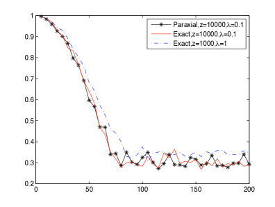
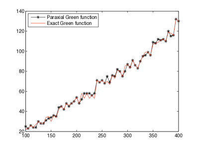
Figure 1. (Left) The red-solid and black-asterisk curves are, respectively, the coherence for the exact and paraxial sensing matrices for $z_{0}=10000,\lambda=0.1,n=100$ as a function of aperture. The blue-dashed curve is the coherence for the exact sensing matrix for $z_{0}=1000,\lambda=1,n=100$; (Right) the empirical, maximum number of recoverable sources with $|\sigma|=1$ v.s. the number $n$ of antennas for $A=100,\lambda=1$ by using the paraxial (black-asterisk) and exact (red-solid) sensing matrices.

To reduce the computational complexity of the compressed sensing step, we use an iterative scheme called Subspace Pursuit (SP) [9]. It has been shown to yield the BP solution under the RIP [9] (see Appendix A.

In the scattering simulation, we use the Foldy-Lax formulation accounting for all the multiple scattering effect [15]. Hence there are two mismatches (the paraxial approximation and the Born approximation) in the simulation.

In the left plot of Figure 2 the compressed sensing image with RM set-up is shown for $A=100$ and $n=20$. The size of the sensing matrix is $400\times 2500$ and $35$ targets are (nearly) exactly recovered. For comparison, the image obtained by the linear processor of the traditional matched field processing is shown on the right. In Appendix C, we outline the rudiments of matched field processing.

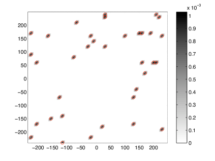
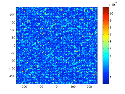
Figure 2. (Left) 35 scatterers are perfectly recovered by compressed sensing technique with $20$ antennas. The red circles represent the true locations of the targets. The plot on the right is produced by the conventional matched field processing.

In Figure 3 the numerically found maximum number of recoverable scatterers is depicted as a function of the number of antennas for $A=100$ and for both RM and SA imaging set-ups by using the paraxial and exact sensing matrices. Clearly, both curves are qualitatively consistent with the predictions (49) and (51).

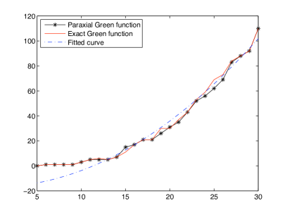
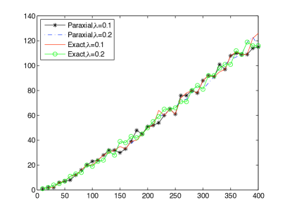
Figure 3. The empirical maximum number of recoverable scatterers (left for RM, right for SA) with $|\sigma|=0.001$ v.s. the number $n$ of antennas (or antenna locations) for $A=100$. The data for $n\in[10,30]$ in the RM plot is fitted with the parabola (blue-dashed curve): $-16.4950+0.1366*x^{2}$. The wavelength is $0.1$ for the RM case. The SA plot depicts the number of recoverable scatterers in four settings: paraxial sensing matrix with $\lambda=0.1$ (black-asterisk), paraxial sensing matrix with $\lambda=0.2$ (blue-dashed), exact sensing matrix with $\lambda=0.1$ (red-solid) and exact sensing matrix with $\lambda=0.2$ (green-circled)

6. Conclusions

In this paper, we have studied the imaging problem from the perspective of compressed sensing, in particular the idea that sufficient incoherence and sparsity guarantee uniqueness of the solution. Moreover, by adopting the target ensemble following [28] and the sensor ensemble, the maximum number of recoverable targets is proved to be at least proportional to the number of measurement data modulo a log-square factor with overwhelming probability.

We have analyzed three imaging settings: the inverse source, the inverse scattering with the response matrix and with the synthetic aperture. Important contributions of our analysis include the discoveries of the decoherence effect induced by random antenna locations and the threshold aperture defined by $\rho=1$ for source and RM imaging and $\rho=1/2$ for SA imaging where $\rho=\lambda z_{0}/(A\ell)$.

In this paper we have considered the localization of point targets and the determination of their amplitudes. A natural next step is to consider extended targets. However our approach does not extend in a straightforward manner to imaging of extended targets, as can be easily seen. Assume that we model an extended target approximately as an ensemble of point targets that are spaced very close together. Clearly, this requires the mesh size $\ell$ to be so small as to render $\rho\gg 1$. To apply our theorems would then require that the aperture and the number of antennas increase without bound. Clearly this is not a feasible way to image extended targets via compressed sensing. Therefore a somewhat different approach, on which we plan to report in our future work, is required for extended targets.

Appendix A Restricted isometry property (RIP)

A fundamental notion in compressed sensing under which BP yields the unique exact solution is the restrictive isometry property due to Candès and Tao [7]. Precisely, let the sparsity $s$ of the target vector be the number of nonzero components of $X$ and define the restricted isometry constant $\delta_{s}$ to be the smallest positive number such that the inequality

$$(1-\delta_{s})\|Z\|_{2}^{2}\leq\|\mathbf{A}Z\|_{2}^{2}\leq(1+\delta_{s})\|Z\|_{2}^{2}$$

holds for all $Z\in\mathbb{C}^{m}$ of sparsity at most $s$.

Now we state the fundamental result of the RIP approach.

Theorem 9.

[7] Suppose the true target vector $X$ has the sparsity at most $s$. Suppose the restricted isometry constant of $\mathbf{A}$ satisfies the inequality

(52) $$\delta_{3s}+3\delta_{4s}<2.$$

Then $X$ is the unique solution of BP.

Remark 6.

Greedy algorithms have significantly lower computational complexity than linear programming and have provable performance under various conditions. For example under the condition $\delta_{3s}<0.06$ the Subspace Pursuit (SP) algorithm is guaranteed to exactly recover $X$ via a finite number of iterations [9].

In this appendix we show that the sensing matrix for source inversion satisfies RIP. This can be readily seen by rewriting the paraxial Green function (3)

(53) $$G(\mathbf{r},{\mathbf{a}})={e^{i\omega z_{0}}\over 4\pi z_{0}}e^{i\omega(x^{2}+y^{2})/(2z_{0})}e^{-i\omega x\xi/z_{0}}e^{-i\omega y\eta/z_{0}}e^{i\omega(\xi^{2}+\eta^{2})/(2z_{0})},$$

for $\mathbf{r}=(x,y,z_{0}),{\mathbf{a}}=(\xi,\eta,0).$

Now the sensing matrix (5) can be written as the product of three matrices

$$\mathbf{A}=\mathbf{D}_{1}\mathbf{\Phi}\mathbf{D}_{2}$$

where

$$\mathbf{D}_{1}=\hbox{diag}(e^{i\omega(\xi_{j}^{2}+\eta_{j}^{2})/(2z_{0})}),\quad\mathbf{D}_{2}=\hbox{diag}(e^{i\omega(x_{l}^{2}+y^{2}_{l})/(2z_{0})})$$

are unitary and

$$\mathbf{\Phi}=n^{-1/2}\left[e^{-i\omega\xi_{j}x_{l}/z_{0}}e^{-i\omega\eta_{j}y_{l}/z_{0}}\right].$$

Assume without loss of generality that $x_{l}=y_{l}=l\ell,l=0,...,m-1$ and suppose that $(\xi_{j},\eta_{j}),j=1,...,n$ are independently and uniformly distributed in $[0,A]\times[0,A]$ with

(54) $${A\ell\over\lambda z_{0}}=1,$$

cf. (15).

The result essential for our problem is due to Rauhut [23].

Theorem 10.

[23] If

$${n\over\ln{n}}\geq Cs\ln^{2}{s}\ln{m}\ln{1\over\epsilon}$$

for $\epsilon\in(0,1)$ and some absolute constant $C$, then the restricted isometry condition (52) is satisfied with probability at least $1-\epsilon$.

See [5, 24] for similar results for sensors located in a particular discrete subset of $[0,A]\times[0,A]$.

Since $\mathbf{D}_{1}$ and $\mathbf{D}_{2}$ are diagonal and unitary, $\mathbf{A}$ satisfies (52) if and only if $\mathbf{\Phi}$ satisfies the same condition.

Theorem 11.

Let the sensor array be randomly drawn from the sensor ensemble satisfying (54). If

$${n\over\ln{n}}\geq Cs\ln^{2}{s}\ln{m}\ln{1\over\epsilon}$$

for $\epsilon\in(0,1)$ and some absolute constant $C$, then with probability at least $1-\epsilon$ all source amplitudes of sparsity less than $s$ can be uniquely determined from BP.

From the relationships (9), (10) it follows immediately that $\mathbf{A}^{\rm SA}$ also satisfies (52) if

(55) $${A\ell\over\lambda z_{0}}={1\over 2},$$

cf. (50).

Theorem 12.

Let the sensor array be randomly drawn from the sensor ensemble satisfying (55). If

$${n\over\ln{n}}\geq Cs\ln^{2}{s}\ln{m}\ln{1\over\epsilon}$$

for $\epsilon\in(0,1)$ and some absolute constant $C$, then with probability at least $1-\epsilon$ all scatter amplitudes of sparsity less than $s$ can be uniquely determined from BP.

The superiority of the RIP approach, if it works, over that of the incoherence taken in the main text of the paper, is that the uniqueness for BP is guaranteed for all targets of sparsity at most $s$ and the target ensemble needs not be introduced. Moreover, the stability of solution w.r.t. noise is guaranteed [6, 19]. However, Theorem 7 for the response matrix imaging does not seem amenable to the RIP approach.

Appendix B Proof of Theorem 1

Theorem 1 is an easy consequence from the following two theorems due to Tropp [28].

Proposition 2.

[28] Let $A$ be a $n\times m$ matrix with full rank. Let $\mathbf{A}_{s}$ be a submatrix generated by randomly selecting $s$ columns of $\mathbf{A}$. The condition

(56) $$6\left(p\mu^{2}s\ln{(1+s/2)}\right)^{1/2}+{s\over m}\|\mathbf{A}\|_{2}^{2}\leq{\alpha\over 2e^{1/4}},\quad p\geq 1$$

implies that

(57) $$\mathbb{P}\left(\|\mathbf{A}_{s}^{*}\mathbf{A}_{s}-\mathbf{I}_{s}\|_{2}<\alpha\right)\geq 1-\left({2\over s}\right)^{p}.$$

Proposition 3.

[28] Let $X$ be drawn from the target ensemble. If

(58) $$\mu^{2}s\leq\left(8\ln{m\over\epsilon}\right)^{-1},\quad\epsilon\in(0,1)$$

and if the least singular value

(59) $$\sigma_{\rm min}(\mathbf{A}_{s})\geq 2^{-1/2},\quad|S|=s$$

then $X$ is the unique solution of BP (L1), except with probability $2\epsilon$.

First of all, (13) and (14) together imply (56) and (58) with $\alpha=1/2$. Moreover, by Proposition 2 (59) holds with probability greater than or equal to the right hand side of (57). Hence we need only to derive the claimed bound for the probability of the event $E$ that $X$ is the unique solution of BP. This follows from the estimate

$$\mathbb{P}(E) \geq \mathbb{P}(E\big{|}\|\mathbf{A}_{s}^{*}\mathbf{A}_{s}-\mathbf{I}_{s}\|_{2}<2^{-1})\mathbb{P}(\|\mathbf{A}_{s}^{*}\mathbf{A}_{s}-\mathbf{I}_{s}\|_{2}<2^{-1})$$

$$\geq (1-2\epsilon)(1-(2/s)^{p})$$

$$\geq 1-2\epsilon-(2/s)^{p}.$$

Appendix C Matched field processing

Matched field processing (MFP) has been used extensively for source localization in underwater acoustics and is closely related to the matched filter in signal processing.

The conventional MFP uses the Bartlett processor with the ambiguity surface

(60) $$B(\mathbf{r})={{\mathbf{G}}^{*}(\mathbf{r})YY^{*}{\mathbf{G}}(\mathbf{r})\over\|{\mathbf{G}}(\mathbf{r})\|_{2}^{2}}$$

[25]. The Bartlett processor is motivated by the following optimization problem: Maximize the quantity

(61) $$W^{*}YY^{*}W$$

subject to the constraint:

$$W^{*}W=1.$$

The solution

$$W=Y/\|Y\|_{2}$$

is the weight vector for the matched filter. In the case of one point source of amplitude $\sigma_{1}$ located at $\mathbf{x}_{1}$,

$$Y=\sigma_{1}{\mathbf{G}}(\mathbf{r}_{1})$$

hence

(62) $$W={\sigma_{1}{\mathbf{G}}(\mathbf{r}_{1})\over|\sigma_{1}|\|{\mathbf{G}}(\mathbf{r}_{1})\|_{2}}.$$

Extending (62) to an arbitrary field point $\mathbf{r}$ by substituting $\mathbf{r}$ for $\mathbf{r}_{1}$ we obtain the Bartlett processor from (61).

In general, $Y$ is the $n$-dimensional measurement vector consisting the received signals of the array. For inverse scattering in the RM set-up, there are $n$ measurement vectors corresponding to $n$ probe signals. The ambiguity surface in this case is the sum of the $n$ ambiguity surfaces for the $n$ probe signals.

In contrast to the conventional matched field processor, the compressed sensing processor utilizing the $\ell^{1}$-minimization [6, 11] or various greedy algorithms [9, 21, 22, 26] are nonlinear.

References

• [1] A.B. Baggeroer, W.A. Kuperman and P.N. Mikhalevsky, ”An overview of matched field methods in ocean acoustics”, IEEE J. Oceanic Eng.18 (1993), 401-424.
• [2] B. Borden, Radar Imaging of Airborne Targets. Institute of Physics Publishing, Bristol, 1999.
• [3] M. Born and E. Wolf, Principles of Optics, 7-th edition, Cambridge University Press, 1999.
• [4] A.M. Bruckstein, D.L. Donoho and M. Elad, “From sparse solutions of systems of equations to sparse modeling of signals,” SIAM Rev. 51 (2009), 34-81.
• [5] E. Candés, J. Romberg and T. Tao, “Robust undertainty principles: Exact signal reconstruction from highly incomplete frequency information,” IEEE Trans. Inform. Theory 52 (2006), 489-509.
• [6] E.J. Candès, J. Romberg and T. Tao, “Stable signal recovery from incomplete and inaccurate measurements,” Commun. Pure Appl. Math. 59 (2006), 1207 23.
• [7] E. J. Candès and T. Tao, “ Decoding by linear programming,” IEEE Trans. Inform. Theory 51 (2005), 4203 4215.
• [8] J. C. Curlander and R.N. McDonough, Synthetic Aperture Radar: Systems and Signal Processing, Wiley-Intersience, 1991.
• [9] W. Dai and O. Milenkovic, “Subspace pursuit for compressive sensing: closing the gap between performance and complexity,” arXiv:0803.0811.
• [10] P. Delsarte, J. M. Goethals, and J. J. Seidel, Bounds for systems of lines and Jacobi poynomials, Philips Res. Repts. 30:3 pp. 91 105, 1975, issue in honour of C.J. Bouwkamp.
• [11] D. L. Donoho, “Compressed sensing,” IEEE Trans. Inform. Theory 52 (2006) 1289-1306.
• [12] D.L. Donoho and M. Elad, “Optimally sparse representation in general (nonorthogonal) dictionaries via $\ell^{1}$ minimization,” Proc. Nat. Acad. Sci. 100 (2003) 2197-2202.
• [13] D.L. Donoho, M. Elad and V.N. Temlyakov, “Stable recovery of sparse overcomplete representations in the presence of noise,” IEEE Trans. Inform. Theory 52 (2006) 6-18.
• [14] D.L. Donoho and X. Huo, “Uncertainty principle and ideal atomic decomposition, ” IEEE Trans. Inform. Theory 47 (2001), 2845-2862.
• [15] A.C. Fannjiang and P. Yan, “Multi-frequency imaging of multiple targets in Rician fading channels: stability and resolution,” Inverse Problems 23 (2007) 1801-1819.
• [16] A. Fannjiang, K. Solna and P. Yan, “Synthetic aperture imaging of multiple point targets in Rician fading media,” SIAM J. Imaging Sci.2 (2009), 344-366.
• [17] R. Gribonval and M. Nielsen, “Sparse representation in unions of bases,” IEEE Trans. Inform. Theory 49 (2003), 3320-3325.
• [18] M. Herman and T. Strohmer, “ High-resolution radar via compressed sensing,” to appear, IEEE Trans. Sign. Proc.
• [19] M. Herman and T. Strohmer, “General deviants: an analysis of perturbations in compressed sensing,” Preprint, Feb. 2009.
• [20] W. Hoeffding, “Probability inequalities for sums of bounded random variables”, J. Amer. Stat. Assoc. 58 (1963) 13 30.
• [21] D. Needell, J. A. Tropp, and R. Vershynin, “Greedy signal recovery review,” Proc. 42nd Asilomar Conference on Signals, Systems, and Computers, Pacific Grove, CA, Oct. 2008.
• [22] D. Needell and R. Vershynin, “Uniform uncertainty principle and signal recovery via regularized orthogonal matching pursuit”, Found. Comput. Math., DOI: 10.1007/s10208-008-9031-3.
• [23] H. Rauhut, “Stability results for random sampling of sparse trigonometric polynomials,” preprint, 2008.
• [24] M. Rudelson and R. Vershynin, “On sparse reconstruction from Fourier and Gaussian measurements,” Comm. Pure Appl. Math. 111 (2008) 1025-1045.
• [25] A. Tolstoy, Matched Field Processing in Underwater Acoustics, World Scientific, Singapore, 1993.
• [26] J.A. Tropp, “Greed is good: algorithmic results for sparse approximation,” IEEE Trans. Inform. Theory 50 (2004), 2231-2242.
• [27] J.A. Tropp, “ Just relax: convex programming methods for identifying sparse signals in noise,” IEEE Trans. Inform. Theory 52 (2006), 1030-1051. “Corrigendum” IEEE Trans. Inform. Theory (2008).
• [28] J.A. Tropp, “On the conditioning of random subdictionaries,” preprint, 2007.
• [29] H.C. van de Hulst, Light Scattering by Small Particles. Dover Publications, New York, 1981.
• [30] L. Welch, Lower bounds on the maximum cross-correlation of signals, IEEE Trans. on Information Theory, 20 (1974), pp. 397 399.