An Asymmetric Elastic Rod Model for DNA

Abstract

In this paper we consider the anharmonic corrections to the anisotropic elastic rod model for DNA. Our model accounts for the difference between the bending energies of positive and negative rolls, which comes from the asymmetric structure of the DNA molecule. We will show that the model can explain the high flexibility of DNA at small length scales, as well as kink formation at high deformation limit.

Characterizing the elastic behavior of DNA molecule is of crucial importance in understanding its biological functions. In recent years, single-molecule experiments such as DNA stretching and cyclization Smith et al. (1992); Crothers et al. (1992) have provided us with valuable information about the elasticity of long DNA molecules. The results of these experiments can be described by the elastic rod model (also called wormlike-chain model) Marko and Sigga (1995); Towles et al. . In this model it is assumed that the elastic energy is a harmonic function of the deformation Marko and Sigga (1994); Towles et al. . The elastic rod model is very successful in explaining the elastic behavior of the micron-size DNA molecules.

Recently, modern experimental techniques have made it possible to study the elasticity of DNA at nanometer length scale Cloutier and Widom (2004, 2005); Wiggins et al. (2006); Yuan et al. (2008). In these experiments it is observed that short DNA molecules are much more flexible than predicted by the elastic rod model. Several different models have been presented by now, that try to explain the origin of this discrepancy by considering the possibility of local DNA melting Yan and Marko (2004); Ranjith et al. (2005); Yuan et al. (2008); Destainville et al. , or the occurrence of kinks in the DNA structure Wiggins et al. (2005). Also Wiggins et al. have suggested an alternative form for the elastic energy Wiggins et al. (2006); Wiggins and Nelson (2006).

Since the DNA is not a symmetric molecule, the energy required to bend the DNA over its major groove is not equal to the energy required to bend it over its minor groove. The model which in introduced in this letter takes this difference into account. The effect of asymmetric structure of DNA on its elastic energy has been discussed previously by Marko and Siggia Marko and Sigga (1994), where they showed that there must be a coupling term between bend and twist in the harmonic elastic energy. We will discuss that the asymmetric structure of DNA can also be introduced as a correction to the harmonic elastic energy, which is of the third order. We shall show that our asymmetric elastic rod model can account for the high flexibility of short DNA molecules.

In the elastic rod model DNA is represented by a continuous inextensible rod. The curve which passes through the rod center determines the configuration of the DNA in three dimensional space. This curve is denoted by $\vec{r}$, and is parameterized by the arc length parameter $s$ (Figure 1). In addition, a local coordinate system with an orthonormal basis $\{\hat{d_{1}},\hat{d_{2}},\hat{d_{3}}\}$ is attached to each point of the rod. As depicted in Figure 1, $\hat{d_{3}}(s)$ is tangent to the curve $\vec{r}$ at each point, $\hat{d_{3}}(s)=\mathrm{d}\vec{r}/\mathrm{d}s$, $\hat{d_{1}}(s)$ is perpendicular to $\hat{d_{3}}(s)$ and points toward the major groove, and $\hat{d_{2}}(s)$ is defined as $\hat{d_{2}}(s)=\hat{d_{3}}(s)\times\hat{d_{1}}(s)$.

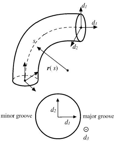
Figure 1: Parameterization of the elastic rod. The local frame $\{\hat{d_{1}},\hat{d_{2}},\hat{d_{3}}\}$ is attached to the rod.

These three orthogonal vectors uniquely determine the three dimensional configuration of DNA. From classical mechanics we have

$$\dot{\hat{d_{i}}}=\vec{\Omega}\times\hat{d}_{i}\quad\quad\quad i=1,2,3\,,$$ (1)

where the dot denotes the derivative with respect to $s$, and $\vec{\Omega}$ is called the spatial angular velocity. The components of $\vec{\Omega}$ in the local coordinate system are denoted by $\Omega_{1}$, $\Omega_{2}$, and $\Omega_{3}$. The elastic energy of an inextensible DNA in the most general form can then be written as

$$E=\int_{0}^{L}\mathcal{E}[\Omega_{1}(s),\Omega_{2}(s),\Omega_{3}(s)]\,\mathrm{d}s\,,$$ (2)

where $L$ is the total length of DNA. $\mathcal{E}(s)$ is the energy per unit length of DNA, i.e the energy density, at point $s$. For small deformations, the energy density can be written as a Taylor expansion about the lowest energy configuration Marko and Sigga (1994). For a DNA with no intrinsic curvature and a constant intrinsic twist $\omega_{0}$, the lowest energy configuration is given by $\vec{\Omega}_{0}=[0,0,\omega_{0}]^{\,T}$. Thus, at the lowest order, we arrive at a harmonic energy density in the form

$$\mathcal{E}_{\mathrm{harm}}[\Omega_{1},\Omega_{2},\Omega_{3}]=\frac{1}{2}k_{B}T\,\vec{\omega}^{\,T}\,\mathbf{Q}\,\,\vec{\omega}\,,$$ (3)

where $k_{B}$ is the Boltzmann constant, $T$ is the temperature, and $\vec{\omega}$ is defined by $\vec{\omega}=\vec{\Omega}-\vec{\Omega}_{0}$. $\mathbf{Q}$ is a $3\times 3$ symmetric matrix whose elements are the elastic constants of DNA Marko and Sigga (1995); Towles et al. ; Becker and Everaers (2007). Considering a short segment of DNA with the length $\mathrm{d}s$ at the point $s$, this segment has a symmetry under $180^{\circ}$ rotation about the local $\hat{d_{1}}$ axis at the point $s$. Thus the odd powers of $\Omega_{1}$ must not appear in the expansion of energy density, and the matrix $\mathbf{Q}$ has only four independent non-zero elements: $\mathbf{Q}_{11}$, $\mathbf{Q}_{22}$, $\mathbf{Q}_{33}$, and $\mathbf{Q}_{23}$. Therefore, the harmonic energy density can be written as Marko and Sigga (1994).

$$\mathcal{E}_{\mathrm{harm}}=\frac{1}{2}k_{B}T\big{[}A_{1}\,\Omega_{1}^{2}+A_{2}\,\Omega_{2}^{2}+C(\Omega_{3}-\omega_{0})^{2}$$

$$+2D\,\Omega_{2}(\Omega_{3}-\omega_{0})\big{]}.\qquad\qquad$$ (4)

The first two terms in equation (An Asymmetric Elastic Rod Model for DNA) correspond to the bending of DNA over its grooves (roll), and over its backbone (tilt), respectively. $A_{1}$ and $A_{2}$ are the corresponding bending constants. Since roll requires less energy than tilt C. R. Calladine and Horace R. Drew (1999); Lankas et al. (2000); Eslami-Mossallam and Ejtehadi (2008), one expects that $A_{2}<A_{1}$. The third term indicates the energy needed for twisting the DNA about its central axis, with the twist constant $C$. Finally, the fourth term accounts for the coupling between roll and twist Olson et al. (1998). Although the elastic constants of DNA may depend on the sequence Becker and Everaers (2007), in this paper we neglect sequence dependence, and assume that they are constant all along the DNA.

The existence of twist-roll coupling indicates that there is indeed a difference between bending over major groove (positive roll), and bending over minor groove (negative roll): For positive values of $D$, the DNA has a tendency to untwist when roll is positive, and to overtwist when roll is negative.
To account for the effect of asymmetry on the bending energy of DNA, we need a term in the energy density which is an odd function of $\Omega_{2}$, and does not depend on $\Omega_{1}$ or $\Omega_{3}$. There is no such term in the harmonic elastic energy, so we consider third-order terms in the expansion of energy density. The term proportional to $\Omega_{2}^{3}$ has the desired property. On the basis of some theoretical analysis Crick and Klug (1975), as well as experimental evidences Richmond and Davey (2003) and simulation studies Lankas et al. (2006), we assume that negative roll is more favorable than positive roll. Thus we write the third-order term in the form $+1/3!\,F^{2}\,\Omega_{2}^{3}$, where $F$ is a real parameter. (It must be noted that the main conclusion of the paper remains valid if positive roll is easier than negative roll. To account for this case, one can write the third-order term in the form $-1/3!\,F^{2}\,\Omega_{2}^{3}$.)
To keep the model as simple as possible, we neglect couplings in all orders, as well as higher-order corrections to the twist energy. So the only third-order term which enters in the model is $1/3!\,F^{2}\,\Omega_{2}^{3}$. Since the elastic energy must have a lower bound, we must keep the fourth-order correction to the roll energy, i. e. the term proportional to $\Omega_{2}^{4}$, in the model. For consistency of the model, we also keep the corresponding fourth-order correction to the tilt energy. Since the anisotropy in bending energy is accounted for in the second order, to reduce the model free parameters, we write the fourth-order terms in the form $1/4!\,G^{3}(\Omega_{1}^{4}+\Omega_{2}^{4})$, with $G$ real and positive. Adding third-order and fourth-order terms to the harmonic energy density, we obtain the asymmetric elastic rod model which is given by

$$\mathcal{E}_{\mathrm{asym}}=\!k_{B}T\Big{[}\frac{1}{2}A_{1}\,\Omega_{1}^{2}+\frac{1}{2}A_{2}\,\Omega_{2}^{2}+\frac{1}{2}C(\Omega_{3}-\omega_{0})^{2}$$

$$+\,\frac{1}{3\,!}\,F^{\,2}\,\Omega_{2}^{3}+\frac{1}{4\,!}\,G^{\,3}(\Omega_{1}^{4}+\Omega_{2}^{4})\Big{]}.$$

This model accounts for the asymmetry between positive and negative rolls, as well as the difference in the energies of roll and tilt. Since there is no coupling term in the model, roll, tilt, and twist can be regarded as independent deformations, and the energy density can be decompose into three separate terms

$$\mathcal{E}_{\mathrm{asym}}[\Omega_{1},\Omega_{2},\Omega_{3}]=\mathcal{E}_{1}[\Omega_{1}]+\mathcal{E}_{2}[\Omega_{2}]+\mathcal{E}_{3}[\Omega_{3}]\,,$$ (6)

where

$$\mathcal{E}_{1}=k_{B}T\Big{[}\frac{1}{2}A_{1}\,\Omega_{1}^{2}+\frac{1}{4\,!}\,G^{\,3}\,\Omega_{1}^{4}\Big{]},\qquad\qquad\qquad$$ (7)

$$\mathcal{E}_{2}=k_{B}T\Big{[}\frac{1}{2}A_{2}\,\Omega_{2}^{2}+\,\frac{1}{3\,!}\,F^{\,2}\,\Omega_{2}^{3}+\frac{1}{4\,!}\,G^{\,3}\,\Omega_{2}^{4}\Big{]},\,\,$$ (8)

$$\mathcal{E}_{3}=\frac{1}{2}k_{B}T\,C(\Omega_{3}-\omega_{0})^{2}\,.\qquad\qquad\qquad\qquad\quad$$ (9)

Depending on the values of $A_{2}$, $F$ and $G$, $\mathcal{E}_{2}$ can take three different forms (see Figure 2). For small values of $F$, $\mathcal{E}_{2}$ has only one minimum at $\Omega_{2}=0$ and its curvature is always positive. For $F>(2\,A_{2}\,G^{\,3})^{1/4}$ the curvature of $\mathcal{E}_{2}$ can change sign and there are two inflection points. For given $A_{2}$ and $G$ there exists an upper bound $F_{c}=(8/3\,\,A_{2}\,G^{\,3})^{1/4}$, beyond which $\mathcal{E}_{2}$ has two minima: one at $\Omega_{2}=0$ and the other one at a negative $\Omega_{2}$. In this case DNA has two stable configurations, and there is always a barrier between them. However, one expects that the barrier is not large compared to $k_{B}T$ for a real DNA.

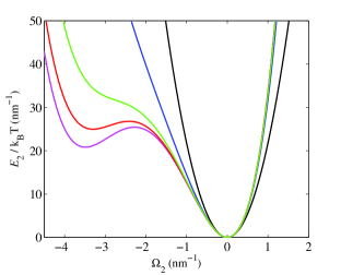
Figure 2: (Color online) $\mathcal{E}_{2}$ as a function of $\Omega_{2}$ for $A_{2}=43.50\,\mathrm{nm}$ and different values of $F$ and $G$. Black: $F=G=0$. Blue: $G=3.20\,\mathrm{nm}$ and $F=7.20\,\mathrm{nm}$, $\mathcal{E}_{2}$ has one minimum and its curvature is positive every where. Green: $G=3.20\,\mathrm{nm}$ and $F=7.80\,\mathrm{nm}$, $\mathcal{E}_{2}$ has two inflection points and one minimum. Red: $G=3.20\,\mathrm{nm}$ and $F=7.90\,\mathrm{nm}$, $\mathcal{E}_{2}$ has two minima. Magenta: $G=3.20\,\mathrm{nm}$ and $F=7.94\,\mathrm{nm}$. Note that a change of $0.04\,\mathrm{nm}$ in $F$ results in a change of about $1\,k_{B}T/l_{0}$ in $\mathcal{E}_{2}$ in the vicinity of the second minimum.

To study the elastic behavior of DNA in the asymmetric elastic rod model, we calculate the distribution function $P(\theta)$, the probability that the DNA bends into an angle $\theta$. We use a Monte Carlo simulation to calculate $P(\theta)$. In this simulation we discretize each chain into separate segments of length $l_{0}=0.34\,\mathrm{nm}$, equal to the base-pair separation in DNA. The orientation of each segment is then determined by a vector $\vec{\Theta}$, where $|\vec{\Theta}|$ determines the rotation angle of the local coordinate system with respect to the laboratory coordinate system, and the direction of $\vec{\Theta}$ indicates the normal to the plane of rotation. The special angular velocity is related to $\vec{\Theta}$ as $\vec{\Omega}=\vec{\Theta}/l_{0}$. In each Monte Carlo move, we randomly choose a segment along the chain, and for that segment we change the vector $\vec{\Theta}$ by $\Delta\vec{\Theta}$. The direction of $\Delta\vec{\Theta}$ is random, and its magnitude is chosen randomly in the interval $[0\,,\,\Theta_{0}]$. $\Theta_{0}$ is chosen so that the accept ratio is about $0.5$. We do not include the self avoiding in the simulation, since the probability of self crossing is small for the short simulated DNA molecules.

Recently, Wiggins et al. have used atomic force microscopy to measure distribution of the bending angle of short DNA molecules Wiggins et al. (2006). Although the DNA molecules in Wiggins et al. experiment has the characteristic properties of two dimensional polymers Wiggins et al. (2006), to simulate the experiment we do not confine the DNA completely in a plane. The reason is that the minimum energy configuration of an anisotropic DNA is not plannar, although the deviation from a plannar configuration is negligible Kehrbaum and Maddocks (2000). It is known in the anisotropic harmonic elastic rod model, that the effective bending constant of long DNA molecules in three dimensions is equal to the harmonic average of $A_{1}$ and $A_{2}$ Eslami-Mossallam and Ejtehadi (2008); Becker and Everaers (2007); Lankas et al. (2000), $A_{\mathrm{eff}}=\left[1/2\left(1/A_{1}+1/A_{2}\right)\right]^{-1}$, while in the two dimensions the effective bending constant is given by $A_{\mathrm{eff}}^{2D}=\sqrt{A_{1}\,A_{2}}$ Bijani et al. . Since $A_{\mathrm{eff}}^{2D}$ is always greater than $A_{\mathrm{eff}}$, confining the DNA in a plane costs energy. For this reason, we allow the DNA to come out of the plane by $0.3\,\mathrm{nm}$, which is seven times smaller than DNA diameter and lies in the range of atomic length scales.

Following other studies Towles et al. ; Moroz and Nelson (1998), we assume $A_{1}=2\,A_{2}$, $C=100\,\mathrm{nm}$, and $\omega_{0}=1.8\,\mathrm{nm^{-1}}$. The values of $A_{2}$, $F$ and $G$ are then determined by fitting the theoretical results to the experimental data of Wiggins et al., with the constrain that the persistence length of the DNA is $54\,\mathrm{nm}$ Wiggins et al. (2006). Figure 3 shows a good fit to the experimental data, which corresponds to $A_{2}=43.50\,\mathrm{nm}$ $G=3.20\,\mathrm{nm}$ $F=7.90\,\mathrm{nm}$. The predictions of isotropic-harmonic elastic rod model are also shown in the Figure. We report the values of the fitting parameter with three significant digits. The reason is that $\mathcal{E}_{2}$ is very sensitive to the changes of the parameters, specially when it has two minima. In fact, a change in the order of $10^{-2}\,\mathrm{nm}$ in these parameters may results in a change in $\mathcal{E}_{2}$ in the order of $1\,k_{B}T/\l_{0}$ (see Figure 2), and therefore can significantly affect the elastic behavior of DNA. We must note here that the ratio $A_{1}/A_{2}$ is also relevant to the fitting procedure. However, one can obtain equally good fits for different values of $A_{1}/A_{2}$.

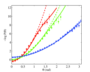
Figure 3: (Color online) $-\log P(\theta)$ as a function of $\theta$, for $L=5\,\mathrm{nm}$ (red), $L=10\,\mathrm{nm}$ (green), and $L=30\,\mathrm{nm}$ (blue). Dots show the experimental data of Wiggins et al. Wiggins et al. (2006). Curves show the theoretical results. Dashed curves: isotropic harmonic elastic rod model, with $A_{1}=A_{2}=54\,\mathrm{nm}$, and $F=G=0$. Solid curves: $A_{1}=87.00\,\mathrm{nm}$, $A_{2}=43.50\,\mathrm{nm}$ $F=7.90\,\mathrm{nm}$, and $G=3.20\,\mathrm{nm}$.

The functional form of $\mathcal{E}_{2}$ for $A_{2}=43.50\,\mathrm{nm}$, $F=7.90\,\mathrm{nm}$ and $G=3.20\,\mathrm{nm}$ is shown in Figure 2, which has two minima. The second minimum occurs at $\Omega_{2}=-3.3\,\mathrm{nm}^{-1}$ which corresponds to a $-64^{\circ}$ roll between adjacent base pairs. Thus, the existence of a second minimum can lead to the formation of kinks in the minor groove direction in a tightly bent DNA. As can be seen in Figure 3, both in the experiment and our model, $-\log P(\theta)$ deviates from the harmonic model at large bending angles. Continuing the graphs in our model, they arrive to an approximately linear regime. This linear behavior is a signature of kink formation. Both the slope of the line, and the crossover point are related to the values of $F$ and $G$.
The possibility of kink formation in the DNA structure has been considered previously by other authors. It was firstly mentioned by Crick and Klug, who proposed an atomistic structure for a kinked DNA Crick and Klug (1975). They suggest that DNA can be kink most easily toward the minor groove. Nelson, Wiggins, and Phillips have presented a simple model for kinkable elastic rods Wiggins et al. (2005), in which the kinks are completely flexible, and can be formed in any direction with equal probability. Their model can explain the high cyclization probability of short DNA molecules Cloutier and Widom (2004, 2005). The linear behavior is also observed in their model Wiggins et al. (2005), but the slope of the line is always zero. In a recent experiment, Du et al. proved the existence of kinks in DNA minicircles of 64-65 bp Du et al. (2008). Molecular dynamics simulations on a 94 bp minicircle Lankas et al. (2006) also show that kinks are formed, with the same structure predicted by Crick and Klug. Similar kinks in the direction of minor groove have been observed in the structure of nucleosomal DNA Richmond and Davey (2003).
Kinks are also observed in the crystal structures of non-histone protein-DNA complexes Dickerson (1998); Olson et al. (1998). In these complexes, DNA has a clear tendency to kink in the major groove direction. Du et al. have found the distribution function $P(\theta)$ for a base-pair step in these complexes Du et al. (2005). Although it is contradictory to our primary assumption, that kinks are formed toward the major groove, the asymmetric elastic rod model can be fitted to the Du et al. data by writing the third-order term in the form $-1/3!\,F^{2}\,\Omega_{2}^{3}$, and choosing $F=8.86\,\mathrm{nm}$ and $G=3.83\,\mathrm{nm}$. We found that the model with these values of $F$ and $G$ can not explain the experimental data of Wiggins et al.. This shows that the statistical property of DNA in the protein-DNA complexes certainly differs from the free DNA. This difference is probably due to the interaction of proteins with DNA, which can alter the DNA conformation dramatically, and leads to different effective elastic constants.

In this paper, we presented a generalization of the anisotropic elastic rod model, assuming that the energies of positive and negative rolls are different as a result of the asymmetric structure of DNA. We showed that this model can explain the elastic behavior of short DNA molecules. We also showed that this model allows the formation of kinks in the DNA structure when the DNA is tightly bent. The kinks always form in one of the groove directions, as suggested by other studies.