Counting Complex Disordered States by Efficient Pattern Matching:
Chromatic Polynomials and Potts Partition Functions

Abstract

Counting problems, determining the number of possible states of a large system under certain constraints, play an important role in many areas of science. They naturally arise for complex disordered systems in physics and chemistry, in mathematical graph theory, and in computer science. Counting problems, however, are among the hardest problems to access computationally. Here we suggest a novel method to access a benchmark counting problem, finding chromatic polynomials of graphs. We develop a vertex-oriented symbolic pattern matching algorithm that exploits the equivalence between the chromatic polynomial and the zero-temperature partition function of the Potts antiferromagnet on the same graph. Implementing this bottom-up algorithm using appropriate computer algebra, the new method outperforms standard top-down methods by several orders of magnitude, already for moderately sized graphs. As a first application we compute chromatic polynomials of samples of the simple cubic lattice, for the first time computationally accessing three-dimensional lattices of physical relevance. The method offers straightforward generalizations to several other counting problems.

Given a set of different colors, in how many ways can one color the vertices of a graph such that no two adjacent vertices have the same color? The answer to this question is provided by the chromatic polynomial of a graph Birkhoff ; Read , which gives the number of possible colorings as a function of the number $q$ of colors available. It is a polynomial in $q$ of degree $N$, the number of vertices of the graph. The chromatic polynomial is closely related to other graph invariants e.g. to the reliability and flow polynomials of a network or graph (functions that characterize its communication capabilities) and to the Tutte polynomial. These are of widespread interest in graph theory and computer science and pose similar hard counting problems.

The chromatic polynomial is also of direct relevance to statistical physics as it is equivalent to the zero-temperature partition function of the Potts antiferromagnet Potts ; Wu : The Potts model Potts constitutes a paradigmatic characterization of systems of interacting electromagnetic moments or spins, where each spin can be in one out of $q\geq 2$ states; it thus generalizes the Ising model where $q=2$. For antiferromagnetic interactions, neighboring spins tend to disalign such that at zero temperature, the partition function of the Potts antiferromagnet counts the number of ground states of a spin system just as the chromatic polynomial counts the number of proper colorings of the same graph. For sufficiently large $q$ there are many system configurations in which all pairwise interaction energies are minimized at zero temperature. Indeed, these systems exhibit a large number of disordered ground states that is exponentially increasing with system size. Thus the Potts model exhibits positive ground state entropy, an exception to the third law of thermodynamics. Experimentally, complex disordered ground states and related residual entropy at low temperatures have been observed in various systems Pauling ; Parsonage ; Ramirez ; Broholm ; Wills ; Fennel .

Although there are several analytical approaches to find chromatic polynomials for families of graphs and to bound their values BiggsMatrixMethod ; Birkhoff ; Potts ; SalasShrock64:011111 ; SokalAnalytics ; SokalAnalytics2001 ; Wu ; Read ; Jacobsen ; Rocek ; SalasSokal , there is no closed form solution to this counting problem for general graphs. Algorithmically it is hard to compute the chromatic polynomial, because the computation time in general increases exponentially with the number of edges in the graph HardComputation . It also strongly depends on the structure of the graph and rapidly increases with the graph’s size, and the degrees of its vertices, cf. MezardScience ; WeigtMuseum ; HartmannBook . Therefore, most studies on chromatic polynomials up to date have focused on small graphs and families of graphs of simple structure and low vertex degrees, e.g. two-dimensional lattice graphs SalasSokal ; Jacobsen ; Rocek (an interesting recent attempt to analytically study simple cubic lattices considered strips with reduced degrees SalasShrock64:011111 ). In fact, it is not at all straightforward to computationally access larger graphs with more involved structure, including physically relevant three-dimensional lattice graphs. Finding the chromatic polynomial of a graph thus constitutes a challenging, computationally hard problem of statistical physics, graph theory and computer science (cf. HardComputation ; HartmannBook ).

Below we present a novel, efficient method to compute chromatic polynomials of larger structured graphs. Representing a chromatic polynomial as a zero temperature partition function of the Potts antiferromagnet we transform the computation into a local and vertex-oriented, ordered pattern matching problem which we then implement using appropriate computer algebra. In contrast to conventional top-down methods that represent and process the entire graph (and many modified copies thereof) from the very beginning, the new method presented here works through the graph bottom-up and thus processes comparatively small local parts of the graph only.

Consider a graph $G$ that is defined by a set of $N$ vertices $i\in V=\{1,\ldots,N\}$ and a set of $M:=|E|$ edges $\{i,j\}\in E$, each edge joining two vertices $i$ and $j$ which are then called adjacent or neighboring. This graph is said to be (properly) $q$-colored if every vertex is given one out of $q$ colors $\{1,2,\ldots,q\}$ such that every two adjacent vertices have different colors. The number of $q$-colorings of a graph $G$ is expressed by its chromatic polynomial $P(G,q)$, a polynomial in $q$ of order $N$ Read .

The deletion-contraction theorem of graph theory Read suggests a simple algorithm to compute the chromatic polynomial of a given graph recursively. In principle, this algorithm works for arbitrary graphs and is therefore, with certain improvements, implemented in general-purpose computer algebra systems such as Mathematica Mathematica ; SkienaOriginal ; Pemmaraju and Maple Maple (cf. also Niejenhuis_et_al ; ReadWaterloo ). However, applying the theorem recursively the chromatic polynomial of exponentially many graphs must be found, the (weighted) sum of which yields the chromatic polynomial of the original graph. This reflects how hard the problem is algorithmically and severely restricts the applicability of computational methods, in particular if they employ standard top-down processing.

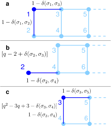
Figure 1: The bottom-up, local and vertex-oriented nature of the algorithm. Sequential processing of edges (dark) adjacent to vertices (a) $i=1$, (b) $i=2$, and (c) $i=3$. The remainder graph (light) is not affected when processing vertex $i$. Partial partition functions $z_{i-1}$ computed so far (before each vertex step $i$) are shown in square brackets.

We now describe our novel algorithm. It is based on the antiferromagnetic ($J<0)$ Potts model Potts ; Wu with Hamiltonian

$$H(\boldsymbol{\sigma})=-J\sum_{\{i,j\}\in E}\delta_{\sigma_{i}\sigma_{j}}$$ (1)

giving the total energy of the system in state $\boldsymbol{\sigma}=(\sigma_{1},\ldots,\sigma_{N})$. Here individual spins $\sigma_{i}$ can assume $q$ different values $\sigma_{i}\in\{1,\ldots,q\}$, generalizing he Ising model ($q=2$) Ising . Two spins $\sigma_{i}$ and $\sigma_{j}$ on the graph $G$ interact if and only if they are neighboring, $\{i,j\}\in E$, and in the same state, $\sigma_{i}=\sigma_{j}$, i.e. the Kronecker-delta is $\delta_{\sigma_{i}\sigma_{j}}=1$ (otherwise, for any pair $\sigma_{i}\neq\sigma_{j}$, it is $\delta_{\sigma_{i}\sigma_{j}}=0$). Thus the total interaction energy is minized if all pairs of neighboring spins are in different states.

The partition function $Z(G,q,T)=\sum_{\boldsymbol{\sigma}}\exp(-\beta H(\boldsymbol{\sigma}))$ at positive temperature $T=(k_{\textrm{B}}\beta)^{-1}$, where $k_{\textrm{B}}$ is the Boltzmann constant, can be represented as

$$Z(G,q,T)=\sum_{\boldsymbol{\sigma}}\prod_{\{i,j\}\in E}(1+v\delta_{\sigma_{i}\sigma_{j}})$$ (2)

where $v=\exp(\beta J)-1\in(-1,0].$ In the limit $T\rightarrow 0$ (implying $\beta J\rightarrow-\infty$ and thus $v\rightarrow-1$) this partition function counts the number of ways of arranging the spins $\mathbf{\sigma}$ such that no two adjacent spins are in the same state. Thus the zero temperature partition function (2) exactly equals Wu the chromatic polynomial

$$P(G,q)=\lim_{T\rightarrow 0}Z(G,q,T)$$ (3)

on the same graph $G$ leading to the representation Wu ; SokalAnalytics

$$P(G,q)=\sum_{\sigma_{1}=1}^{q}\cdots\sum_{\sigma_{N}=1}^{q}\prod_{\{i,j\}\in E}(1-\delta_{\sigma_{i}\sigma_{j}})$$ (4)

of the chromatic polynomial in terms of sums over products of Kronecker-deltas.

The algorithm exploits this representation by expanding the products in (4) and symbolically evaluating the right hand side vertex by vertex (cf. Fig. 1), considering each individual sum $\sum_{\sigma_{k}}$ as an operator. This operator interpretation relies on a recently studied algebraic structure of expressions containing Kronecker-deltas Kozen . Here such an operator has the simple actions

$$\sum_{\sigma_{k}}1=q,$$ (5)

$$\sum_{\sigma_{k}}\delta_{\sigma_{k}\sigma_{j_{1}}}=1,$$ (6)

$$\sum_{\sigma_{k}}\delta_{\sigma_{k}\sigma_{j_{1}}}\delta_{\sigma_{k}\sigma_{j_{2}}}=\delta_{\sigma_{j_{1}}\sigma_{j_{2}}}\,,$$ (7)

and for an arbitrary number $r\in\mathbb{N}_{0}$ of factors,

$$\sum_{\sigma_{k}}\delta_{\sigma_{k}\sigma_{j_{1}}}\cdots\delta_{\sigma_{k}\sigma_{j_{r}}}=\delta_{\sigma_{j_{1}}\sigma_{j_{2}}}\cdots\delta_{\sigma_{j_{r-1}}\sigma_{j_{r}}}$$ (8)

if the $j_{\rho}$, $\rho\in\{1,\ldots,r\}$, are pairwise distinct and all $j_{\rho}\neq k$.

For illustration consider the chromatic polynomial

$$P(G,q)=\sum_{\sigma_{3}=1}^{q}\sum_{\sigma_{2}=1}^{q}\sum_{\sigma_{1}=1}^{q}(1-\delta_{\sigma_{1}\sigma_{2}})(1-\delta_{\sigma_{1}\sigma_{3}})(1-\delta_{\sigma_{2}\sigma_{3}})$$ (9)

of a triangular (complete) graph comprised of $N=3$ vertices and $M=3$ edges. We start at vertex $i=1$ by expanding the relevant product

$$p_{1} =(1-\delta_{\sigma_{1}\sigma_{2}})(1-\delta_{\sigma_{1}\sigma_{3}})$$ (10)

$$=1-\delta_{\sigma_{1}\sigma_{2}}-\delta_{\sigma_{1}\sigma_{3}}+\delta_{\sigma_{1}\sigma_{2}}\delta_{\sigma_{1}\sigma_{3}}$$ (11)

that is comprised of all factors that contain $\sigma_{1}$. (We note that already Birkhoff Birkhoff in 1912 used closely related expansions to theoretically derive an alternative representation of chromatic polynomials.) Symbolically applying the above replacement rules (8) yields a “partial partition function”

$$z_{1} = \sum_{\sigma_{1}=1}^{q}p_{1}$$ (12)

$$= q-2+\delta_{\sigma_{2}\sigma_{3}}\,,$$ (13)

and thus $P(G,q)=\sum_{\sigma_{3}=1}^{q}\sum_{\sigma_{2}=1}^{q}z_{1}(1-\delta_{\sigma_{2}\sigma_{3}})$. Proceeding with the vertices $i=2$ and $i=3$ in a similar fashion, we obtain $p_{2}=(q-2+\delta_{\sigma_{2}\sigma_{3}})(1-\delta_{\sigma_{2}\sigma_{3}})$, $z_{2}=\sum_{\sigma_{2}=1}^{q}p_{2}=(q-1)(q-2)$, $p_{3}=z_{2}$, and reduce the chromatic polynomial to the final result $P(G,q)=z_{3}=\sum_{\sigma_{3}=1}^{q}p_{3}=q(q-1)(q-2)$, successively.

For a general graph $G$ on $N$ vertices, the algorithm is analogous to the example. First define $z_{0}=1$. Then, passing through the vertices from $i=1$ sequentially up to $i=N$,

1. construct and expand $p_{i}=z_{i-1}\prod_{\{i,j\}\in E}(1-\delta_{\sigma_{i}\sigma_{j}})$ where the product is over all edges incident to $i$ that have not been considered before, i.e. $j>i$;

2. symbolically evaluate the sum $z_{i}=\sum_{\sigma_{i}}p_{i}$ applying the simple rules (5)-(8) given above.

These operations are local and vertex oriented in the sense that they jointly consider all edges $\{i,j\}$ incident to an individual vertex $i$ at any one time. A major advantage of this bottom-up algorithm is that all edges that are not currently processed are kept outside the computations until they are needed, quite in contrast to standard top-down deletion-contraction algorithms. If a graph $G$ has a layered structure,

$$G=\bigcup_{\nu}H_{\nu}$$ (14)

with layers $H_{\nu}$, constituting samples of periodic lattices or aperiodic graphs, the vertices $i$ are selected (i.e. numbered) layer by layer such that the operations only affect a particularly small portion of the graph at once (Fig. 1). These graphs have bounded tree widths, cf. Andrzejak ; Noble . More generally, vertices are numbered appropriately beforehand, for instance, using minimal band width of the graph as a heuristic criterion WestBandWidth .

The computation of the chromatic polynomial has been reduced to a process of alternating expansion of expressions and symbolically replacing terms in an appropriate order. In the language of computer science, these operations are represented as the expanding, matching, and sorting of patterns, making the algorithm suitable for computer algebra programs optimized for pattern matching.

To fully exploit the capabilities of this algorithm, we implemented it using the language Form Form ; Vermaseren which is specialized to large scale symbolic manipulation problems and as such a successful standard tool for, e.g., Feynman diagram evaluation in precision high-energy physics Laporta ; Misiak .

A practically relevant measure for the speed of our method is the total CPU time $t$ it needs for a specific calculation. For hard counting problem, one generally expects an exponential increase $t\approx A\exp(\alpha m)\,$ with the size $m\gg 1$ of the problem, here defined as the number $m=M$ of edges for chromatic polynomials of general graphs. For graphs with bounded tree width Andrzejak ; Noble the solution time of the counting problem typically only grows exponentially with the width of the graph, i.e. in the square of the number of vertices in the subgraphs $H_{\nu}$. The factor $\alpha$ in the exponent determines the scaling of the computational time with problem size and measures the efficiency of the algorithm, whereas the prefactor $A$ fixes the absolute time needed and depends, among others, on the software environment and hardware used.

Figure 2: Computation time $t$ (in ms) for square lattice samples of sizes $2\times n$ (main panel) and $n\times n$ (inset) increases with the number of edges $M$ of the graph. The new method ($\bullet$) drastically outperforms standard methods used in Mathematica ($\bigcirc$) and Maple ($\square$), both with respect to the scaling of the algorithm (quantified by the local slope) and the absolute effectiveness (quantified by the absolute times needed), even for moderately sized graphs.

To compare our method to existing ones, we first computed chromatic polynomials of samples of the two-dimensional square lattice with free boundary conditions ($2\times n$ strips that have $M=3n-2$ edges and $n\times n$ patches that have $M=2n(n-1)$ edges). The total computation times $t$ have been measured as a function of $M$ for the new method as well as for the standard methods used in Mathematica Mathematica ; SkienaOriginal and Maple Maple , respectively. Figure 3 shows that the scaling $\alpha$ of the algorithm (given by the local slope of the data points in the logarithmic plot) of our new method is markedly better than the one found for the standard deletion-contraction methods. This implies that the new method outperforms these standard computational methods in the absolute computation time by several orders of magnitude already for moderately sized graphs (e.g. about six orders of magnitude for $n=10$ i.e. $M=28)$. With increasing graph size, the advantages of our method become more pronounced. For example, for the $2\times 100$ strip of the square lattice ($M=298$ edges) the pattern matching method needs a computation time of the order of $t\approx 2s$ whereas extrapolation of the data shown in Fig. 3 indicates that the same problem is not computationally accessible using the standard deletion-contraction methods implemented in Mathematica.

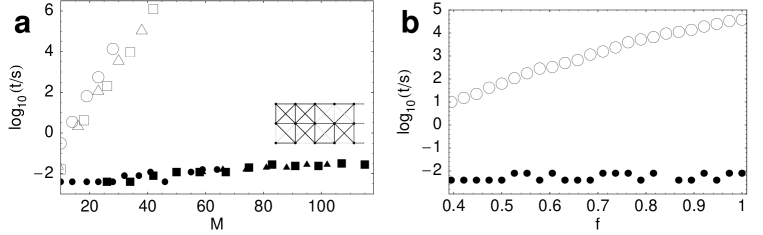
Figure 3: Computation time $t$ (in ms) for randomly edge-diluted square lattice samples with next nearest neighbor (nnn) interactions (displayed as a cartoon inset in panel (a)). The new method (filled symbols) strongly outperforms standard deletion-contraction method (Mathematica, open symbols). (a) Computation time vs. the actual total number $M$ of edges for samples of $3\times n$ vertices where each original edge has been deleted independently with probability $p=0.1$ (circles) $p=0.2$ (triangles) and $p=0.5$ (squares). (b) Computation time vs. the fraction $f$ of edges present. Edges are sequentially randomly removed independently, starting from an undiluted $3\times 5$ square lattice graph ($f=1)$ with nnn interactions; the graph is diluted until before it becomes disconnected below $f\approx 0.4$. Whereas the computation times using the new method are still at fluctuation level ($t<10^{-2}s)$, standard methods take at factor of $10^{3}$ to $10^{7}$ longer.

Second, in contrast to transfer matrix or other analytical recurrence methods SokalAnalytics ; SokalAnalytics2001 ; SalasSokal , the above method also works in a simple way for graphs with non-identical subgraphs $H_{\nu}$, such as randomly diluted lattices. The same comparison for randomly diluted $3\times n$ square lattice samples with next-nearest neighbor interactions (Fig. 3) confirms the pronounced outperformance and moreover illustrates the general applicability of our method, also compared to recursive analytical methods.

As a first application to an open hard counting problem, we now turn to three-dimensional lattices of direct physical relevance. First, we consider $n\times n\times n$ samples of the simple cubic lattice with free boundary conditions, which have $N=n^{3}$ vertices and $M=3n^{2}(n-1)$ edges. We found chromatic polynomials up to $n=4$ ($N=64$, $M=144$). A representation of the chromatic polynomial $P(G,q)$ in terms of its $N$ complex zeroes $q_{1},\ldots,q_{N}$ is shown in Fig. 4a for $n=3$ and $n=4$. We further consider simple cubic lattice strips that extend in the diagonal (111) direction with periodic boundaries in the two other (transverse) directions. This keeps the number of vertices within one layer low at the same time allowing for a large number $N_{c}$ of vertices with the same degree (equal to six) as vertices in the infinite lattice, a fact that is heuristically known to be essential for a rapid convergence towards the thermodynamic limit ($N,M\rightarrow\infty$). The largest three-dimensional sample graphs shown in Figure 4b have $N=384$ vertices, $M=1128$ edges and a fraction $N_{c}/N=368/384\approx 0.96$ of vertices with correct degree, (as compared to $N_{c}/N=8/64\approx 0.13$ for the $4\times 4\times 4$ sample extending along the Cartesian axes and to $N_{c}=0$ for previous attempts to address three-dimensional lattices). The computation time was approximately 11 hours on a single Linux machine with an Intel Pentium 4, 2.8 GHz-32 bit processor.

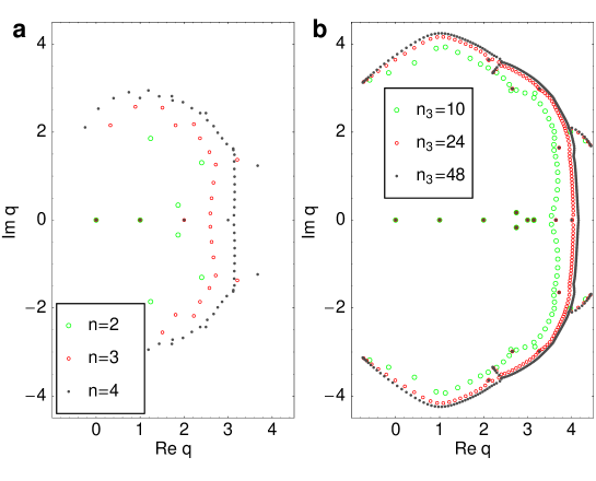
Figure 4: Complex zeroes representing chromatic polynomials of samples of the simple cubic lattice (a) $n\times n\times n$ Cartesian samples with free boundary conditions, and (b) $2\times 4\times n_{3}$ diagonal samples with periodic transverse boundary conditions, with up to $M=1128$ edges.

In summary we have presented a novel method to calculate chromatic polynomials of graphs. Using the partition function representation, it proceeds vertex by vertex employing an a priori reduction to local operations only and is thus particularly suited for graphs exhibiting a layered structure. The method combines a symbolic bottom-up algorithm, which is based on systematic term-wise expansion and pattern matching, with an appropriate computer algebra program Form ; Vermaseren . Our method is applicable to general types of graphs, including graphs with bounded and unbounded tree widths as well as randomized graphs. We demonstrated by several sets of examples that it drastically outperforms existing standard methods for all these types of graphs. As a practical application, we computed chromatic polynomials for samples of the simple cubic lattice, for the first time computationally accessing three-dimensional lattices of physical relevance.

Since the main ideas underlying our method are simple to apply, they may be generalized in a straightforward way and also be transferred to other challenging counting problems. Among others, one may compute quantitative measures relevant in computer science that give information about the communication capabilities of a network, such as (i) the flow polynomial and (ii) the reliability polynomial FlowPolynomials ; ReliabilityPolynomials . It is equally possible to determine (iii) ferromagnetic and (iv) positive temperature partition functions of statistical physics ChangposT ; Haeggkvist ; Chen and, equivalently, (v) the Tutte polynomial (of two variables $q$ and $v$, cf. Eq. 2), valuations of which directly result in the number of spanning subgraphs, the number of spanning trees, and other invariants of a graph SokalAnalytics ; SokalAnalytics2001 . Of course, applications in graph theory may include studies of families of graphs where computational results seemed impossible so far, because the computational effort is substantially reduced. As the new method yields exact results not only for the final solution (in our examples, the chromatic polynomial) but also in the intermediate steps (the partial partition functions above), it may moreover be combined with analytical tools ChangposT ; Chen ; ReliabilityPolynomials ; SalasShrock64:011111 ; SalasSokal ; Jacobsen ; Rocek to obtain unprecedented results for various classes of graphs. Finally, the method can easily be implemented in parallel computations. Taken together, the novel bottom-up pattern matching algorithm combined with specialized computer algebra presented here constitutes a promising starting point to access a number of challenging, computationally hard counting problems from statistical physics, graph theory and computer science.

- (1) Birkhoff, G. D. A Determinant Formula for the Number of Ways of Coloring a Map. Ann. of Math. 14, 42 (1912).
- (2) Read, R.C. Chromatic Polynomials, in Selected Topics in Graph Theory 3, edited by L.W. Beineke and R.J. Wilson, Academic Press, London (1988).
- (3) Potts, R. B. Some Generalized Order-Disorder Transformations. Proc. Camb. Phil. Soc. 48, 106 (1952);
- (4) Wu, F. Y. The Potts model. Rev. Mod. Phys. 54, 235 (1982); Erratum: The Potts model. 55, 315(E) (1983).
- (5) Pauling, L. The Nature of the Chemical Bond (Cornell University Press, Ithaca, New York, 1960).
- (6) Parsonage, N. G. & Staveley, L. A. K. Disorder in Crystals (Oxford University Press, Oxford, England, 1978).
- (7) Ramirez, A. P. , Espinosa, G. P., & Cooper, A. S. Strong frustration and dilution-enhanced order in a quasi-2D spin glass. Phys. Rev. Lett. 64, 2070 (1990).
- (8) Broholm, C., Aeppli, G., Espinosa, G. P., & Cooper, A. S. Antiferromagnetic Fluctuations and Short-Range Order in a Kagomé Lattice. Phys. Rev. Lett. 65, 3173 (1990).
- (9) Wills, A. S., Harrison, A., Mentink, S. A. M., Mason, T. E., & Tun, Z. Magnetic correlations in deuteronium jarosite, a model Kagomé antiferromagnet. Europhys. Lett. 42, 325 (1998).
- (10) Fennell, T., Bramwell, S.T., McMorrow, D.F., Manuel, P., & Wildes, A.R. Pinch points and Kasteleyn transitions in kagome ice. Nature Phys. 3, 566 (2007).
- (11) Salas, J. & Shrock, R. Exact partition functions for Potts antiferromagnets on sections of the simple cubic lattice. Phys. Rev. E 64, 011111 (2001).
- (12) Sokal, A. D. Chromatic polynomials, Potts models and all that. Physica A 279, 324 (2000).
- (13) Sokal, A. D. Bounds on the Complex Zeros of (Di)Chromatic Polynomials and Potts-Model Partition Functions. Combin. Probab. Comput. 10, 41 (2001).
- (14) Biggs, N. A Matrix Method for Chromatic Polynomials. J. Combin. Theory, Series B. 82, 19 (2001).
- (15) Salas, J. & Sokal, A. D. Transfer Matrices and Partition-Function Zeros for Antiferromagnetic Potts Models. I. General Theory and Square-Lattice Chromatic Polynomials. J. Stat. Phys. 104, 609 (2001).
- (16) Jacobsen, J. L. & Salas, J. Transfer Matrices and Partition-Function Zeros for Antiferromagnetic Potts Models. II. Extended Results for Square-Lattice Chromatic Polynomial. J. Stat. Phys. 104, 701 (2001).
- (17) Rocek, M., Shrock, R., & Tsai, S.-H. Chromatic polynomials for families of strip graphs and their asymptotic limits. Physica A 252, 505 (1998).
- (18) Papadimitriou, C. Computational Complexity, Addison-Wesley (1994).
- (19) Hartmann, A. K. & Weigt, M. Phase Transitions in Combinatorial Optimization Problems, Wiley-VCH (2005).
- (20) Mezard, M., Parisi, G., & Zecchina, R. Analytic and Algorithmic Solution of Random Satisfiability Problems. Science 297, 812 (2002).
- (21) Weigt, M. & Hartmann, A. K. Number of Guards Needed by a Museum: A Phase Transition in Vertex Covering of Random Graphs. Phys. Rev. Lett. 84, 6118 - 6121 (2000).
- (22) Mathematica, Release 6, Wolfram Research Inc. (2007).
- (23) Skiena, S.S. Implementing Discrete Mathematics, Addison-Wesley (1990).
- (24) Pemmaraju, S.V. & Skiena, S.S. Computational Discrete Mathematics. Perseus Books (2003).
- (25) Maple, Release 9, Waterloo Maple Inc. (2003).
- (26) Nijenhuis, A. & Wilf, H. S. Combinatorial Analysis, Academic Press (1975).
- (27) Read, R. C. An improved method for computing chromatic polynomials of sparse graphs, Research Report CORR 87-20, Univ. of Waterloo (1987).
- (28) Ising E., Z. Physik (1925).
- (29) Kozen, D. & Timme, M. Indefinite Summation and the Kronecker Delta. Technical Report, Cornell University, http://hdl.handle.net/1813/8352 (2008).
- (30) Noble, S. D. Evaluating the Tutte Polynomial for Graphs of Bounded Tree-Width. Combin. Probab. Comput. 7, 307 (1998).
- (31) Andrzejak, A. An algorithm for the Tutte polynomials of graphs of bounded treewidth. Discrete Math., 190, 39 (1998).
- (32) West, D. B. Introduction to Graph Theory. Prentice Hall (2000).
- (33) Form, Version 3.1, available free of charge from http://www.nikhef.nl/~form (2002).
- (34) Vermaseren, J. New features of FORM. http://arxiv.org: math-ph/0010025 (2000).
- (35) Laporta, S. & Remiddi, E. The analytical value of the electron at order in QED. Phys. Lett. B 379, 283 (1996).
- (36) Misiak, M. & Steinhauser, M. Three-loop matching of the dipole operators for and . Nucl. Phys. B 683, 277-305 (2004).
- (37) Bini, D. A. & Fiorentino, G. Numer. Algorithms 23, 127 (2000); Numerical Computation of Polynomial Roots: MPSolve 2.0, Frisco report of the Numerical Algorithms Group Ltd. (1998), available via http://www.nag.co.uk/projects/frisco/frisco/node8.htm.
- (38) Chang, S.-C. & Shrock, R. Exact partition functions for Potts antiferromagnets on sections of the simple cubic lattice. Phys. Rev. E 64, 066116 (2001).
- (39) Häggkvist, R. et al. Computation of the Ising partition function for two-dimensional square grids, Phys. Rev. E 69, 046104 (2004).
- (40) Chen, C.-N., Hu, C.-K., & Wu, F. Y. Partition Function Zeros of the Square Lattice Potts Model. Phys. Rev. Lett. 76, 169 (1996).
- (41) Jackson, B. Zeros of chromatic and flow polynomials of graphs. J. Geom. 76, 95 (2003).
- (42) Chang, S.-C. & Shrock, R. Reliability Polynomials and Their Asymptotic Limits for Families of Graphs. J. Stat. Phys. 112, 1019 (2003).