Influence of flow confinement on the drag force on a static cylinder

Abstract

The influence of confinement on the drag force $F$ on a static cylinder in a viscous flow inside a rectangular slit of aperture $h_{0}$ has been investigated from experimental measurements and numerical simulations. At low enough Reynolds numbers, $F$ varies linearly with the mean velocity and the viscosity, allowing for the precise determination of drag coefficients $\lambda_{||}$ and $\lambda_{\bot}$ corresponding respectively to a mean flow parallel and perpendicular to the cylinder length $L$. In the parallel configuration, the variation of $\lambda_{||}$ with the normalized diameter $\beta=d/h_{0}$ of the cylinder is close to that for a $2D$ flow invariant in the direction of the cylinder axis and does not diverge when $\beta=1$. The variation of $\lambda_{||}$ with the distance from the midplane of the model reflects the parabolic Poiseuille profile between the plates for $\beta\ll 1$ while it remains almost constant for $\beta\sim 1$. In the perpendicular configuration, the value of $\lambda_{\bot}$ is close to that corresponding to a $2D$ system only if $\beta\ll 1$ and/or if the clearance between the ends of the cylinder and the side walls is very small: in that latter case, $\lambda_{\bot}$ diverges as $\beta\rightarrow 1$ due to the blockage of the flow. In other cases, the side flow between the ends of the cylinder and the side walls plays an important part to reduce $\lambda_{\bot}$: a full $3D$ description of the flow is needed to account for these effects.

I Introduction

Because of its fundamental and practical implications, considerable research efforts have been devoted to the study of fluid flow past fixed or moving slender bodies. Typical examples include the settling of suspensions of solid particles such as found in the paper industry or the injection of fibers Wong2003 ; Yasuda2002 . Existing literature reports that, for flows in confined geometries such as pipes, hydrodynamic interactions between the fibers and the wall have a great influence on the fiber orientation and, in turn, on the flow properties Ku2008 . Before addressing such complex situations involving a large number of particles, simple models considering isolated fibers have recently been developed benRichou2004 . In addition, the recent development of applications involving micro and nano rod-like objects Czaplewski2004 ; Yesin2006 also raise questions on the hydrodynamic forces on objects placed in confined geometries such as microfluidic channels.

In this paper, the hydrodynamic forces $\bm{F}$ acting on a static cylindrical rod inside a viscous flow in a slit of rectangular cross section $h_{0}\times W$ (with $h_{0}\ll W$) are determined both experimentally and numerically. We have, in particular, compared the cases of a cylinder parallel and perpendicular to the flow. The rod is a cylinder of high aspect ratio, i.e. its length $L$ is always larger than its diameter $d$ ($L\gg d$) but its length is of the same order as the slit size $W$. The effect of the confinement due to the two closest plane plates of the slit is particularly investigated: more precisely, the influence of the ratio $\beta=d/h_{0}$ is studied over a broad range of values up to $\beta\sim 1$ (very strong confinement). The influence of the distance $W$ between the two lateral sides is also analyzed: it is particularly significant for cylinders normal to the mean flow and blocking it partly, resulting in large hydrodynamic forces.

For viscous flows (either confined or not), the drag force $\bm{F}$ per unit length is proportional to the dynamic viscosity $\eta$ and to the velocity $\bm{U}$ far from the cylinder GHP . For unbounded flows, the leading term of the proportionality coefficients, named in the following $\lambda_{||}=F_{||}/(\eta LU)$ (resp. $\lambda_{\bot}=F_{\bot}/(\eta LU)$) for flow respectively parallel and perpendicular to the axis of the cylinder, is of order $\epsilon=1/\ln(d/L)$ Batchelor1970 ; Cox1970 .

For slightly confined flows, wall correction terms increase the drag force. The configuration in which a small cylinder sediments half-way between parallel vertical plates separated by a large distance $h_{0}$ ($d\ll L\ll h_{0}<W$) has been studied experimentally by de Mestre deMestre1973 . In this case, one has $\lambda=\alpha_{1}(\epsilon+(\alpha_{2}\frac{L}{h_{0}}+\alpha_{3})\epsilon^{2})$, where the parameters $\alpha_{i}$ are constants, depending only on the orientation of the cylinder which is either vertical or horizontal. This configuration has also been studied in the limit of cylinders of length large compared to the aperture ($h_{0}\ll L\ll W$). In this case, the influence of the boundaries on the drag is dominant and $\lambda$ depends solely on the ratio $\beta=d/h_{0}$ (and not on the cylinder length $L$) and scales like $1/\ln(\beta)$ for $\beta\ll 1$ Takaisi1955 ; Harper1967 ; Katz1975 .

These theoretical predictions were confirmed and extended to large values of $\beta$ by $2D$ numerical simulations benRichou2005 and experimental measurements Stalnaker1979 ; White1945 ; Bouard1986 ; Bouard1997 in the case of cylinders moving with their axis normal to the flow. The situation where the cylinders are fixed have been also considered in the limit of low Dvinsky1987 ; benRichou2004 ; Champmartin2007 and high Zovatto2001 ; Juarez2000 ; Sahin2004 Reynolds numbers and for flows of complex fluids Zisis2002 ; Bharti2007 . Experimental results are however scarce in this geometry: Dhahir and co authors Dhahir1989 measured forces on a cylinder of low aspect ratio ($d\sim L$) for different fluid rheologies while Rehimi et al Rehimi2008 use a geometry similar to ours, but do not perform force measurements.

In the present experiments, forces are measured on a static cylinder in a long slit of rectangular section where the flow takes places. Both $\beta=d/h_{0}$ and $L/W$ are varied as well as the distance of the axis of the cylinder from the center plane of the slit; both cases of a cylinder parallel and perpendicular to the mean flow are studied. In the perpendicular case particular attention is given to the influence of the flow between the ends of the cylinder and the sides of the slit (if $L<W$): flow in this region is highly three dimensional and $3D$ simulations are needed to estimate it.

The other, parallel, configuration has not been studied up to now to our knowledge. However, previous authors studied theoretically in the viscous regime Happel-Brenner and experimentally in the inertial regime Frei2000 the related problem of the forces on a cylinder located inside another, coaxial, one. In the viscous regime, the velocity of a cylinder falling inside another one has also been investigated Park1995 . In this parallel case, we measure the drag forces induced by the flow on cylinders of different diameters ($0.04\leq\beta=d/h_{0}\leq 0.83$) and for different locations in the aperture of the slit. In order to extend the range of physical parameters investigated, $2D$ numerical simulations are performed; they allow, in addition to discriminate between the contributions of the pressure and viscous shear forces to the global measured drag force.

The experimental setup is presented in section II and the numerical method in section III. The experimental and numerical results are reported in sections IV and V respectively for cylinders parallel and perpendicular to the flow.

II Experimental setup and procedure

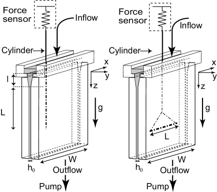
Figure 1: Left: schematic view of the experimental setup used to measure $\lambda_{||}$, $L\in[49,200]$ mm, $l=60$ mm, $W=90$ mm, $h_{0}$ is either $0.75$ or $4.9$ mm. Right: setup for measuring $\lambda_{\bot}$, $h_{0}=4.9$ mm, $L\in[20,89]$ mm.

The experimental setups used for the determination of $\lambda_{||}$ and $\lambda_{\bot}$ are shown in Fig. 1: they consist of a slit of rectangular cross section placed vertically and made of two transparent milled polymethyl methacrylate (PMMA) plates. The cell aperture has the constant value $h_{0}=4.9$ or $0.75\,\mathrm{mm}$ except in the upper $60$ mm of the cell where it increases with height from $0.75$ mm (resp. $4.9$ mm) to $5$ mm (resp. $10$ mm) for the first (resp. second) model. This Y-shape profile was designed to ease the insertion of the cylinders into the cell.

The cylinders are hung on the hook of computer controlled scales (Sartorius CP 225) measuring drag forces of the flowing fluid on the cylinder in a range of $10^{-7}$ to $8\times 10^{-1}\,\mathrm{N}$. A precision translation stage allows one to displace the cylinders across the gap of the cell: in this way, the hydrodynamic forces can be measured as a function of the distance from the walls. Furthermore, the latter are transparent allowing one to determine precisely the location of the cylinders within the cell. For the cell with the largest aperture, side views can also be obtained so that the distance separating the cylinder from the walls may also be measured; this also allows one to control the parallelism of the object with respect to the wall.

A gear pump sucks the fluid at the bottom side of the cell and reinjects it into a bath covering the top side (the fluid flows therefore always vertically downwards). The fluids are either pure water or water-glycerol mixtures with a relative mass concentration of glycerol ranging from $50$ to $80\%$.

The value of the viscosity $\eta$ is determined by first measuring the density $\rho$ of the solutions and their temperature before each series of experiments by means of an Anton Paar $35$N densimeter. The viscosity $\eta$ is then determined from the measured density and temperature by interpolating tabulated values. The final uncertainty on the value of the viscosity is about $3\%$ and is lower for all other parameters. The relative influence of viscous and inertial effects is characterized by the Reynolds number $Re=\rho h_{0}U/\eta$ in which $U$ is the mean velocity far from the cylinder.

Table 1: Experimental parameters corresponding to the measurements of $\lambda_{||}$. $d,\,L$: diameter and length of the cylinder; $h_{0}$: cell aperture in the constant aperture region; $\beta=d/h_{0}$; $\eta$: dynamic viscosity of the solutions. The symbols characterizing the different experiments are the same as in the experimental figures. For data corresponding to symbols ($\Box$), ($\boxplus$) and ($\boxtimes$), $L$ is the difference between the lengths of two cylinders.

	$d$(mm)	$h$(mm)	$\beta$	$L$(mm)	$\eta$(mPa.s)	symbol
glass	1.5	4.9	0.31	89	40.0	$\Box$
PMMA	3.2	4.9	0.65	110	22.4	$\boxplus$
PMMA	4.05	4.9	0.83	100	21.7	$\boxtimes$
optical fiber	0.14	4.9	0.029	195	35.0	$\lhd$
polyester	0.20	4.9	0.041	177	17.5	$\Diamond$
polyester	0.20	4.9	0.041	177	7.34	$\triangledown$
silk	0.45	4.9	0.092	153	37.2	$\rhd$
glass	1.5	4.9	0.31	151	6.5	$\triangle$
glass	1.5	4.9	0.31	138	40.0	$\bigcirc$
iron	2.0	4.9	0.41	177	32.0	$\bowtie$
iron	4.0	4.9	0.82	184	37.6	$\odot$
PMMA	4.05	4.9	0.83	179	21.7	$\otimes$
polyester	0.18	0.75	0.24	135	119	$\blacktriangledown$
silk	0.45	0.75	0.6	82	24.0	$\blacktriangleright$

Measurement of $\lambda_{||}$ were performed for several cylinders with different diameters (see Tab. 1), which were either rigid (glass, copper, iron, PMMA) or flexible (polyester or silk threads). The flexible threads were stretched prior to the experiments in order to remove their residual curvature. These threads include multiple fibers so that their diameter is not constant and varies periodically. Yet, such variations were found to have a negligible effect on the drag force: in the next parts, these threads are characterized by their mean diameter.

Table 2: Values of the experimental parameters corresponding to the measurement of $\lambda_{\bot}$. All these experiments were performed on the cell of aperture $h_{0}=4.9$ mm and width $W=90$ mm; $Re<5$.

	$d$(mm)	$\beta$	range of $L$(mm)	symbol	position
steel	$0.98$	$0.20$	$85$	$\blacktriangledown$	center
glass	$1.5$	$0.31$	$37.5-88$	$\blacktriangle$	center
brass	$2.96$	$0.60$	$86.5$	$\blacksquare$	center
PMMA	$3.2$	$0.65$	$44.7-88$	$\blacklozenge$	center
PMMA	$4.05$	$0.83$	$67.5-88.7$	$\bullet$	center
glass	$1.5$	$0.31$	$37.5-84$	$\triangle$	wall
brass	$2.96$	$0.60$	$86.5$	$\square$	wall
glass	$4.15$	$0.85$	$25.4-88.8$	$\bigcirc$	wall
glass	$4.15$	$0.85$	$57.6$	$+$	wall

For measuring $\lambda_{\bot}$ (see Tab. 2), the rigid cylinders are placed horizontally in the cell of largest aperture (i.e. $h_{0}=4.9$ mm); their center is halfway between the side walls of the cell. There are hung using threads of small diameter ($100\,\mu\mathrm{m}$) as shown in the right drawing of Fig. 1. Therefore, the drag forces on the threads and on the vertical rod add up: the former is however generally small compared to the latter. Moreover, this extra force may be estimated numerically (see Sec. III) and subtracted from the measurements.

The flow rate is increased stepwise from to $Q=0$ up to $Q=400\,\mathrm{mL/min}$ (resp. $Q=1400\,\mathrm{mL/min}$) for the water glycerol mixtures (resp. for water), and then decreased down to $Q=0$. Three such cycles are performed in order to verify the reproducibility of the measurement. Figures 3 and 4 display the variations of the drag force (averaged during each constant flow rate step) as a function of the mean velocity $U$. All data points corresponding to a same value of $U$ almost coincide: this demonstrates the very good reproducibility of the measurements and the lack of hysteresis between the phases during which the flow rate is increased or decreased.

III Numerical simulation procedure

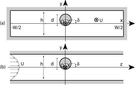
Figure 2: Schematic $2D$ representation of the experimental configuration. (a): parallel case, (b): perpendicular case

In order to determine numerically $\lambda_{||}$ and $\lambda_{\bot}$, the Stokes and incompressibility equations must be solved with appropriate boundary conditions. The shear stress and the pressure at the surface of the cylinder are then computed and added in order to determine the total hydrodynamic force. For flow parallel to the cylinders, $2D$ simulations provide reliable results; in the perpendicular configuration, $2D$ simulations have also been used but $3D$ simulations are more realistic in several cases. Figures 2 displays the geometry used in the $2D$ simulations: the pressure gradient is applied in the $z$ direction, which is along the cylinder axis for $\lambda_{||}$ (see Fig. 2a)) and perpendicular of the cylinder axis for $\lambda_{\bot}$ (see Fig. 2b).

III.1 Computation of $\lambda_{\parallel}$

For a constant pressure gradient parallel to the $z$ axis, the velocity is everywhere parallel to $z$ and $\bm{V}=V(x,y)\bm{e_{z}}$ due to the translational symmetry of the system. The governing equation of the flow then reduces to a $2D$ Laplace equation, which has been solved by means of the finite element program FreeFem++FreeFem++ . The grids contain at least $12000$ nodes (values of the force computed with a finer mesh size were identical to within $2\%$). The hydrodynamic force per unit length $f$ is computed by adding to the shear force the contribution of the pressure ($\frac{\pi}{4}\beta^{2}\partial p/\partial z$ , where $\beta=d/h_{0}$). The influence of the lateral side plates is taken into account by setting a zero-velocity boundary condition for $x=\pm W/2$. A cell of infinite width is modeled by assuming, for $x=\pm W/2$, a parabolic variation of the velocity with the distance $y$ from the midplane.

The force measured experimentally is the integral of the forces acting along the full length of the cylinder. Assuming that the velocity profile in the gap of the cell depends only on its local aperture $h(y)$ (lubrication approximation), the total force is computed numerically from:

$$F_{lub.}(L)=\int_{-l}^{L}f(z)\mathrm{d}z,$$ (1)

in which $L$ is the length of the part of the cylinder located inside the constant aperture domain (See Fig. 1) and $l$ corresponds to the part inside the Y-shaped section (in the upper fluid bath, the fluid velocity is small enough so that its contribution to the force can be neglected).

III.2 Computation of $\lambda_{\bot}$

III.2.1 $2D$ computation

Here, we consider the configuration in which the flow is normal to the cylinder (see Fig. 2b). Far from the cylinder, the velocity has a parabolic Poiseuille profile. In this $2D$ approach, the flow is assumed to be invariant in the $x$ direction so that: $\bm{V}=V_{y}(y,z)\bm{e_{y}}+V_{z}(y,z)\bm{e_{z}}$. The $2D$ Stokes equation is solved numerically by means of the Freefem++ program, using a mesh containing at least $15000$ nodes. The length of the computational domain in the $z$ direction is $8$ times its height in the $y$ direction (we checked that choosing a longer computational domain in the $z$ direction has a negligible influence on the value of the force). The shear and the pressure forces are then computed from the velocity field.

In order to validate the present method, we compared its predictions in the particular case of a cylinder located halfway between the plates to those available in the literature. In particular, Richou et al. benRichou2004 estimated analytically an asymptotical value of $\lambda_{\bot}$ in the limit when the free space between the cylinder and the walls is small ($\beta\approx 1$) by using the lubrication approximation. This approximation is valid in regions where one of the front walls and the surface of the cylinder are close to each other and nearly parallel. Since the volume flow rate is conserved along the stream-tubes, these are the same regions in which the fluid velocity is the highest (and therefore also the friction force and the pressure gradient). Rewriting these results benRichou2004 with our notations gives:

$$\lambda_{\bot}(\beta,\delta=0)\underset{\beta\rightarrow 1}{\longrightarrow}$$

$$\underbrace{6\pi\sqrt{2}\frac{{\beta}^{1/2}}{{(1-\beta)}^{3/2}}}_{\lambda_{\mathrm{shear}}}+\underbrace{9\pi\sqrt{2}\frac{{\beta}^{3/2}}{{(1-\beta)}^{5/2}}}_{\lambda_{\mathrm{pressure}}},$$ (2)

where $\delta$ is the distance between the middle of the cell and the axis of the cylinder (See Fig. 2b). The pressure term is dominant when $\beta\longrightarrow 1$. Still using the lubrication approximation, we extended this result to the case of a cylinder touching the wall in the constant aperture region (thickness of the free space equal to zero on one of the sides) with:

$$\lambda_{\bot}(\beta,\delta=(h_{0}-d)/2)\underset{\beta\rightarrow 1}{\longrightarrow}\frac{1}{2\sqrt{2}}\lambda_{\bot}(\beta,\delta=0).$$ (3)

Table 3 compares, for different values of $\beta=d/h_{0}$, the results of the present $2D$ numerical simulations to the predictions of Eq. (2) and to the theoretical and numerical results of other authors for a cylinder located halfway between the plates. The good agreement between the different values validates the present numerical procedure.

Table 3: Comparison between values of $\lambda_{\bot}$ for a cylinder halfway between the plates from the present work and from previous numerical and theoretical studies. The analytical solution of ref. benRichou2004 uses Eq. (2); all the results of the table correspond to $2D$ systems.

	Numerical	Numerical	Analytical	Analytical
$\beta$	Present work	Richou(2004)	Faxen (1946)	Richou(2004)
0.01	5.100	5.309	5.109
0.1	13.34	13.74	13.36	11.52
0.4	72.69	73.28	72.93	72.55
0.6	262.4	266.8		265.3
0.8	1850	1884		1866
0.96	$1.205\times 10^{5}$	$1.149\times 10^{5}$		$1.208\times 10^{5}$
0.99	$3.955\times 10^{6}$	$3.174\times 10^{6}$		$3.965\times 10^{6}$

III.2.2 $3D$ computation

The $2D$ approaches described above assume that the cylinder is infinitely long: they describe correctely therefore only the case of a cylinder of length equal to the width of the slit ($L=W$ in Fig. 1). If $L<W$, there is a deviation of the flow lines from the $z=cst$ planes (Fig. 2) resulting from the free space separating the edge of the cylinder and the lateral walls. If this lateral clearance is large, this reduces strongly the force on the cylinder compared to the $2D$ configuration.

In order to estimate the magnitude of this latter effect and compare the results to the experimental observations, we solved numerically the $3D$ Stokes equation in some of our experimental configurations by means of the Freefem3D program FreeFEM3D . The numerical discretization consists in a P1-P1 finite element method using penalty for the pressure stabilization; the number of vertices is at least $70000$. The ratio between the numerical lengths in the directions $x$ and $y$ is $18$ (like in the experimental cell), and the ratio between the numerical lengths in the directions $y$ and $z$ directions is $12$.

IV Experimental and numerical variations of $\lambda_{||}$

Most previous experimental studies investigated only configurations in which the cylinders are weakly confined (i.e. $\beta\ll 1$) and/or located halfway between the walls of the channel. The present experimental setup has allowed us to investigate the cases in which the confinement is strong as well as the variations of the force when the cylinder comes close to the wall.

IV.1 Variation of the drag force on a cylinder parallel to the flow with the mean velocity

In the present study, the dependence of the drag force on the geometry of the system for viscous flow is addressed. For this flow condition, the drag increases linarly with the mean flow velocity, so that $\lambda_{||}$ is independant of the velocity. Therefore, before analyzing the dependence of $\lambda_{||}$ on the geometrical parameters of the flow, we investigated the domain in which the force and the velocity are proportional for fluids of different viscosities.

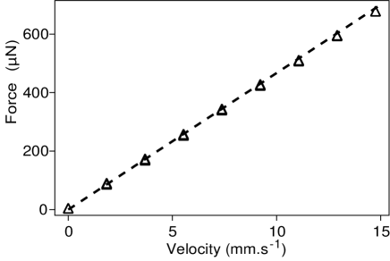
Figure 3: Variation of the force on a vertical cylinder located halfway between the plates as a function of the mean velocity $U$ of a water glycerol mixture. $d=1.5$ mm, $h_{0}=4.9$ mm, $\beta=0.3$ and $\eta=40.0$ mPa.s, Reynolds number $Re<2.2$.($\triangle$): experiments. Dashed line: numerical computation.

Figure 3 displays a set of measurements obtained using a water-glycerol mixture as the flowing fluid: the dashed line is the variation of the force with the velocity predicted by the $2D$ numerical simulations of section III.1. The difference between the experimental data and the numerical results is lower than $5\%$ for all the experiments performed in the parallel case, without any adjustable parameter. The linear increase of the force with the fluid velocity implies that the viscous effects are dominant. This is in agreement with the low value of the Reynolds number $Re$ which is less than $3$ for all the experiments using the water-glycerol solution including that of Fig. 3.

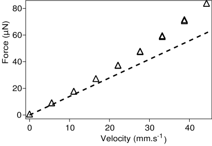
Figure 4: Same measurements as in Fig. 3 but using water ($\eta=1.0\,\mathrm{mPa.s}$): $Re\simeq 220$ for the highest flow rate. ($\triangle$): experiments. Dashed line: numerical computation.

This condition is not satisfied any more for water: in this case, the Reynolds number can be as high as $200$ and inertial effects are important even at moderate velocities as can be seen in Fig. 4. The force follows at first a linear trend with $U$: moreover, the slope at the origin is in good agreement with the theoretical value (dashed line). However, and in contrast with the case of the water-glycerol solution, the curve deviates from the linear trend at higher velocities which reflects the increase of the inertial effects: the deviation becomes large for mean velocities $U\geq 10\,\mathrm{mm.s}^{-1}$ corresponding to Reynolds numbers $Re\geq 50$. In the following, only results corresponding to the domain of linear variation of $F$ with $U$ are reported.

IV.2 Variation of $\lambda_{||}$ with the diameter

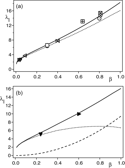
Figure 5: Variation of $\lambda_{||}$ vs. $\beta=d/h_{0}$ for cylinders located halfway between the walls. Symbols of experimental data points are defined in Tab. 1. Solid lines: $2D$ numerical predictions. (a): cell of aspect ratio $W/h_{0}\approx 18$ ($h_{0}=4.9\,\mathrm{mm}$). Dashed line: numerical value in the limit $W/h_{0}\rightarrow\infty$. (b): cells of very large aspect ratio $W/h_{0}\geq 120$ ($h=0.75\,\mathrm{mm}$); dotted line: viscous shear force term, dashed line: pressure term.

In this section, we study how confinement influences the hydraulic forces on cylinders with their axis vertical (i.e. parallel to the flow) and located halfway between the two parallel vertical walls of spacing $h_{0}$. For this purpose, we determine $\lambda_{||}$ from force measurements and we study its variation as a function of the ratio $\beta=d/h_{0}$ by using cylinders of different diameters $d$.

However, in this configuration, the local distance between the front walls varies continuously in the Y-shaped section at the top of the cell. As a result, the drag force per unit length increases continuously along the rod and is only constant in the region of constant aperture $h_{0}$. In order to determine the value of the drag specifically in this latter region, we repeat the experiment twice with cylinders of two different lengths $L_{1}$ and $L_{2}$ (large enough to reach the constant aperture domain), but otherwise identical. From Eq. (1), the difference between the forces measured at a same mean flow velocity $U$ on the two cylinders is: $\Delta F=\lambda_{||}\,\eta\,U\,(L_{1}-L_{2})$.

Figure 5a displays (solid lines) the variation of $\lambda_{||}$ with $\beta$ predicted from the $2D$ numerical simulations, for a cell of aspect ratio $W/h_{0}=18$ (i.e. of aperture $h_{0}=4.9\,\mathrm{mm}$). Values obtained by subtracting the forces measured for two cylinders of different lengths (($\Box,\boxplus,\boxtimes$) symbols) are in good agreement with the numerical model.

In the present experiments, the part $l$ of the length of the cylinder inside the Y-shaped section is generally much smaller than the length $L$ inside the constant aperture zone. In this case, we estimate $\lambda_{||}$ from a single measurement of the force $F$ by assuming that, although the local aperture $h(z)$ varies, $\lambda_{||}$ is the same in all sections and that the corresponding local mean velocity is $U(z)=h_{0}\,U/h(z)$ (in order to insure mass conservation). Eq.(1) becomes then: $F=\lambda_{||}\eta U(L+\int_{-l}^{0}(h/h(z))\mathrm{d}z)$ with $h(z)=h_{0}+(h_{0}-h_{i})z/l$ ($h_{i}$ is the aperture at the top of the Y-shaped section). $\lambda_{||}$ is then related to the force $F$ by: $\lambda_{||}=F/(\eta\,U\,L^{*})$ in which $L^{*}=L+l\,h_{0}\,ln(\frac{h_{i}}{h_{0}})/(h_{i}-h_{0})$ is an equivalent length. All data points, except those corresponding to the ($\Box,\boxplus,\boxtimes$) symbols in Figure 5a, were obtained by this “equivalent length” method: its validity is demonstrated by the small difference between values obtained for same experimental parameters by the two methods ($\otimes$ and $\boxtimes$ symbols).

Points ($\Diamond$) and ($\triangledown$) correspond to the same experimental configuration except for the viscosity which differs by a factor of $2$: they coincide within experimental error which confirms that the force is proportional to the viscosity.

In figure 5a, experimental data points are (as expected) closer to the numerical values taking into account the finite aspect ratio $W/h_{0}=18$ of the cell (solid line) than to those assuming an infinite width $W$ (dashed line). The difference between the two curves is however only of the order of $10\%$, indicating that the effect of the lateral boundaries is weak. This correction becomes completely negligible for the narrower cell ($h_{0}=0.75$ mm and $W/h_{0}=120$) and the results are then the same as for $W/h_{0}\rightarrow\infty$. In this case, it is more difficult to control experimentally the position of the cylinders: the two experimental values obtained (using the equivalent length approach) are, however, in good agreement with the numerical predictions (see Figure 5b).

Still in the high aspect ratio limit, we computed numerically the pressure force term (dashed line in Fig. 5b) and the shear force term (dotted line in Fig. 5b). On the one hand, for $\beta>0.2$, the viscous contribution levels off and decreases for $\beta>0.8$; on the other hand, the pressure contribution increases sharply when $\beta$ increases. For $\beta>0.2$, the sum of the two contributions (i.e. $\lambda_{||}$) increases almost linearly with $\beta$ ($\lambda_{||}\approx 2.1+13.8\,\beta$), and does not diverge for $\beta=1$, due to the weak perturbation of the flow.

IV.3 Variation of $\lambda_{||}$ with the location of the cylinder in the aperture

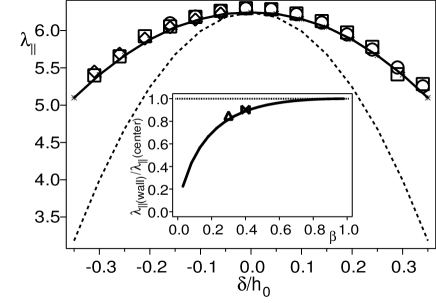
Figure 6: Variation of $\lambda_{||}$ with the normalized distance $\delta/h_{0}$ from the middle plane ($|\delta/h|<|0.5-d/(2h_{0})|=0.35$) for $d=1.5$ mm and $h_{0}=4.9$ mm. Other parameters are the same as for the ($\triangle$) symbols in Tab. 1. ($\Box$, $\Diamond$, $\circ$): repeat experimental runs for the same parameter values as ($\triangle$). Solid line: numerical computation of the force; dashed line: Poiseuille profile. Insert: variation of the ratio of the values of $\lambda_{||}$ at the wall and at the center as a function of $\beta$. ($\triangle$) and ($\bowtie$): experimental values; solid line: numerical computations.

The experimental setup also allows one to move precisely the cylinder across the gap of the cell. The normalized distance $\delta/h_{0}$ along $y$ of the axis of the cylinder from the middle plane of the cell is then determined with a precision better than $50\,\mu\mathrm{m}$ using the side view pictures. The experimental values of $\lambda_{||}$ are plotted as a function of $\delta/h_{0}$ in Fig. 6 : in this case, the sequence of displacements towards and away from the walls is performed three times. For all the values of $\beta$ considered in the present work, this curve has a parabolic shape with a maximum for $\delta/h_{0}=0$. The coefficient $\lambda_{||}$ decreases when approaching the wall (solid line Fig. 6) but less than if it followed a parabolic variation for a Poiseuille velocity profile with no cylinder present (dashed line). The influence of the finite diameter of the cylinder, particularly when it is of the order of the distance to the wall, accounts for this difference.

The insert of Figure 6 displays the variation with $\beta$ of the ratio of the values of $\lambda_{||}$ for a cylinder in contact with the walls and in the middle of the cell. This curve is well fitted by the function $1-0.9\times\exp(-3.4\beta)$ in the range $0.03\leq\beta\leq 1$. Even though the overall variation is always parabolic, the decreasing trend of $\lambda_{||}$ near the wall is stronger for lower values of $\beta$; for $\beta\ll 1$, this variation is expected to be similar to the Poiseuille parabolic profile.

V Experimental and numerical variations of $\lambda_{\bot}$

While the cylinder perturbs only weakly the flow when its axis is parallel to it, the perturbation is much larger in the perpendicular configuration. More precisely, the flow section may be significantly reduced in the vicinity of the cylinder, particularly as the normalized diameter $\beta=d/h_{0}\rightarrow 1$. This blockage effect forces the fluid to flow around the cylinder: it increases the local velocity and pressure gradient and, therefore, the drag force $F$. Paragraph V.1 reports measurements of $F$ for different values of $\beta$ and for various locations of the cylinder in the slit section (but always for $L\simeq W$). As in the parallel case (see section IV.1), only experiments in which the drag force is proportional to the velocity are used (this corresponds to a Reynolds number lower than $5$).

The blockage effect discussed above is reduced when the cylinders do not span the full width $W$ of the slit (i.e. $L<W$): then, a part of the flow takes place between the ends of the cylinder and the side walls. This bypass effect reduces in turn the drag force $F$. Paragraph V.2 reports experimental measurements of the variation of $\lambda_{\bot}$ as a function of $L/W$ together with the $3D$ numerical simulations which are needed to reproduce the highly three-dimensional bypass flows.

We observed that, when perpendicular to the flow, the cylinders move towards the middle of the cell while remaining parallel to the plates (except for short cylinders) even for Reynolds numbers as low as $0.1$. Such a repulsion effect has already been reported by Juarez2000 ; Zovatto2001 and is related to inertial effects of small magnitude (in a pure viscous flow, the lift would be zero  GHP ). In contrast, the studies of Zovatto and Juarez Juarez2000 ; Zovatto2001 predicted an attraction by the walls due to variation of the shear in the slit gap, resulting in a shift - increasing with the Reynolds number - of the equilibrium position toward the walls. However, this phenomenon was observed only for Reynolds number larger than $80$ while the present study deals with Reynolds number ($Re<5$); this effect may therefore be expected to be negligible in the present work and the cylinders should reach (as indeed observed) an equilibrium in the middle plane of the cell.

V.1 Variation of $\lambda_{\bot}$ with the diameter and the location of the cylinder in the aperture

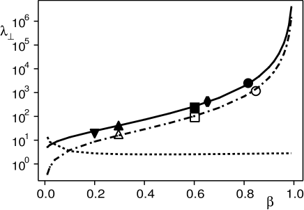
Figure 7: Variation of $\lambda_{\bot}$ as a function of $\beta$ for $L\approx W$. Cylinder in contact with a wall: open symbols (experiments); dashed dotted line ($2D$ numerical computations). Cylinder in the middle plane of the cell: filled symbols (experiments); solid line ($2D$ numerical computations, see Tab. 3). Dotted line: ratio of the values corresponding to the solid and dashed dotted lines.

In these experiments, the length of the cylinder is chosen as close as possible to the width of the cell ($0.93<L/W<1$) in order to minimize the lateral bypass flow (this point is discussed in detail in the next subsection). In this case, Figure 7 displays the variation of $\lambda_{\bot}$ as a function of $\beta$, both for cylinders located in the middle plane of the cell and in contact with the front wall; this latter case is achieved experimentally by inserting a magnetic wire in the cylinder and attracting it with a magnet.

Here, too, the experimental results and the $2D$ numerical simulations agree (to better than $10\%$). Experimental values of $\lambda_{\bot}$ up to $2500$ are measured while, as shown in Fig. 5, the maximal value of $\lambda_{||}$ is about $18$; such large values and the divergence of $\lambda_{\bot}$ when $\beta\rightarrow 1$ are due to the small gap left for the flow between the cylinder and the front walls. As this gap decreases, the pressure drop corresponding to a given constant flow rate rises strongly, leading to a sharp increase of the drag force $F$ on the rod.

When the axis of the cylinder is in the middle plane of the cell, the minimum hydraulic aperture of each of the two spaces between the cylinder and the nearest wall is $h_{0}(1-\beta)/2$ and the flows in both flow paths add up. If the rod is displaced from its equilibrium position and touches one of the walls along its full length, there is only one flow path of minimum hydraulic aperture $h_{0}(1-\beta)$ (i.e. twice the previous one). In the lubrication limit ($\beta\rightarrow 1$), the pressure drop $\Delta p$ for a given flow rate $q$ varies as the power $-5/2$ of the hydraulic aperture as shown by Eq. (2). Even taking into account the fact that the flow takes place in a single channel, this variation with the aperture is fast enough so that the drag force is lower in the configuration in which the cylinder touches the wall: more quantitatively, from Eq. (3), the coefficient $\lambda_{\bot}$ decreases by a factor $2\sqrt{2}$ from its value in the centered position. This difference between the drag forces measured in these two locations of the cylinder is indeed observed experimentally as shown in Fig. 7 (dashed line).

The case $L\approx W$ seems therefore to correspond well to the $2D$ configuration studied numerically Dvinsky1987 ; benRichou2004 ; Champmartin2007 ; however, when the cylinder is shorter than the width $W$ of the slit, flow may be perturbed (particularly when $\beta\rightarrow 1$) so that the $2D$ approximations do not reproduce well the observations. These effects will now be investigated.

V.2 Variation of $\lambda_{\bot}$ with the length of the cylinder.

In this section, the variation of the transverse drag coefficient $\lambda_{\bot}$ is studied as a function of the normalized length $L/W$ characterizing the lateral confinement.

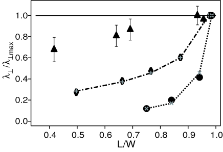
Figure 8: Variation of the normalized drag coefficient $\lambda_{\bot}/\lambda_{\bot}^{max}$ as a function of the normalized length of the cylinder $L/W$, for cylinders of different diameters located in the middle plane of the cell. ($\blacktriangle$), ($\blacklozenge$) and ($\bullet$) symbols correspond respectively to experiments for $\beta=0.31$, $0.65$ and $0.83$ (see Tab. 2 for more details). Dashed-dotted and dashed line: $3D$ numerical results obtained for $\beta=0.65$ and $0.83$.

The experimental variations of $\lambda_{\bot}$ with $W$ for three cylinders of different diameters $d$ have first been compared. For each cylinder, the maximum value $\lambda_{\bot}^{max}$ of $\lambda_{\bot}$ is reached when $L/W$ is close to $1$. In this case, the values of $\lambda_{\bot}^{max}$ are close to the predictions of $2D$ simulations (see Fig.7); small fluctuations are observed and are likely due to experimental uncertainties (inhomogeneities of the cell aperture and cell roughness for instance).

Figure 8 displays the experimental variation (symbols) of the normalized ratio $\lambda_{\bot}/\lambda_{\bot}^{max}$ with $L/W$ in the range $0.42\leq L/W\leq 0.99$. As $L/W$ decreases away from $1$, the ratio $\lambda_{\bot}/\lambda_{\bot}^{max}$ becomes significantly lower than $1$; this variation occurs earlier and is particularly strong when $\beta$ is large: for instance, for $\beta=0.83$, $\lambda_{\bot}/\lambda_{\bot}^{max}$ decreases by $60\,\%$ for a small reduction of $L/W$ by $5\,\%$. This sharp variation is due to the partial diversion of the flow into the free space between the ends of the rod and the side walls which, in turn, reduces the drag force $F$. As observed in Fig. 8, this bypassing effect is particularly strong when the clearance at the end of the cylinder is large (low values of $L/W$) while the interval between the surface of the cylinder and the two parallel walls is small (when $\beta\rightarrow 1$).

In order to predict numerically the variations of $\lambda_{\bot}/\lambda_{\bot}^{max}$, the full $3D$ flow velocity field ${\bf v}(x,y,z)$ must be determined, and not only the components $v_{y}(y,z)$ and $v_{z}(y,z)$ as before. This has been achieved by using the $3D$ version of the Freefem program (see Sec.III). As a validation test, we consider first the special situation in which the length of the cylinder is equal to the width of the cell ($L=W$). If, in addition, a perfect slip condition is used for the side walls, then the $3D$ and $2D$ simulations are equivalent and similar results should be obtained. Actually, $3D$ simulations predict values of $\lambda_{\bot}$ larger than $2D$ ones by $20\,\%$ or less: this difference is likely due to computational limitations related to the minimal practical value of the mesh size.

These $3D$ simulations were then performed for different values of $L/W$ and for two different normalized diameters $\beta$ corresponding to actual experiments. The dotted and dashed-dotted lines in Fig 8 connect the data points corresponding to the ratios $\lambda_{\bot}/\lambda_{\bot}^{max}$ obtained from these simulations (the values of $\lambda_{\bot}^{max}$ are those obtained in the validation simulations for $L=W$). The experimental and numerical variations of $\lambda_{\bot}/\lambda_{\bot}^{max}$ with $L/W$ are in very good agreement. This confirms that, in this geometry, the variations of the drag force with $L/W$ reflect $3D$ modifications of the flow structure and cannot be accounted for by $2D$ models.

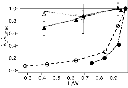
Figure 9: Variation of the normalized drag coefficient $\lambda_{\bot}/\lambda_{\bot}^{max}$ as a function of the normalized length $L/W$ for two cylinders of different diameters located either in the middle plane of the cell (filled symbols) or near a wall (open symbols). ($\triangle$,$\blacktriangle$) and ($\circ$, $\bullet$) symbols correspond respectively to $\beta=0.31$ and $0.83$ (see Tab. 2). Lines are guides for eyes.

The variation of $\lambda_{\bot}$ with the distance of the rod from the middle plane of the cell has also been investigated: as shown in Sec. V.1, the drag force should be lower when the rod is in contact with one of the front walls than when it is located halfway between them. We compared the experimental variations of $\lambda_{\bot}/\lambda_{\bot}^{max}$ with $L/W$ in both configurations: the results obtained for two values of the normalized diameter $\beta$ are displayed as symbols in Fig. 9. The drop of the coefficients when $L$ decreases is more pronounced for a cylinder halfway between the walls. This can be explained by the different relative magnitude of the hydraulic impedance of the flow paths between the ends of the rod and the side walls and of the direct paths between the rod and the front walls.

Finally, the influence of the viscosity has been investigated by comparing the results of experiments using identical parameters but fluids with two different viscosities: $\eta=50\,\mathrm{mPa.s}$ ($+$) and $\eta=30\,\mathrm{mPa.s}$ ($\circ$). The points coincide, which confirms that the drag force is proportional to the viscosity.

VI Conclusion

The experiments and numerical simulations reported in the present paper have allowed one to determine the influence of confinement effects on the drag force $F$ on a static rigid cylinder in a viscous flow inside a rectangular slit. Significantly different results have been obtained in the cases of cylinders with their length parallel and perpendicular to the mean flow, although, in both cases, $F$ is proportional to the mean velocity and the viscosity in the range investigated and can, therefore, be characterized by drag coefficients $\lambda_{||}$ and $\lambda_{\bot}$.

In the parallel case, $\lambda_{||}$ increases linearly with the confinement parameter $\beta=d/h_{0}$ but does not diverge for $\beta=1$; $\lambda_{\bot}$ increases much faster with $\beta$ and diverges near $\beta=1$ (due to the blockage of the flow) when the length $L$ of the cylinder is close to the width $W$ of the slit. $2D$ numerical simulations in planes respectively perpendicular (for $\lambda_{||}$) and parallel (for $\lambda_{\bot}$ and $L\simeq W$) to the mean flow reproduce well the results obtained in these two cases. In the perpendicular case analytical model based on the lubrication also provides a good agreement, still for $L\simeq W$ and for a strong enough confinement (i.e. for $\beta>0.2$).

When the cylinders are shorter than the width $W$ of the slit, a bypass flow appears in the space between the between the edges of the cylinder and the side walls of the slit: this reduces the direct flow in the gap between the front walls and the cylinders. This effect is particularly strong when the confinement parameter $\beta$ is close to $1$; it results in a sharp decrease of the coefficient $\lambda_{\bot}$. $3D$ numerical simulations are needed in order to predict quantitatively this effect.

The present experiments also provided evidence for an inertial lift force in the case of cylinders perpendicular to the flow direction. This force was observed for Reynolds numbers as low as $0.1$ and kept the cylinders in the middle plane of the model: this may explain recent observation of the depinning of fibers trapped inside fractures Dangelo2008 . This observation may be contrasted with numerical simulations Juarez2000 ; Zovatto2001 which predict an opposite effect, i.e. a force pushing the cylinder towards the walls. This latter force should however appear only at larger Reynolds numbers: further studies are needed to investigate these issues.

The present study dealt only with motionless rigid cylinders inside a viscous flow. Extending these studies to the measurement of forces on moving cylindrical objects, both rigid and flexible, will make the results applicable to the motion of freely swimming microorganisms Diluzio2005 .

- (1) B. Wong and S. Green, “A novel device to measure pulp fiber hydrodynamics”, Tappi Journal 2, 19–23 (2003).
- (2) N. M. K. Yasuda and K. Nakamura, “A new visualization technique for short fibers in a slit flow of fiber suspensions”, International Journal of Engineering Science 40, 1037–1052 (2002).
- (3) X. Ku and J. Lin, “Fiber orientation distribution in slit channel flows with abrupt expansion for fiber suspensions”, Journal of Hydrodynamics 20, 696–705 (2008).
- (4) A. B. Richou, A. Ambari, and J. K. Naciri, “Drag force on a cylinder midway between two parallel plates at very low reynolds numbers-part1: Poiseuille flow (numerical)”, Chem. Eng. Sci. 59, 3215–3222 (2004).
- (5) D. Czaplewski, B. Ilic, M. Zalalutdinov, W. Olbricht, A. Zehnder, H. Craighead, and T. Michalske, “A micromechanical flow sensor for microfluidic applications”, J. of Microelectromechanical Systems 13, 576–585 (2004).
- (6) K. K. Berk Yesin, K. Vollmers, and B. Nelson, “Modeling and control of untethered biomicrorobots in a fluidic environment using electromagnetic fields”, The International Journal of Robotics Research 25, 527–535 (2006).
- (7) E. Guyon, J. Hulin, L. Petit, and C. Mitescu, Physical Hydrodynamics (Oxford) (2001).
- (8) G. K. Batchelor, “Slender-body theory for particles of arbitrary cross-section in stokes flow”, J. Fluid. Mech. 44, 419–440 (1970).
- (9) R. G. Cox, “The motion of long slender bodies in a viscous fluid. part1. general theory”, J. Fluid. Mech. 44, 791–810 (1970).
- (10) N. J. de Mestre, “Low-reynolds-number fall of slender cylinders near boundaries”, J. Fluid. Mech. 58, 641–656 (1973).
- (11) Y. Takaisi, “The drag on a circular cylinder moving with low speeds in a viscous liquid between two parallel walls”, Phys. Fluids 10, 685–693 (1955).
- (12) E. Y. Harper and I.-D. Chang, “Drag on a cylinder between parallel walls in stokes’ flow”, Phys. Fluids 10, 83–88 (1967).
- (13) D. F. Katz, J. R. Blake, and S. L. Paveri-Fontana, “On the movement of slender bodies near plane boundaries at low reynolds number”, J. Fluid. Mech. 72, 529–540 (1975).
- (14) A. B. Richou, A. Ambari, M. Lebey, and J. K. Naciri, “Drag force on a cylinder midway between two parallel plates at re¡¡1 part2: moving uniformly (numerical and experimental)”, Chem. Eng. Sci. 60, 2535–2543 (2005).
- (15) J. F. Stalnaker and R. G. Hussey, “Wall effects on cylinder at low reynolds number”, Phys. Fluids 22, 603 (1979).
- (16) C. M. White, “The drag of cylinders in fluids at low speeds”, Proc. R. Soc. London Ser. A 186, 472–479 (1945).
- (17) R. Bouard and M. Coutanceau, “étude théorique et expérimentale de l’écoulement engendré par un cylindre en translation uniforme dans un fluide visqueux en régime de stokes”, Z. angew. Math. Phys. 37, 673–684 (1986).
- (18) R. Bouard, “Détermination de la trinée engendrée par un cylindre en translation pour des nombres de reynolds intermédiaires”, Z. angew. Math. Phys. 48, 584–596 (1997).
- (19) A. S. Dvinsky and A. S. Popel, “Motion of a rigid cylinder between parallel plates in stokes flow”, Computers & Fluids 15, 405–419 (1987).
- (20) S. Champmartin and A. Ambari, “Kinematics of a symetrically confined cylindrical particle in a ”stokes-type” regime”, Phys. Fluids 19, 073303 (2007).
- (21) L. Zovatto and G. Pedrizetti, “Flow about a circular cylinder between parallel walls”, J. Fluid Mech. 440, 1305–1320 (2001).
- (22) H. Juárez, R. Scott, and R. M.-B. Bagheri, “Direct simulation of freely rotating cylinders in viscous flows by high-order finite element methods”, Computers & Fluids 29, 547–582 (2000).
- (23) M. Sahin and R. G. Owens, “A numerical investigation of wall effects up to high blockage ratios on two-dimensional flow past a confined circular cylinder”, Phys. Fluids 16, 1–25 (2004).
- (24) T. Zisis and E. Mitsoulis, “Viscoplastic flow around a cylinder kept between parallel plates”, J. Non-Newtonian Fluid Mech. 105, 1–20 (2002).
- (25) R. P. Bharti, R. P. Chhabra, and V. Eswaran, “Two-dimensional steady flow of power-law fluids across a circular cylinder in a plane confined channel: Wall effects and drag coefficients”, Ind. Eng. Chem. Res. 46, 3820–3840 (2007).
- (26) M. A. Dhahir and K. Walters, “On non-newtonian flow past a cylinder in a confined flow”, J. Rheol 33, 781–804 (1989).
- (27) F. Rehimi, F. Alaoui, S. B. Nasrallah, L. Doubliez, and J. Legrand, “Experimental investigation of a confined flow downstream of a circular cylinder centred between two parallel walls”, Journal of Fluids and Structures 24, 855–882 (2008).
- (28) J. Happel and H. Brenner, Low Reynolds number hydrodynamics (Martinus Nijhoff) (1986).
- (29) C. Frei, P. Lüscher, and E. Wintermantel, “Thread-annular flow in vertical pipes”, J. Fluid. Mech. 410, 185–210 (2000).
- (30) N. A. Park and T. F. Irvine, “Falling cylinder viscosimeter end correction factor”, Rev. Sci. Instrum. 66, 3982–3984 (1995).
- (31) F. Hecht, O. Pironneau, A. le Hyaric, and K. Ohtsuka, Freefem++ manual (www.freefem.org/ff++) (2008).
- (32) S. D. Pino and O. Pironneau, FreeFEM3D manual (http://www.freefem.org/ff3d) (2008).
- (33) M. D’Angelo, H. Auradou, G. Picard, M. Poitzch, and J. Hulin, “Single fiber transport by a fluid flow in a fracture with rough walls: influence of the fluid rheology”, http://fr.arxiv.org/abs/0809.0443 (2008).
- (34) W. DiLuzio, L. Turner, M. Mayer, P. Garstecki, D. Weibel, H. Berg, and G. Whitesides, “Escherichia coli swim on the right-hand side”, Nature 435, 1271–1274 (2005).