Realization of Topological Quantum Computation with surface codes

Abstract

In this paper, the degenerate ground states of $Z_{2}$ topological order on a plane with holes (the so-called surface codes) are used as the protected code subspace to build a topological quantum computer by tuning their quantum tunneling effect. Using a designer Hamiltonian - the Kitaev toric-code model as an example, we study quantum tunneling effects of the surface codes and obtain its effective theory. Finally, we show how to do topological quantum computation including the initialization, the unitary transformation and the measurement.

I Introduction

Quantum computers are predicted to utilize quantum states to process tasks far faster than those of conventional classical computers. Various designs have been proposed to build a quantum computer, such as manipulating electrons in a quantum dot or phonon in ion traps, cavity QED, nuclear spin by NMR techniques. DiVincenzo pointed out that in order to build a real quantum computerde , the following five criterions should be satisfied : 1) Scalability of extendible qubits; 2) Initialization (Creation of highly entangled states); 3) Local operations on multi-qubit; 4) Measurement of entangled states; 5) Long decoherence time. In particular, the fifth criteria (low decoherence condition) becomes a trouble to reach the goal.

Recently, people find that it may be possible to incorporate intrinsic fault tolerance into a quantum computer - topological quantum computation (TQC) which has the debilitating effects of decoherence and free from errors. The key point is to store and manipulate quantum information in a “non-local” way, namely, the “non-local” properties of a quantum system remain unchanged under local operations. An interesting idea to realize fault-tolerant quantum computation is anyon-braiding, proposed by Kitaevk1 ; k2 . He pointed out that the degenerate ground states of a topological order make up a protected code subspace (the topological qubit) free from errorwen ; ioffe .

Topological order is a new type of quantum orders beyond Landau’s symmetry breaking paradigmwen1 ; wen2 ; wen3 . People know that there are two types of topological orders in two dimensional $S=1/2$ spin models - non-Abelian topological ordered state and $Z_{2}$ topological ordered state. Those topological ordered states may appear in frustrated spin systems or dimer modelsspin1 ; spin2 ; spin3 . Because of full gapped excitations, these topological orders are robust against any perturbations, even those perturbations that break all symmetries.

In non-Abelian topological orders, the elementary excitation are non-Abelian anyon with nontrivial statistics. Now people focus on realizing TQC by braiding non-Abelian anyonsk2 ; sa1 . The degenerate states undergoes a nontrivial unitary transformation when a non-Abelian anyon moves around the other. One can initial, manipulate and measure the degenerate ground states with several non-Abelian anyonsk2 ; sa1 , which has become a hot issue recently pa ; sarma ; du1 ; zoller ; vid ; vids ; zhang ; zhang1 ; gao ; kou1 .

On the contrary, $Z_{2}$ topological order is the simplest topological ordered state with three types of quasi-particles: $Z_{2}$ charge, $Z_{2}$ vortex, and fermionswen4 . $Z_{2}$ charge and $Z_{2}$ vortex are all bosons with mutual $\pi$ statistics between them. The fermions can be regarded as bound states of a $Z_{2}$ charge and a $Z_{2}$ vortex. In the last decade, several exactly solvable spin models with $Z_{2}$ topological orders were found, such as the Kitaev toric-code model k1 , the Wen’s plaquette model wen4 ; wen5 and the Kitaev model on a honeycomb lattice k2 . In Ref.kou1 , an alternative way to design TQC is proposed by manipulating the toric codes - the protected code subspace of $Z_{2}$ topological orders. To manipulate the degenerate ground states we can tune tunneling by controlling external field on spin models. However, to build a real quantum computer, multi-qubit is necessary. It is indeed a challenge to realize a spin model on a manifold with higher genus in experiments. To solve this problem, in this paper we design TQC by manipulating the surface code (See detail in the main content) rather than toric code, since it is more easy to make a hole in a surface.

The paper is organized as follows. In Sec. II, we study the properties of the surface code. In Sec. III, an effective theory of the surface code in $Z_{2}$ topological orders is formalized. By using the Kitaev toric-code model as an example, we demonstrate how to control the surface code by tuning the tunneling of the degenerate ground stateswen ; wen1 ; wen2 ; wen3 . In Sec. IV, based on the effective theory, the TQC is shown including the initialization, the unitary transformation and the measurement. Finally, we draw the conclusions in Sec. V.

II Degenerate ground states as surface codes

In the paper, we demonstrate the TQC in $Z_{2}$ topological order by using a designed model - the Kitaev toric-code model (an effective model of the Kitaev model on two dimensional hexagonal lattice) as an examplek1 ; k2 ; wen . Here the Hamiltonian of the Kitaev toric-code model is described by k1

$$H=-g(\sum\limits_{i\in\mathrm{even}}{Z_{i}}+\sum\limits_{i\in\mathrm{odd}}{X_{i})}.$$ (1)

where

$${Z_{i}=}\sigma_{i}^{z}\sigma_{i+\hat{e}_{x}}^{z}\sigma_{i+\hat{e}_{x}+\hat{e}_{y}}^{z}\sigma_{i+\hat{e}_{y}}^{z},\text{ }{X_{i}=}\sigma_{i}^{x}\sigma_{i+\hat{e}_{x}}^{x}\sigma_{i+\hat{e}_{x}+\hat{e}_{y}}^{x}\sigma_{i+\hat{e}_{y}}^{x}$$

with $g>0.$ $\sigma_{i}^{x,y,z}$ are Pauli matrices on sites $i.$ See the scheme in Fig.1.

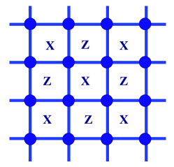
Figure 1: The scheme of the Kitaev toric-code model

Firstly we study the ground state degeneracy $\mathcal{Q}$ of the Kitaev toric-code model. The ground state is a $Z_{2}$ topological state that is denoted by ${Z_{i}=X_{i}\equiv+1}$ at each site with energy,

$$E_{0}=-g\mathcal{N}$$ (2)

where $\mathcal{N}$ is the total lattice numberwen ; wen4 ; wen5 ; kou2 . Under the periodic boundary condition (on a torus), the degeneracy $\mathcal{Q}$ is dependent on $\mathcal{N}$ : $\mathcal{Q}=4$ on even-by-even ($e\ast e$) lattice, $\mathcal{Q}=2$ on other cases (even-by-odd ($e\ast o$), odd-by-even ($o\ast e$) and odd-by-odd ($o\ast o$) lattices)wen ; wen4 ; wen5 ; kou2 . In addition, on a manifold with high genus ($\chi>1$), $\mathcal{Q}$ becomes $4^{\chi}$ on $e\ast e$ lattice and $4^{\chi}-2$ on other cases. Kitaev have noted the degenerate ground states of the Kitaev toric-code model on a torus as the toric code. On the other hand, for the ground states of the Kitaev toric-code model on a surface with open boundary condition, the ground state degeneracy now becomes

$$\mathcal{Q}=2^{n}$$ (3)

(without considering the edge states)hole ; edge . Here $n$ is the number of holes. In the following part we call the degenerate ground states of the Kitaev toric-code model on a surface with open boundary condition the surface codes.

To classify the degeneracy of the ground states (the surface codes), we define three types of closed string operators $W_{c}(\mathcal{C}),$ $W_{v}(\mathcal{C})$ and $W_{f}(\mathcal{C})=W_{c}(\mathcal{C})W_{v}(\mathcal{C}).$ Here $W_{c}(\mathcal{C})=\prod_{\mathcal{C}}\sigma_{i}^{x}$ (or $W_{v}(\mathcal{C})=\prod_{\mathcal{C}}\sigma_{i}^{z}$) is the products of spin operators along a loop $C$ connecting even-plaquettes (or odd-plaquettes) of neighboring links, with $\mathcal{C}$ denoting closed loops. It is obvious that the three types of closed string operators ($W_{c}(\mathcal{C}),$ $W_{v}(\mathcal{C})$, $W_{f}(\mathcal{C})$) correspond to three quasi-particles ($Z_{2}$ charge, $Z_{2}$ vortex, and fermions) respectively. One can easily check the commutation relations between the closed string operators and the Hamiltonian

$$\left[H,\text{ }W_{c}(\mathcal{C})\right]=\left[H,\text{ }W_{v}(\mathcal{C})\right]=\left[H,\text{ }W_{f}(\mathcal{C})\right]=0.$$ (4)

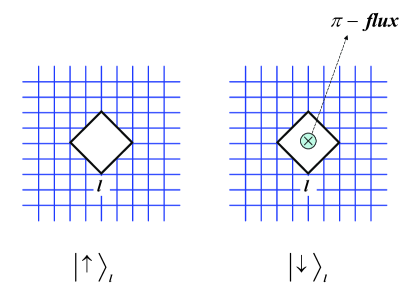
Figure 2: Mapping the qubit of a hole onto a pseudo-spin

In particular, for the surface codes, we can define two types of special closed string operators, $W_{v}(\mathcal{C}_{A})$ and $W_{f}(\mathcal{C}_{B}).$ Here $\mathcal{C}_{A}$ denotes a closed loop around a hole (labeled by an index $l$) and $\mathcal{C}_{B}$ denotes a loop from the hole to the boundary of the system. Although $W_{f}(\mathcal{C}_{B})$ is not the original closed string operator, its topological properties are the same. Due to the anti-commutation relation between $W_{v}(\mathcal{C}_{A})$ and $W_{f}(\mathcal{C}_{B})$,

$$\left\{W_{v}(\mathcal{C}_{A}),W_{f}(\mathcal{C}_{B})\right\}=0,$$ (5)

we may identify $W_{v}(\mathcal{C}_{A})$ and $W_{f}(\mathcal{C}_{B})$ as pseudo-spin ($S=\frac{1}{2}$) operators $\tau_{l}^{z}$ and $\tau_{l}^{x}$, respectively. The ground states become the eigenstates of $\tau_{l}^{z}$. Then one has two degenerate ground states (denoted by $\mid m_{l}\rangle$) for the case with a single hole. For $m_{l}=0,$ we have

$$\tau_{l}^{z}\mid m_{l}\rangle=\mid m_{l}\rangle,$$ (6)

and for $m_{l}=1$ we have

$$\tau_{l}^{z}\mid m_{l}\rangle=-\mid m_{l}\rangle.$$ (7)

Physically, the topological degeneracy arises from presence or the absence of $\pi$ flux of $Z_{2}$ vortex through the hole (See Fig.2). The values of $m_{l}$ reflect the presence ($m_{l}=1$) or the absence ($m_{l}=0$) of the $\pi$ flux in the hole.

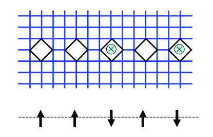
Figure 3: Mapping the qubits of a line of holes onto a pseudo-spin chain

Furthermore for the $Z_{2}$ topological order with $n$ holes, the degenerate ground states have $2^{n}$ fold degeneracy as Eq.(3). The $2^{n}$ degenerate ground states can be mapped onto a $2^{n}$-level quantum system of pseudo-spins $\mathbf{\hat{\tau}}_{l}$ by the following correspondence,

$$\mid m_{l}=0\rangle\rightarrow\mid\uparrow\rangle_{l},\text{ }\mid m_{l}=1\rangle\rightarrow\mid\downarrow\rangle_{l}.$$

We now get $2^{n}$ degenerate ground states of a chain of $n$ holes. The $2^{n}$ degenerate ground states are denoted by

$$\mid m_{1},...,m_{l}...,m_{n}\rangle=\mid m_{1}\rangle\otimes...\otimes\mid m_{l}\rangle...\otimes\mid m_{n}\rangle,$$

where the two degenerate ground states of each hole are denoted by $\mid m_{l}\rangle,$ $m_{l}=0,$ $1$. In the following parts we use the degenerate ground states on a surface with a chain of holes to do TQC (See Fig.3).

III Perturbative approach of quasi-particles

In this section we study the properties of the quasi-particles. In this solvable model, $Z_{2}$ vortex is defined as ${Z_{i}=-1}$ at even sub-plaquette and $Z_{2}$ charge is ${X_{i}=-1}$ at odd sub-plaquette. The mass gap of $Z_{2}$ charge and $Z_{2}$ vortex is $2g$. In particular, the bound states of a $Z_{2}$ charge and a $Z_{2}$ vortex on two neighbor plaquettes obey fermionic statistic. All quasi-particles in this model have flat bands. The energy spectra are $E_{v}=E_{c}=2g$ for $Z_{2}$ vortex and $Z_{2}$ charge, $E_{f}=4g$ for fermions, respectively. In other words, the quasi-particles cannot move at all.

Under the perturbation

$$\hat{H}^{\prime}=\sum\limits_{i}\mathbf{h}\cdot\mathbf{\sigma}_{i}=h^{x}\sum\limits_{i}\sigma_{i}^{x}+h^{y}\sum\limits_{i}\sigma_{i}^{y}+h^{z}\sum\limits_{i}\sigma_{i}^{z},$$ (8)

the quasi-particles begin to hop. The term $h^{x}\sum\limits_{i}\sigma_{i}^{x}$ drives the $Z_{2}$ vortex without affecting fermion and $Z_{2}$ charge. For a $Z_{2}$ vortex at $i$ plaquette ${X_{i}=-1,}$ when $\sigma_{i}^{x}$ acts on $i+\hat{e}_{x}$ site, it hops to $i+\hat{e}_{x}-\hat{e}_{y}$ plaquette denoted by ${X_{i+\hat{e}_{x}-\hat{e}_{y}}=-1},$

$${X_{i}}{=+1\rightarrow X_{i}=-1,}\text{ }{X_{i+\hat{e}_{x}-\hat{e}_{y}}}{=+1\rightarrow X_{i+\hat{e}_{x}-\hat{e}_{y}}=-1.}$$

Moreover, a pair of $Z_{2}$ vortices at $i$ and $i+\hat{e}_{x}-\hat{e}_{y}$ plaquettes can be created by the operation of $\sigma_{i}^{x},$

$${X_{i}}{=+1\rightarrow X_{i}=-1,}\text{ }{X_{i+\hat{e}_{x}-\hat{e}_{y}}}{=+1\rightarrow X_{i+\hat{e}_{x}-\hat{e}_{y}}=-1}\text{.}$$

Similarly, the term $h^{z}\sum\limits_{i}\sigma_{i}^{z}$ drives the $Z_{2}$ charge without affecting fermion and $Z_{2}$ vortex. In particular, there exist two types of fermions : the fermions on the vertical links and the fermions on the parallel links. The term $h^{y}\sum\limits_{i}\sigma_{i}^{y}$ drives fermions hopping without affecting $Z_{2}$ vortex and $Z_{2}$ charge : the fermions on the vertical links move vertically and the fermions on the parallel links move parallelly. That means both types of fermions cannot turn round any more.

To describe the dynamics of the quasi-particles we use the perturbative approach in Ref.zoller ; vid ; vids ; vid1 ; vid2 ; kou1 . In the perturbative approach, the spin operators are represented by hopping terms of quasi-particles,

$$\sigma_{i}^{x} \rightarrow (\phi_{1,i}^{{\dagger}}\phi_{1,i+e_{x}\pm e_{y}}+\phi_{1,i}^{{\dagger}}\phi_{1,i+e_{x}\pm e_{y}}^{{\dagger}}+h.c.),$$ (9)

$$\sigma_{i}^{z} \rightarrow (\phi_{2,i}^{{\dagger}}\phi_{2,i+e_{x}\pm e_{y}}+\phi_{2,i}^{{\dagger}}\phi_{2,i+e_{x}\pm e_{y}}^{{\dagger}}+h.c.),$$

$$\sigma_{i}^{y} \rightarrow (\phi_{3,i_{3}}^{{\dagger}}\phi_{3,i_{3}\pm e_{x}}+\phi_{3,i_{3}}^{{\dagger}}\phi_{3,i_{3}\pm e_{x}}^{{\dagger}}+h.c.)$$

$$+(\phi_{4,i_{4}}^{{\dagger}}\phi_{4,i_{4}\pm e_{y}}+\phi_{4,i_{4}}^{{\dagger}}\phi_{4,i_{4}\pm e_{y}}^{{\dagger}}+h.c.).$$

Here $\phi_{\alpha,i_{\alpha}}^{{\dagger}}$ ( $\alpha=1,2$ ) are the generation operator of $Z_{2}$ vortex, $Z_{2}$ charge and $\phi_{\alpha,i_{\alpha}}^{\dagger}$ ( $\alpha=3,4$ ) are the generation operator of fermions, respectively. $i_{1}$ denotes the position on even sub-plaquette and $i_{2}$ denotes the position on odd sub-plaquette. $i_{3}$ denotes the position on the vertical links and $i_{4}$ denotes the position on the parallel links. In addition, one should add a single occupation constraint (hard-core constraint) as

$$(\phi_{\alpha,i}^{{\dagger}})^{2}|\Psi\rangle=|\Psi\rangle\text{ or }\phi_{\alpha,i}^{{\dagger}}|\Psi\rangle=\phi_{\alpha,i}|\Psi\rangle$$ (10)

where $|\Psi\rangle$ denotes quantum state of the Kitaev toric-code model. Therefore, by the perturbation method, the Hamiltonian $\hat{H}=\hat{H}_{0}+\hat{H}^{\prime}$ can be represented by generation (or annihilation) operators of quasi-particles,

$$\hat{H}_{0} \rightarrow 2g\sum\limits_{i_{1}}\phi_{1,i_{1}}^{{\dagger}}\phi_{1,i_{1}}+2g\sum\limits_{i_{2}}\phi_{2,i_{2}}^{{\dagger}}\phi_{2,i_{2}}$$ (11)

$$+4g\sum\limits_{i_{3}}\phi_{3,i_{3}}^{{\dagger}}\phi_{3,i_{3}}+4g\sum\limits_{i_{4}}\phi_{4,i_{4}}^{{\dagger}}\phi_{4,i_{4}}$$

and

$$\hat{H}^{\prime} \rightarrow -h^{x}\sum\limits_{\langle i_{1},j_{1}\rangle}(\phi_{1,i_{1}}^{{\dagger}}\phi_{1,j_{1}}+\phi_{1,i_{1}}^{{\dagger}}\phi_{1,j_{1}}^{\dagger})$$

$$-h^{z}\sum\limits_{\langle i_{1},j_{1}\rangle}(\phi_{2,i_{2}}^{{\dagger}}\phi_{2,j_{2}}+\phi_{2,i_{2}}^{{\dagger}}\phi_{2,j_{2}}^{\dagger})$$

$$-h^{y}\sum_{i_{3}}(\phi_{3,i_{3}}^{{\dagger}}\phi_{3,i_{3}\pm e_{x}}+\phi_{3,i_{3}}^{{\dagger}}\phi_{3,i_{3}\pm e_{x}}^{{\dagger}})$$

$$-h^{y}\sum_{i_{4}}(\phi_{4,i_{4}}^{{\dagger}}\phi_{4,i_{4}\pm e_{y}}+\phi_{4,i_{4}}^{{\dagger}}\phi_{4,i_{4}\pm e_{y}}^{{\dagger}})$$

$$-h^{x}h^{z}\sum_{\left\langle i_{3},j_{4}\right\rangle}(\phi_{3,i_{3}}^{{\dagger}}\phi_{4,j_{4}}+\phi_{3,i_{3}}^{{\dagger}}\phi_{4,j_{4}}^{{\dagger}})+h.c..$$

In the following parts, we consider only the perturbation as $\hat{H}^{\prime}=h^{x}\sum\limits_{i}\sigma_{i}^{x}+h^{y}\sum\limits_{i}\sigma_{i}^{y}.$ The perturbative Hamiltonian of the quasi-particles becomes $\hat{H}_{v}+\hat{H}_{c}+\hat{H}_{f}$ where

$$\hat{H}_{v} = 2g\sum\limits_{i_{1}}\phi_{1,i_{1}}^{{\dagger}}\phi_{1,i_{1}}-h^{x}\sum\limits_{\langle i_{1},j_{1}\rangle}(\phi_{1,i_{1}}^{{\dagger}}\phi_{1,j_{1}}+\phi_{1,i_{1}}^{{\dagger}}\phi_{1,j_{1}}^{\dagger})+h.c.$$

$$\hat{H}_{c} = 2g\sum\limits_{i_{2}}\phi_{2,i_{2}}^{{\dagger}}\phi_{2,i_{2}}$$

$$\hat{H}_{f} = 4g\sum\limits_{i_{3}}\phi_{3,i_{3}}^{{\dagger}}\phi_{3,i_{3}}+4g\sum\limits_{i_{4}}\phi_{4,i_{4}}^{{\dagger}}\phi_{4,i_{4}}-h^{y}\sum_{i_{3}}(\phi_{3,i_{3}}^{{\dagger}}\phi_{3,i_{3}\pm e_{x}}+\phi_{3,i_{3}}^{{\dagger}}\phi_{3,i_{3}\pm e_{x}}^{{\dagger}})$$ (13)

$$-h^{y}\sum_{i_{4}}(\phi_{4,i_{4}}^{{\dagger}}\phi_{4,i_{4}\pm e_{y}}+\phi_{4,i_{4}}^{{\dagger}}\phi_{4,i_{4}\pm e_{y}}^{{\dagger}})+h.c..$$

That means $Z_{2}$ charge cannot move any more.

For the perturbative Hamiltonian on $L_{y}\times L_{x}$ square lattice ($L_{y},$ $L_{x}$ are all even integers), we obtain the dispersion of quasi-particles. The energy of $Z_{2}$ vortex is given by

$$\varepsilon_{k_{1}}=\sqrt{(\xi_{k_{1}}+2g)^{2}-\xi_{k_{1}}^{2}}$$ (14)

where

$$\xi_{k_{1}}=2h^{x}[\cos(k_{x}+k_{y})+\cos(k_{x}-k_{y})].$$ (15)

Here $k_{x}$ and $k_{y}$ are the wave vectors (The lattice constant has been set to be unit). The energy gaps of $Z_{2}$ vortex is obtained as $2g\sqrt{1-\frac{4h^{x}}{g}}.$ On the other hand, the energies of fermion is given by

$$\varepsilon_{k_{3}} = \sqrt{(\xi_{k_{1}}+4g)^{2}+4(h^{y}\cos k_{x})^{2}}$$ (16)

$$\varepsilon_{k_{3}} = \sqrt{(\xi_{k_{4}}+4g)^{2}+4(h^{y}\cos k_{y})^{2}}$$

The energy gaps of fermion is obtained as $4g\sqrt{1-\frac{2h^{y}}{g}}$. Thus one may manipulate the dispersion of $Z_{2}$ vortex and fermion by tuning the external field.

IV Effective pseudo-spin model of surface codes

It is known that the degenerate ground states of $Z_{2}$ topological orders have identically energy in thermodynamic limit. However, in a finite system,  the degeneracy of the ground states is (partially) removed due to tunneling processes, of which a virtual quasi-particle moves around the holes before annihilated with the otherk1 ; wen ; ioffe . In general cases, one will get very large energy gaps $m_{\alpha}$ ($\alpha=1,2,3,4$) for all quasi-particles and very tiny energy splitting of the degenerate ground states $\Delta E$. That is $\Delta E\ll m_{\alpha}$. Based on this condition ($\Delta E\ll m_{\alpha}$), we may ignore excited states with $E>m_{\alpha}$ and consider only the topological degenerate ground states. Thus we get a $2^{n}$ system as the effective pseudo-spin model of the surface code. In the followings, we will derive this model step by step.

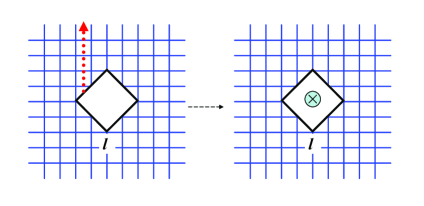
Figure 4: Tunneling process of Fermions from one hole to the boundary

In face, the closed string operators $W_{v}(\mathcal{C}_{A})$ and $W_{f}(\mathcal{C}_{B})$ can be considered as quantum tunneling processes of virtual quasi-particle moving along the loops. Let us take the quantum tunneling process of fermions as an example : at first a pair of the fermions is created. One fermion propagates around the hole driven by the operator $\sigma_{i}^{y}$ and then annihilates with the other. Then a closed string of $\sigma_{i}^{y}$ is left on the tunneling path behind the virtual fermion, that is just a closed string operator $W_{f}(\mathcal{C}_{B})$. Such a process effectively adds the $\pi$ flux to one hole and changes $m_{l}$ by $1$.

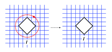
Figure 5: Tunneling process of $Z_{2}$ vortex moving around one hole

Firstly we calculate the the effective pseudo-spin model of single qubit (labeled by $l$-th hole) from tunneling processes. When a virtual fermion propagates from the boundary of the $l$-th hole to the boundary of the system, the quantum state $\left(\begin{array}[]{c}\mid\uparrow\rangle_{l}\\ \mid\downarrow\rangle_{l}\end{array}\right)$ turns into

$$\left(\begin{array}[]{c}\mid\downarrow\rangle_{l}\\ \mid\uparrow\rangle_{l}\end{array}\right)=\tau_{l}^{x}\left(\begin{array}[]{c}\mid\uparrow\rangle_{l}\\ \mid\downarrow\rangle_{l}\end{array}\right).$$ (17)

Such process is shown in Fig.4. By a degenerate perturbation approachk1 ; wen ; ioffe ; yu , one may obtain the energy splitting $\Delta E$ of the two ground states as

$$\delta E=\sum\limits_{j}\text{ }\langle\uparrow\mid_{l}\hat{H}^{\prime}(\frac{1}{E_{0}-\hat{H}_{0}}\hat{H}^{\prime})^{j}\mid\downarrow\rangle_{l}$$ (18)

which becomes

$$\delta E=2\frac{(h^{y})^{\tilde{L}^{y}}}{(-8g)^{\tilde{L}^{y}-1}}$$ (19)

where $\tilde{L}^{y}$ is the length of the shortest path of a fermion from the boundary of the $l$-th hole to the boundary of the system. See detailed calculation in Ref.yu .

On the other hand, considering a virtual $Z_{2}$ vortex propagating around the hole (shown in Fig.5), the quantum states $\left(\begin{array}[]{c}\mid\uparrow\rangle_{l}\\ \mid\downarrow\rangle_{l}\end{array}\right)$ turn into

$$\left(\begin{array}[]{c}\mid\uparrow\rangle_{l}\\ -\mid\downarrow\rangle_{l}\end{array}\right)=\tau_{l}^{z}\left(\begin{array}[]{c}\mid\uparrow\rangle_{l}\\ \mid\downarrow\rangle_{l}\end{array}\right).$$ (20)

The corresponding energy difference $\varepsilon$ of the two ground states is

$$\varepsilon=2\frac{(h^{x})^{\tilde{L}^{x}}}{(-4g)^{\tilde{L}^{x}-1}}$$ (21)

where $\tilde{L}^{x}$ is the length of the shortest path of a $Z_{2}$ vortex around the hole.

Thus the dynamics of such a two-level quantum system (a single qubit) can be described by a simple effective pseudo-spin Hamiltonian

$$\mathcal{H}_{\mathrm{eff}} = \frac{\delta E}{2}(\mid\uparrow\rangle_{l}\langle\downarrow\mid_{l}+\mid\downarrow\rangle_{l}\langle\uparrow\mid_{l})+\frac{\varepsilon}{2}(\mid\uparrow\rangle_{l}\langle\uparrow\mid_{l}-\mid\downarrow\rangle_{l}\langle\downarrow\mid_{l})$$ (22)

$$= \tilde{h}_{l}^{x}\tau_{l}^{x}+\tilde{h}_{l}^{z}\tau_{l}^{z}$$

with $\tilde{h}_{l}^{x}=\frac{\delta E}{2}$ and $\tilde{h}_{l}^{z}=\frac{\varepsilon}{2}$.

Secondly we calculate the effective exchange interaction between two qubits. For simplicity, we consider only the perturbation as $\hat{H}^{\prime}=h^{x}\sum\limits_{i}\sigma_{i}^{x}+h^{y}\sum\limits_{i}\sigma_{i}^{y}.$ Then from Eq.(13), there exist two different tunneling processes : virtual fermion propagating from the boundary of $l$-th hole to the boundary of $(l+1)$-th hole, virtual $Z_{2}$ vortex propagating around the two holes, respectively. See Fig.6 and Fig.7. Let us calculate the ground state energy splitting from degenerate perturbation approach.

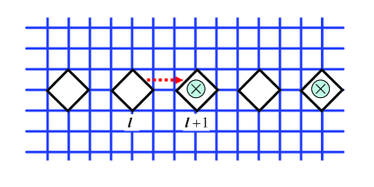
Figure 6: Tunneling process of fermions from one hole to another

When a virtual fermion propagating from the boundary of $l$-th hole to the boundary of $(l+1)$-th hole, the quantum states turn into

$$\left(\begin{array}[]{c}\mid\uparrow\rangle_{l}\\ \mid\downarrow\rangle_{l}\end{array}\right)\otimes\left(\begin{array}[]{c}\mid\uparrow\rangle_{l+1}\\ \mid\downarrow\rangle_{l+1}\end{array}\right)\rightarrow\left(\begin{array}[]{c}\mid\downarrow\rangle_{l}\\ \mid\uparrow\rangle_{l}\end{array}\right)\otimes\left(\begin{array}[]{c}\mid\downarrow\rangle_{l+1}\\ \mid\uparrow\rangle_{l+1}\end{array}\right)=\tau_{l}^{x}\mathbf{\otimes}\tau_{l+1}^{x}\left(\begin{array}[]{c}\mid\uparrow\rangle_{l}\\ \mid\downarrow\rangle_{l}\end{array}\right)\otimes\left(\begin{array}[]{c}\mid\uparrow\rangle_{l+1}\\ \mid\downarrow\rangle_{l+1}\end{array}\right).$$

Therefore, by the mapping, the pseudo-spin operator of the tunneling process of fermion corresponds to $\tau_{l}^{x}\mathbf{\otimes}\tau_{l+1}^{x}$. See Fig.6. The energy splitting $\delta E$ of the ground states is obtained as

$$\delta E=J_{l,l+1}^{xx}=\frac{(h^{y})^{L_{yy}}}{(-8g)^{L_{yy}-1}}$$ (23)

where $L_{yy}$ is the length of the shortest path from the boundary of $l$-th hole to the boundary of $(l+1)$-th hole.

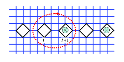
Figure 7: Tunneling process of $Z_{2}$ vortex moving around two holes

Similarly, when a virtual $Z_{2}$-vortex propagates around $l$-th and $(l+1)$-th holes, the quantum state turns into

$$\left(\begin{array}[]{c}\mid\uparrow\rangle_{l}\\ \mid\downarrow\rangle_{l}\end{array}\right)\otimes\left(\begin{array}[]{c}\mid\uparrow\rangle_{l+1}\\ \mid\downarrow\rangle_{l+1}\end{array}\right)\rightarrow\left(\begin{array}[]{c}\mid\uparrow\rangle_{l}\\ -\mid\downarrow\rangle_{l}\end{array}\right)\otimes\left(\begin{array}[]{c}\mid\uparrow\rangle_{l+1}\\ -\mid\downarrow\rangle_{l+1}\end{array}\right).$$

The pseudo-spin operators of the tunneling process of $Z_{2}$ vortex correspond to $\tau_{l}^{z}\mathbf{\otimes}\tau_{l+1}^{z}$. The tunneling amplitude is

$$J_{l,l+1}^{zz}=\frac{(h^{x})^{L_{xx}}}{(-4g)^{L_{xx}-1}}$$ (24)

where $L_{xx}$ is the length of the shortest path round both $l$-th and $(l+1)$-th holes. Thus under the perturbation $\hat{H}^{\prime}=h^{x}\sum\limits_{i}\sigma_{i}^{x}+h^{y}\sum\limits_{i}\sigma_{i}^{y},$ the total effective Hamiltonian of the exchange interaction becomes

$$\mathcal{H}_{\mathrm{eff}}\simeq\sum\limits_{l}(J_{l,l+1}^{xx}\tau_{l}^{x}\tau_{l+1}^{x}+J_{l,l+1}^{zz}\tau_{l}^{z}\tau_{l+1}^{z}).$$ (25)

Finally, for a chain of ${n}$-hole, the degenerate ground states can be mapped onto a model of a ${n}$-pseudo-spin chain. By ignoring the next nearest neighbor coupling terms, the effective model of the Kitaev Toric-code model under the perturbation $\hat{H}^{\prime}=h^{x}\sum\limits_{i}\sigma_{i}^{x}+h^{y}\sum\limits_{i}\sigma_{i}^{y}$ is naturally an anisotropy Heisenberg model

$$\mathcal{H}_{\mathrm{eff}}\simeq\sum\limits_{l}(J_{l,l+1}^{xx}\tau_{l}^{x}\tau_{l+1}^{x}+J_{l,l+1}^{zz}\tau_{l}^{z}\tau_{l+1}^{z})+\sum\limits_{l}(\tilde{h}_{l}^{x}\tau_{l}^{x}+\tilde{h}_{l}^{z}\tau_{l}^{z}).$$ (26)

The effective Hamiltonian in Eq.(26) indicates that the Kitaev Toric-code model is an example of so-called topological order with controllable dispersion of quasi-particles. For example, if one adds the external field along $y$-direction only encircling two holes, $\hat{H}^{\prime}=h^{y}\sum\limits_{i}\sigma_{i}^{y}$, the effective model is reduced into

$$\mathcal{H}_{\mathrm{eff}}\simeq J_{1,2}^{xx}\tau_{1}^{x}\tau_{2}^{x}+\tilde{h}_{1}^{x}\tau_{1}^{x}+\tilde{h}_{2}^{x}\tau_{2}^{x}.$$ (27)

So one may adjust each parameters in the effective Hamiltonian by controlling the local distribution of the external field along special direction.

V Topological quantum computation with surface codes

To design a topological quantum computer, one needs to do arbitrary unitary operations on the surface codes. Then by adding the specific perturbations to the Kitaev Toric-code model, $H^{\prime},$ one can change different quasi-particles’ hopping and then manipulate the surface codes by controlling tunneling splitting of degenerate ground states. In this part we show the initialization, the unitary transformation and the measurement.

V.1 Initialization

Firstly we will show how to initialize the system into the quantum state $\mid\uparrow,...,\uparrow\rangle$. The basic idea is to polarize all pseudo-spins by adding an effective field along x-direction and then removal it slowly. This process will occur according to the Hamiltonian

$$H^{\prime}{=h}^{x}{(t)\sum\limits_{i}}\mathbf{\sigma}_{i}^{x}$$ (28)

where ${h}^{x}{(t)=h}_{0}{e}^{-t_{0}/t}$. At the beginning, there is a finite external field ${h}^{x}{(t)\rightarrow h}_{0}$, $t\rightarrow-\infty.$ At the time $t=0,$ the external field disappears, ${h^{x}(t)=0}$. From Eq.26, we get the effective pseudo-spin Hamiltonian of the surface codes

$$\mathcal{H}_{\mathrm{eff}}\simeq\sum\limits_{l}J_{l,l+1}^{zz}\tau_{l}^{z}\tau_{l+1}^{z}+\sum\limits_{l}\tilde{h}_{l}^{z}(t)\tau_{l}^{z}$$ (29)

where $J_{l,l+1}^{zz}=\frac{[h^{x}(t)]^{L_{xx}}}{(-4g)^{L_{xx}-1}}$ and $\tilde{h}_{l}^{z}(t)=\frac{[h^{x}(t)]^{\tilde{L}^{x}}}{(-4g)^{\tilde{L}^{x}-1}}.$ Here ${h}_{0}$ is positive and $\tilde{L}^{x}$ is an even number. Then if the system evolves adiabatically and continuously from high temperature to the ground state, after a long time, the final state can be a pure state of the topological order $\mid\uparrow,...,\uparrow\rangle$ which becomes the initial state prepared for TQC.

V.2 Unitary operations

Secondly we discuss how to do an arbitrary unitary transformation on the surface codedu1 ; zhang ; zoller . The key point here is that the unitary operations can be achieved by controlling the external field along particular direction within fixed times.

A general pseudo-spin rotation operator of $l$-th qubit is defined by

$$U_{l}(\theta,\text{ }\varphi,\text{ }\gamma)=e^{-\frac{i}{\hbar}\gamma\tau_{l}^{z}}e^{-\frac{i}{\hbar}\varphi\tau_{l}^{x}}e^{-\frac{i}{\hbar}\theta\tau_{l}^{z}}$$ (30)

where $\gamma=\tilde{h}_{l}^{z}\Delta{t}_{\gamma},$ $\theta=\tilde{h}_{l}^{z}\Delta{t}_{\theta}$ and $\varphi=\tilde{h}_{l}^{x}\Delta{t}_{\varphi}.$ One can use external field along different directions encircling only $l$-th hole to do TQC : firstly applying the external field along y-direction at an interval $\Delta{t}_{\theta}{.}$ The effective Hamiltonian becomes $\mathcal{H}_{\mathrm{eff}}=\tilde{h}_{l}^{z}\tau_{l}^{z}$. Then, we swerve the external field along x-direction at an interval $\Delta{t}_{\varphi}{.}$ The effective Hamiltonian becomes $\mathcal{H}_{\mathrm{eff}}=\tilde{h}_{l}^{x}\tau_{l}^{x}$. Finally, the external field along y-direction is added at an interval $\Delta{t}_{\gamma}{.}$ The effective Hamiltonian becomes $\mathcal{H}_{\mathrm{eff}}=\tilde{h}_{l}^{z}\tau_{l}^{z}$.

Using such method, one can reach certain quantum operations demanded by TQC and have the ability to carry out gate operations onto the ’local’ qubit ($l$-th hole) at will,

$$\mid\Psi\rangle_{l}=\alpha\mid\uparrow\rangle_{l}+\beta e^{i\phi}\mid\downarrow\rangle_{l}$$ (31)

with $\alpha,$ $\beta\geq 0$ ($\alpha^{2}+\beta^{2}=1$). An example is the $\frac{\pi}{8}$ gate of a local qubit ($l$-th hole), of which we have the general pseudo-spin rotation operator as

$$U_{l}(\gamma{=\frac{\pi}{8},}\text{ }\theta{=0,}\text{ }\varphi=\frac{\pi}{8}).$$

One can firstly applying a global external field along y-direction at an interval $\Delta{t}_{\varphi}=\frac{\pi}{8\tilde{h}_{l}^{x}}{.}$ Then, we swerve the global external field along x-direction at an interval $\Delta{t}_{\gamma}=\frac{\pi}{8\tilde{h}_{l}^{z}}{.}$ Similarly, one may design the global Hadamard gate as a special pseudo-spin rotation operator on each qubit,

$$U_{l}(\gamma{=\frac{\pi}{4},}\text{ }\theta{=\frac{7\pi}{4},}\text{ }\varphi=\frac{\pi}{4}).$$

Thus, in principle, people are capable of to do arbitrary unitary transformation on the protected subspace by controlling the external field on given regions (for example, a close loop around one or more hole).

V.3 Measurement

Thirdly we discuss the measurement of an arbitrary quantum states of the surface codes. The central point is to measure the expected values of pseudo-spin operators by observing the quasi-particles’ interferences from Aharonov–Bohm (AB) effect.

To determine $\alpha,$ $\beta$ and $\phi$ of quantum state of the $l$-hole, $\mid\Psi\rangle_{l}=\alpha\mid\uparrow\rangle_{l}+\beta e^{i\phi}\mid\downarrow\rangle_{l},$ we need to observe both fermion interference and $Z_{2}$ vortex interference. Fig.8 is a scheme to show the AB interference.

Firstly we detect the value of $\left\langle\tau_{l}^{z}\right\rangle=\langle\Psi\mid_{l}\tau_{l}^{z}\mid\Psi\rangle_{l}$ to determine $\alpha$ and $\beta$ by AB effect from $Z_{2}$ vortex-interference. To observe the AB interference, we add a small external field, $h^{x}\rightarrow 0$ and $h^{y}=0$. Now $Z_{2}$ vortex begin to hop. There exist symmetrical paths from both sides of the hole. For example, $\gamma_{1}$ and $\gamma_{2}$ shown in Fig.8 are two symmetrical paths. Then the symmetrical trajectories will contribute to the transition amplitude $T_{i,j}$ according to :

$$T_{i,j}={\left|\psi_{i,j}^{\gamma_{1}}\right|^{2}}+{\left|\psi_{i,j}^{\gamma_{2}}\right|^{2}}+2\epsilon\left|\psi_{i,j}^{\gamma_{2}}\psi_{i,j}^{\gamma_{1}}\right|$$ (32)

where $\psi_{i,j}^{\gamma_{2}}$ and $\psi_{i,j}^{\gamma_{1}}$ are the wave functions of $Z_{2}$ vortex of the two trajectories. For the ground state $\mid\uparrow\rangle_{l}$, $\epsilon$ is unit. However, for the ground state with $\pi$-flux inside the hole $\mid\downarrow\rangle_{l},$ we have $\epsilon=-1.$ Then we can distinguish these two cases. For two symmetrical paths $\psi_{i,j}^{\gamma_{2}}=\psi_{i,j}^{\gamma_{1}}{=t}_{f}$, we get a probability $\alpha^{2}$ for $\mid\uparrow\rangle_{l}$ with $T_{i,j}=4{t_{f}^{2}}$ and a probability $\beta^{2}$ for $\mid\downarrow\rangle_{l}$ with $T_{i,j}=0$.

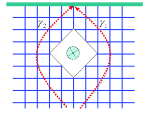
Figure 8: The scheme of the interference around $l$-th hole.

On the other hand, one can detect the value of $\left\langle\tau_{l}^{x}\right\rangle=\langle\Psi\mid_{l}\tau_{l}^{x}\mid\Psi\rangle_{l}$ to determine the parameter $\phi$ by observing fermion interference. To observe the AB interference of fermion, we add a small external field, $h^{y}\rightarrow 0$. The wave function of fermion has a periodic boundary condition from the hole to the boundary of the system for the ground state $\mid\uparrow^{\prime}\rangle_{l}=\frac{1}{\sqrt{2}}\mid\uparrow\rangle_{l}+\mid\downarrow\rangle_{l}$ and an anti-periodic boundary condition for the ground state $\mid\downarrow^{\prime}\rangle_{l}=\frac{1}{\sqrt{2}}\mid\uparrow\rangle_{l}-\mid\downarrow\rangle_{l}.$ Then an arbitrary state $\alpha\mid\uparrow\rangle_{l}+\beta e^{i\phi}\mid\downarrow\rangle_{l}$ is re-written into

$$\sqrt{\frac{1}{2}+\alpha\beta\cos\phi}e^{i\phi^{\prime}}\mid\uparrow^{\prime}\rangle_{l}+\sqrt{\frac{1}{2}-\alpha\beta\cos\phi}\beta e^{i\phi^{\prime\prime}}\mid\downarrow^{\prime}\rangle_{l}$$ (33)

where

$$\phi^{\prime}=\arctan(\frac{\sin\phi}{\beta\cos\phi+\alpha})$$ (34)

and

$$\phi^{\prime\prime}=\arctan(\frac{\sin\phi}{\beta\cos\phi-\alpha}).$$ (35)

For two symmetrical paths (one from the hole, the other not), we get a probability $(\frac{1}{2}+\alpha\beta\cos\phi)$ for $\mid\uparrow^{\prime}\rangle_{l}$ with $T_{i,j}=4{t_{v}^{2}}$ and a probability $\frac{1}{2}-\alpha\beta\cos\phi$ for $\mid\downarrow^{\prime}\rangle_{l}$ with $T_{i,j}=0$. As a result, we determine the parameters $\alpha,$ $\beta$ and $\phi$ of an arbitrary state $\mid\mathrm{vac}\rangle=\alpha\mid\uparrow\rangle_{l}+\beta e^{i\phi}\mid\downarrow\rangle_{l}$.

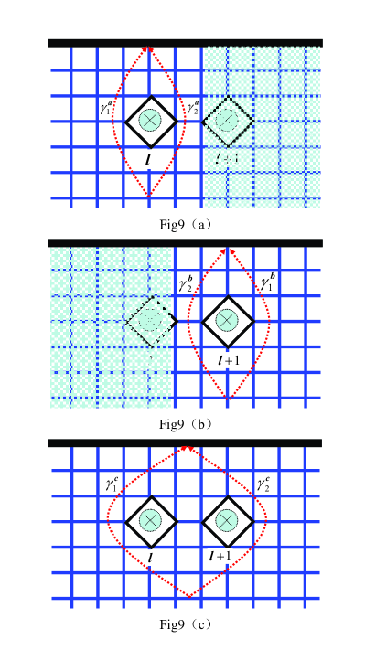
Figure 9: The scheme of the interference around $l$-th hole in (a), the interference around $l+1$-th hole in (b), and the interference around two holes in (c). Z2 vortex cannot move in shadow region.

The situation becomes more complex for $2$-qubit. For $2$-qubit with $2$ holes ($l$-th and $l+1$-th), a general entangled quantum state is given by

$$\alpha_{1} \mid \uparrow\rangle_{l+1}\otimes\mid\uparrow\rangle_{l}+\alpha_{2}e^{i\phi_{2}}\mid\uparrow\rangle_{l+1}\otimes\mid\uparrow\rangle_{l}$$

$$+\alpha_{3}e^{i\phi_{3}} \mid \uparrow\rangle_{l+1}\otimes\mid\downarrow\rangle_{l}+\alpha_{4}e^{i\phi_{4}}\mid\downarrow\rangle_{l+1}\otimes\mid\uparrow\rangle_{l}$$

Here $\alpha_{i}$ and $\phi_{i}$ are all real number. Because of the constraint, $\sum_{i}\alpha_{i}^{2}=1,$ there are totally $2(2^{2}-1)=6$ independent parameters. One can detect the value of $\left\langle\tau_{l}^{z}\right\rangle,$ $\left\langle\tau_{l+1}^{z}\right\rangle,$ $\left\langle\tau_{l}^{z}\tau_{l+1}^{z}\right\rangle$ to determine $\alpha_{i}$ $(i=1,2,3,4)$ from the AB effect of $Z_{2}$-vortex-interference by $2^{2}-1=3$ times measurements. As shown in Fig.9, there are $3$ cases of the $Z_{2}$ vortex-interference of different paths : $\gamma_{1}^{a}$ and $\gamma_{2}^{a}$ are two symmetrical paths around the hole $l$; $\gamma_{1}^{b}$ and $\gamma_{2}^{b}$ are two symmetrical paths around the hole $l-1$; $\gamma_{1}^{c}$ and $\gamma_{2}^{c}$ are two symmetrical paths around both hole $l$ and hole $l-1.$ To do the observations, we only add a small external field in the regions without shadow, $h^{x}\rightarrow 0$ and $h^{y}=0$ (In the shadow regions, there is no external field, $h^{x}=h^{y}=0$). So the $Z_{2}$-vortex is guided moving around given holes. Similarly, one can detect the value of $\left\langle\tau_{l}^{x}\right\rangle,$ $\left\langle\tau_{l+1}^{x}\right\rangle,$ $\left\langle\tau_{l}^{x}\tau_{l+1}^{x}\right\rangle$ determine $\phi_{i}$ $(i=2,3,4)$ from the AB effect of fermion-interference by $3$ times measurements.

For $n$-qubit with $n$ holes, a general entangled quantum state is given by

$$\sum_{i}\alpha_{i}e^{i\phi_{i}}\mid\uparrow\rangle_{i}\otimes\mid\uparrow\rangle_{l}\otimes\mid\uparrow\rangle_{l+1}$$ (36)

Here $\alpha_{i}$ and $\phi_{i}$ are all real number. Because of the constraint, $\sum_{i}\alpha_{i}^{2}=1,$ there are totally real $2(2^{n}-1)$ independent parameters by changing the paths of quasi-particles. So people needs to do $2(2^{n}-1)$ times measurement to determine the entangle state by changing different paths of AB interferences. One can determine $\alpha_{i}$ from $\frac{n(n+1)}{2}$ times measurements of $Z_{2}$ vortex-interference (to detect $\left\langle\tau_{l}^{z}\right\rangle,$ $\left\langle\tau_{l}^{z}\tau_{l+1}^{z}\right\rangle,$ $\left\langle\tau_{l}^{z}\tau_{l+1}^{z}\tau_{l+2}^{z}\right\rangle,$…, $\left\langle\prod_{l}\tau_{l}^{z}\right\rangle$ ) and $\phi_{i}$ from $\frac{n(n+1)}{2}$ times measurements of fermion-interference (to detect $\left\langle\tau_{l}^{x}\right\rangle,$ $\left\langle\tau_{l}^{x}\tau_{l+1}^{x}\right\rangle$), respectively. So one cannot determine all the parameters by the quasi-particles interferences if $n>3$. It is still an unsolved problem to measure a general entangled quantum state of $n$-qubit with $n$ ( $n>3$) holes.

V.4 Errors

Finally we discuss the errors and the constraint on our proposal.

Errors mainly come from the thermal effect. At finite temperature, $Z_{2}$ vortices are excited, their moving around the holes leads to errors, as causes ”thermal hopping” from one degenerate ground state to another. The decoherence time $t_{\mathrm{de}}$ has been roughly estimated by the time to stretch a pair of $Z_{2}$ vortices over a distance equal to the average inter-particle separation (This is because the energy gap of $Z_{2}$ vortex is smaller than that that of fermion). At low temperature, one can estimate that $t_{\mathrm{de}}$ is about $t_{0}e^{\frac{4g}{k_{B}T}}$ where $t_{0}=\frac{L_{p}}{v^{\ast}}$ is the time scale for $Z_{2}$ vortex moving the length of tunneling pathes, $L_{p}$ ort . $v^{\ast}$ is the average speed of $Z_{2}$ vortex, which is estimated by $v^{\ast}\sim\sqrt{\frac{k_{B}T}{M_{\mathrm{eff}}}}$ where $M_{\mathrm{eff}}\simeq\left(2h^{x}\right)^{-1}$ is the effective mass of $Z_{2}$ vortex.

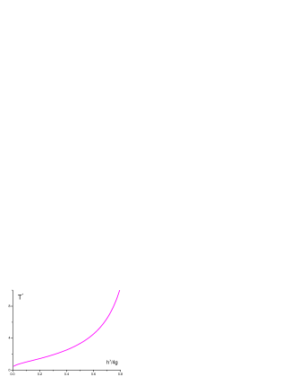
Figure 10: The crossover temperature for an example of tunneling process of Z2 vortex. The scale of temperature is $\frac{k_{B}L_{p}}{4g}$

So there must exist a crossover temperature $T^{\ast}$ from thermal hopping to quantum tunneling. Above $T^{\ast}$, the decay rate of the quantum states is determined by process of thermal activation, which is governed by the Arrhenius law,

$$t_{0}^{-1}e^{-\frac{4g}{k_{B}T}}.$$ (37)

Therefore at high temperature the errors proliferate and one cannot get reliable TQC. Below $T^{\ast}$, quantum tunneling processes dominate, the rate of which goes as $e^{-B}$ where $B$ is about

$$B\sim\max(L_{p}\ln\frac{4g}{\left|h_{x}\right|},\text{ }L_{p}\ln\frac{8g}{\left|h_{y}\right|}).$$ (38)

Ignoring the prefactor and equating the exponents, one obtains

$$T^{\ast}=\frac{4g}{k_{B}B}.$$ (39)

Fig.10 shows the crossover temperature via $h_{x}$ for a quantum tunneling process of $Z_{2}$ vortex. Thus if the temperature is kept far below $T^{\ast}$, $T\ll T^{\ast}$, one may do unitary operations safely.

However, because of the errors from the stochastic fields, we still get in trouble on storing quantum information by the surface codes. To store quantum information, all quantum tunneling processes need to be suppressed as low as possible, $e^{-B}\rightarrow 0$. That means the external fields should be removed, $h^{x}\equiv h^{y}\equiv 0$. Now the estimation of the crossover temperature in Eq.39 is invalid. Without external fields, due to the diverge effective masses of $Z_{2}$ vortex, $M_{\mathrm{eff}}\rightarrow\infty,$ one may store the quantum information for arbitrary long time, $t_{\mathrm{de}}\rightarrow\infty$. Whereas, the stochastic noise fields leads to a finite decoherence time $t_{\mathrm{de}}$. Thus to get a long-lived quantum information, both the temperature and the stochastic noise fields should be suppressed below a threshold. See detail in Ref.sta .

VI Summary

In this paper, we find an alternative way towards designing a quantum computer that may be possible to incorporate intrinsic fault tolerance. Using the Kitaev toric-code model as an example, we obtain the effective pseudo-spin model that can be mapped onto the anisotropic Heisenberg model of a pseudo-spin chain in external field. Then one may tune the parameters of the effective pseudo-spin model by controlling tunneling processes of the surface codes by applying external field along special direction on lattices. In particular, five criterions to build a quantum computer are satisfied :

1. Scalability of extendible qubits : The qubits is the so-called surface codes (two degenerate ground states of $Z_{2}$ topological orders on a plane with a hole). So the quantum computer is just a line of holes in the $Z_{2}$ topological order.

2. Initialization (Creation of highly entangled states) : We may polarize the pseudo-spins by adding an effective field along x-direction and then removing it slowly.

3. Local operations on multi-qubit : The unitary operations can do by controlling the external field along particular direction within fixed times.

4. Measurement of entangled states : We may measure the expected values of pseudo-spin operators by observing the quasi-particles’ interferences from AB effect.

5. Low decoherence : Below the crossover temperature $T^{\ast},$ the decoherence processes will be controlled as low as possible.

Finally we discuss the realization of the Kitaev toric-code model. Because it can be regarded as an effective model of the Kitaev model on a two dimensional hexagonal lattice, one may realize the Kitaev model firstly. The realization of the Kitaev model has been proposed in an optical lattice of cold atoms in Ref.du ; zo1 and in Josephson junction array of a superconductor in Ref.you . So it is possible to design a quantum computer in these system in the future.

In general. to design a topological quantum computer via quantum tunneling effect, there are four necessary conditions : 1) $Z_{2}$ topological order as the ground states; 2) controllable dispersion of quasi-particles; 3) space with nontrivial topological structure (manifold with high genus or multi-hole); 4) low temperature and low noise. Thus considering these conditions, one may do TQC based on other models.

- (1) D. P. DiVincenzo, Mesoscopic Electron Transport, eds. Sohn, Kowenhoven, Schoen (Kluwer 1997), P.657, cond-mat/9612126.
- (2) A. Kitaev, Ann. Phys. 303, 2(2003).
- (3) A. Kitaev, Ann. Phys. 321, 2(2006).
- (4) X. G. Wen, Quantum Field Theory of Many-Body Systems, (Oxford Univ. Press, Oxford, 2004).
- (5) L. B. Ioffe, et al., Nature 415, 503 (2002).
- (6) X. G. Wen, Int. J. Mod. Phys. B 4, 239 (1990).
- (7) X. G. Wen, Advances in Physics 44, 405 (1995).
- (8) X. G. Wen, Phys. Rev. B 65, 165113 (2002).
- (9) N. Read and S. Sachdev, Phys. Rev. Lett. 66, 1773 (1991).
- (10) X. G. Wen, Phys. Rev. B 44, 2664 (1991).
- (11) R. Moessner and S. L. Sondhi, Phys. Rev. Lett. 86, 1881, (2001).
- (12) X. G. Wen, Phys. Rev. D 68, 065003 (2003).
- (13) X. G. Wen, Phys. Rev. Lett. 90 (2), 016803 (2003).
- (14) S. Das Sarma, M. Freedman, C. Nayak, S. H. Simon, A. Stern, arXiv: cond-mat/0707.1889.
- (15) J. K. Pachos, Annals of Physics 322, 1254 (2007).
- (16) C. W. Zhang, S. Tewari, and S. Das Sarma, Phys. Rev. Lett. 99, 220502 (2007). S. Tewari, et al., Phys. Rev. Lett. 98, 010506 (2007).
- (17) Y.-J. Han, R. Raussendorf, and L.-M. Duan, Phys. Rev. Lett. 98, 150404 (2007).
- (18) L. Jiang, et al., Nature Phys., doi:10.1038/nphys943 (2008) doi:10.1038/nphys943.
- (19) K.P. Schmidt, S. Dusuel, and J. Vidal, Phys. Rev. Lett. 100, 057208 (2008).
- (20) S. Dusuel, K.P. Schmidt, and J. Vidal, Phys. Rev. Lett. 100, 177204 (2008).
- (21) J. Vidal, S. Dusuel, and K.P. Schmidt, Physical Review B 79, 033109 (2009).
- (22) J. Vidal, R. Thomale, K.P. Schmidt, and S. Dusuel, arXiv:0902.3547 (2009).
- (23) Chuanwei Zhang, et al., Proc. Natl. Acad. Sci. U.S.A. 104, 18415 (2007).
- (24) Chuanwei Zhang, S. L. Rolston, and S. Das Sarma, Phys. Rev. A 74, 042316 (2006). Chuanwei Zhang, V. W. Scarola, and S. Das Sarma, Phys. Rev. A 76, 023605 (2007).
- (25) C. Y. Lu, et al., Phys. Rev. Lett. 102, 030502 (2009).
- (26) S. P. Kou, Phys. Rev. Lett. 102, 120402 (2009).
- (27) S. P. Kou, M. Levin, and X. G. Wen, Phys. Rev. B 78, 155134 (2008).
- (28) E. Dennis, A. Kitaev, A. Landahl and L. Preskill, J. Math. Phys. 43, 4452 (2002).
- (29) There are two types of edge states of the Kitaev toric-code model. For a boundary parallels x-direction or y-direction, there exist the gapless edge states described by Majorana fermionswen5 ; kou2 . For a boundary along diagonal directions ( or ), there is no stable edge state. As a result, in this paper the boundary of both the holes and the system belong to belongs to the second type (along diagonal directions).
- (30) J. Yu and S. P. Kou, arXiv:0905.1156.
- (31) Z. Nussinov and G. Ortiz, Phys. Rev. B 77, 064302 (2008).
- (32) T. M. Stace, S. D. Barrett, A. C. Doherty, arXiv: quat-ph/0904.3556.
- (33) L.-M. Duan, E. Demler, and M. D. Lukin, Phys. Rev. Lett. 91, 090402 (2003).
- (34) A. Micheli, G. K. Brennen, P. Zoller, Nature Physics, 2, 341 (2006).
- (35) J. Q. You, X.-F. Shi, and F Nori, arXiv:0809.0051v1 (2008); Zheng-Yuan Xue, Shi-Liang Zhu, J. Q. You, and Z. D. Wang, Phys. Rev. A 79, 040303(R) (2009).