Charge constrained density functional molecular dynamics for simulation of condensed phase electron transfer reactions

Abstract

We present a plane-wave basis set implementation of charge constrained density functional molecular dynamics (CDFT-MD) for simulation of electron transfer reactions in condensed phase systems. Following earlier work of Wu et al. Phys. Rev. A 72, 024502 (2005), the density functional is minimized under the constraint that the charge difference between donor and acceptor is equal to a given value. The classical ion dynamics is propagated on the Born-Oppenheimer surface of the charge constrained state. We investigate the dependence of the constrained energy and of the energy gap on the definition of the charge, and present expressions for the constraint forces. The method is applied to the Ru²⁺-Ru³⁺ electron self-exchange reaction in aqueous solution. Sampling the vertical energy gap along CDFT-MD trajectories, and correcting for finite size effects, a reorganization free energy of 1.6 eV is obtained. This is 0.1-0.2 eV lower than a previous estimate based on a continuum model for solvation. The smaller value for reorganization free energy can be explained by the fact that the Ru-O distances of the divalent and trivalent Ru-hexahydrates are predicted to be more similar in the electron transfer complex than for the separated aqua-ions.

I Introduction

Atomistic simulation of electron transfer reactions has become a major task in computational physics and chemistry. This field was pioneered in the Eighties by the works of WarshelWarshel (1982); Hwang and Warshel (1987); King and Warshel (1990), Kuharski et alKuharski et al. (1988); Bader et al. (1990) and othersKakitani and Mataga (1985); Tachiya (1989); Carter and Hynes (1989). Electron donor and acceptor and the solvent were modelled with classical potential energy functions and the diabatic free energy profiles were sampled with (biased) molecular dynamics simulation. These early simulations gave unprecedented insight into electron transfer reactions and provided a first numerical confirmation for the validity of the linear response approximation of the Fe²⁺-Fe³⁺ electron self-exchange reactionKuharski et al. (1988), thus confirming a crucial assumption in Marcus theory of electron transferMarcus (1956).

The application of modern density functional molecular dynamics to electron transfer reactions has not been successful until recentlySit et al. (2006). The reason is that common exchange-correlation functionals are of limited use for this task due to their tendency to erroneously delocalize electrons, thus prohibiting an accurate modelling of charge transfer states. This deficiency termed electron self-interaction or delocalization errorZhang and Yang (1998); Mori-Sanchez et al. (2006a) is intrinsic to GGA and hybrid density functionals unless special care is taken in their parametrization. In parallel to the development of functionals with minimal self-interaction errorMori-Sanchez et al. (2006b); Cohen et al. (2007), a number of correction schemes have been proposed to minimize the delocalization error of existing and computationally inexpensive density functionalsPerdew and Zunger (1981); Tavernelli (2007); Harrison (1987); d’Avezac et al. (2005); VandeVondele and Sprik (2005), including DFT+ULiechtenstein et al. (1995); Migliore et al. (2009); Deskins and Dupuis (2009), formulation of a penalty density functionalSit et al. (2006), and constrained DFTDederichs et al. (1984); Akai et al. (1986); Wu and Van Voorhis (2005, 2006a, 2006b, 2006c, 2007); Wu et al. (2009); Behler et al. (2005, 2007); Schmidt et al. (2008). Development of such schemes are particularly important in density functional molecular dynamics, where efficient computation of the exchange-correlation energy and forces is absolutely crucial.

In recent years several groupsWu et al. (2009); Schmidt et al. (2008); Behler et al. (2007) have greatly advanced the development of the constrained DFT approach. In this method an external potential is added to the Kohn-Sham equations preventing an excess electron or hole from wrongly delocalizing over donor and acceptor ions. The external potential is varied until a given constraint on the density, for instance a charge or spin constraint, is satisfied. The search for this external potential, usually carried out within a Lagrange multiplier scheme, introduces a second iteration loop in addition to the usual self-consistent iteration of the Kohn-Sham equations. Due to the localized (or diabatic) nature of the constrained states the delocalization error of common density functionals is reduced, though not eliminated. Hence one can expect that common density functionals describe constrained states as well as any other states where delocalizing electrons are not present.

The construction of charge localized states seems to be a somewhat artificial procedure since the external potential and charge are all but uniquely defined. For large donor-acceptor distances one can expect, however, that the details of charge definition are less relevant. Thus it is appealing to use CDFT to describe the charge localized (diabatic) states of long-range electron transfer reactions. However, as it is possible to extract approximate electronic coupling matrix elements between CDFT statesWu and Van Voorhis (2006a), one can construct approximate Hamiltonian matrices in the space of constrained states (CDFT configuration interaction)Wu and Van Voorhis (2007). The adiabatic states diagonalizing this Hamiltonian suffer less from the delocalization error than unconstrained states and can be used to describe short range phenomena such as chemical bond break reactionsWu and Van Voorhis (2007); Wu et al. (2009).

All of the above mentioned calculations (except the ones described in Refs. Behler et al. (2005, 2007)) were carried out in the gas-phase using quantum chemistry codes. In this work we present a plane-wave basis set implementation of charge constrained density functional molecular dynamics (CDFT-MD) in the Car-Parrinello molecular dynamics code (CPMD)cpm . This allows us to study the electron self-exchange of the Ru²⁺-Ru³⁺ ion pair in aqueous solution at finite temperature with the solute and solvent treated at the same density functional level of theory. To our best knowledge only one such simulation has been reported previously by Sit et al.Sit et al. (2006), who developed a penalty density functional approach to simulate the isoelectronic Fe²⁺-Fe³⁺ electron self-exchange reaction in aqueous solution. A previous attempt to use a charge restraint rather than a charge constraint to drive a charge transfer reactions with Car-Parrinello molecular dynamics was also reportedSulpizi et al. (2005). However, it turned out that at reasonably high restraining forces the charge restraint does not provide enough bias for obtaining charge localized states.

In the present work we define the constraint as the charge difference between the electron donating Ru²⁺-hexahydrate and the electron accepting Ru³⁺-hexahydrate. The charge constrained state is energy optimized at each molecular dynamics step and the dynamics of the system propagated on the constrained Born-Oppenheimer surface. We then construct Marcus-type free energy profiles by calculation of the vertical energy gap between the two charge transfer states along the molecular dynamics trajectory. The reorganization free energy obtained, about 1.6 eV after correction for finite size effects, is in fair agreement with experimental estimates and other computational studies indicating that CDFT-MD can be successfully applied to electron transfer problems in the condensed phase.

This paper is organized as follows: First we briefly review the theoretical background of CDFT. Then we address the dependency of CDFT energies on the choice of the constraining potential for gas phase and condensed phase electron transfer systems. Thereafter our molecular dynamics implementation of CDFT is validated by finite temperature simulation of the H${}_{2}^{+}$ molecule. The main objective of the present work, the charge constrained density functional MD simulation of the aqueous Ru²⁺-Ru³⁺ electron self exchange reaction is presented thereafter. The results are discussed in light of experimental results, and previous classical molecular dynamics and continuum studies. At the end of this work we give a perspective on future work planned. In the appendix we give explicit expressions for constraint forces due to the charge constraint and summarize relevant technical details of CDFT-MD calculations.

II Theory

II.1 Charge constrained density functional molecular dynamics

CDFT and its working equations have been presented previously in a number of papersWu and Van Voorhis (2005, 2006a, 2006b, 2006c, 2007); Wu et al. (2009); Behler et al. (2005, 2007); Schmidt et al. (2008). Here we follow the work of van Voorhis and co-workersWu and Van Voorhis (2005) and give a short summary of the equations pertinent to our molecular dynamics implementation.

In CDFT the usual energy functional $E[\rho]$ is minimized with respect to the electron density $\rho$ under the condition that the scleronomic constraint

$$\int w(\mathbf{r})\rho(\mathbf{r})\;d\mathbf{r}=N_{\text{c}},$$ (1)

is satisfied, where $N_{\text{c}}$ is a real number. The weight function $w(\mathbf{r})$ on the left hand side of Eq. 1 defines the constraint, for instance the charge of an atom, molecule or molecular fragment, or the charge difference between groups of atoms. $N_{\text{c}}$ defines the value of the constraint. Both quantities are input parameter that remain unchanged during the constrained minimization. Using the Lagrange multiplier technique the new energy functional to be minimized is given by

$$W[\rho,V]=E[\rho]+V(\int w(\mathbf{r})\rho(\mathbf{r})\;d\mathbf{r}-N_{\text{c}}),$$ (2)

where $V$ is an as yet undetermined Lagrange multiplier. In order to find the minimum of $W[\rho,V]$ with respect to (wrt) $\rho$ and $V$, $W$ is minimized with respect to $\rho$ for a given $V$, the gradient

$$\frac{\delta W}{\delta V}\Big{|}_{\rho}=\int w(\mathbf{r})\rho(\mathbf{r})\;d\mathbf{r}-N_{\text{c}}$$ (3)

at the minimizing density is determined to generate the next iteration step for $V$, $W$ is minimized for the new value of $V$ wrt $\rho$ and this procedure is repeated self-consistently until convergence is reached, that is when $\delta W/\delta V|_{\rho}\!=\!0$ and $\delta W/\delta\rho|_{V}\!=\!0$. Efficient Newton methods can be employed for this minimization procedure since second derivatives of $W$ wrt $V$ are available analytically via density functional perturbation theoryWu and Van Voorhis (2005) or numerically as finite differences of Eq. 3. For practical applications we define in addition to the usual wavefunction convergence criterion a second convergence parameter for the constraint.

$$\mathcal{C}\geq\left|\int w(\mathbf{r})\rho(\mathbf{r})\;d\mathbf{r}-N_{\text{c}}\right|.$$ (4)

$\mathcal{C}$ is a measure of how accurately the charge constraint Eq. 1 is fulfilled.

It is interesting to note that Eq. (2) implies the following exact relation for the energy difference between two constrained states A and B, $\Delta E_{\text{AB}}$, and the continuous set of Lagrange multipliers connecting the two states, $V(N_{\text{c}})$.

$$\Delta E_{\text{AB}}=-\int_{\text{A}}^{\text{B}}V(N_{\text{c}})\;dN_{\text{c}},$$ (5)

The Lagrange multiplier can thus be interpreted as the force along the charge coordinate $N_{\text{c}}$. The parallel to thermodynamic integration is intriguing.

CDFT-MD simulation or constrained geometry optimization can be carried out provided one takes into account the additional forces $\mathbf{F}_{\text{c}i}$ arising from the constraint term on the right hand side of Eq. 2. Adopting the Hellmann-Feynman theorem the total force on atom $i$ at position $\mathbf{R}_{i}$ is given by

$$\mathbf{F}_{\text{tot},i}=\mathbf{F}_{i}+\mathbf{F}_{\text{c}i}$$ (6)

where $\mathbf{F}_{\text{tot},i}\!=\!-\partial W/\partial\mathbf{R}_{i}$, $\mathbf{F}_{i}\!=\!-\partial E/\partial\mathbf{R}_{i}$ and

$$\mathbf{F}_{\text{c}i}=-V\int\rho(\mathbf{r})\frac{\partial w(\mathbf{r},\mathbf{R})}{\partial\mathbf{R}_{i}}\;d\mathbf{r}$$ (7)

Note that the weight function can depend on the coordinates $\mathbf{R}$ of all atoms in the system. An explicit expression for the derivative in the integrand of Eq. 7 using the weight function defined below is given in appendix B. In molecular dynamics simulation the Lagrange multiplier $V$, the total energy and forces have to be calculated at each time step. The computational bottleneck is the iterative search for $V$. To improve the efficiency we have implemented an extrapolation scheme for the Lagrange multiplier using Lagrange polynomials. For details we refer to appendix C.

II.2 Definition of the charge constraint

The charge constraint is fully defined by the weight function $w$ in the integrand of Eq. 1 and the actual value of the constraint, $N_{\text{c}}$. In principle there are an infinite number of ways of how to choose the weight function. In practice one chooses the weight so that Eq. 1 corresponds to some common charge definition. One is then left to investigate how much the results depend on the charge definition used. In previous work Mulliken, Loewdin and a Becke real space integration scheme have been testedWu and Van Voorhis (2006c). While for short donor-acceptor distances the energy of the constrained state was strongly dependent on the weight used, for medium to large distances the dependence on the weight was reasonably small. The real space density integration scheme was found to give best overall performanceWu and Van Voorhis (2006a, 2007).

Building on this previous work we use a slightly different real space density integration scheme for charges, the one according to HirshfeldHirshfeld (1977). The Hirshfeld charge $q_{i}$ of an atom $i$ at position $\mathbf{R}_{i}$ is obtained by integration of the total electron density $\rho$ multiplied with an atom centered weight function $w_{i}$,

$$q_{i} = Z_{i}-\int w_{i}(\mathbf{r},\mathbf{R})\rho(\mathbf{r})\;d\mathbf{r}$$ (8)

$$w_{i}(\mathbf{r},\mathbf{R}) = \frac{\rho_{i}(\mathbf{r}-\mathbf{R}_{i})}{\sum_{j=1}^{N}\rho_{j}(\mathbf{r}-\mathbf{R}_{j})}$$ (9)

where $Z_{i}$ is the core charge in pseudopotential calculations (or the charge of the nucleus in all-electron calculations), and $N$ is the total number of atoms. The weight function is constructed from the unperturbed promolecular densities of atoms $i$, $\rho_{i}$,

$$\rho_{i}(\mathbf{r}-\mathbf{R}_{i})=\rho_{i}(r)=\sum_{j}n_{j}|\psi_{i}^{j}(r)|^{2}$$ (10)

where $r\!=\!|\mathbf{r}-\mathbf{R}_{i}|$. The sum ranges over the radial part of the promolecular atomic orbitals $\psi_{i}^{j}(r)$ with occupation number $n_{j}$. The weight $w_{i}$ is close to unity up to a distance of about one atomic radius and goes to zero according to the decay of the promolecular atomic density. Note that the sum of the Hirshfeld charges of all atoms is equal to the total charge of the system.

A natural choice for the constraint for electron transfer reactions is the charge difference between a set D of atoms comprising the electron donor and a set A of atoms comprising the electron acceptor.

$$C-\int w(\mathbf{r})\rho(\mathbf{r})\;d\mathbf{r}=\sum_{i\in D}q_{i}-\sum_{i\in A}q_{i}=N_{\text{c}}$$ (11)

where

$$w=w_{\text{D}}-w_{\text{A}}=\frac{\sum_{i\in\text{D}}\rho_{i}(\mathbf{r}-\mathbf{R}_{i})-\sum_{i\in\text{A}}\rho_{i}(\mathbf{r}-\mathbf{R}_{i})}{\sum_{j=1}^{N}\rho_{j}(\mathbf{r}-\mathbf{R}_{j})}.$$ (12)

and $\rho_{i}$ is given by Eq. 10. The constant $C$ in Eq. 11 is equal to the difference in the core charges, $C\!=\!\sum_{i\in D}Z_{i}-\sum_{i\in A}Z_{i}$, merely causing a constant shift of $W$ (Eq. 2) by $VC$. The weight function Eq. 12 used for the simulation of the Ru²⁺-Ru³⁺ electron self-exchange reaction in aqueous solution is illustrated in Fig. 1. The donor (acceptor) atoms are comprised of Ru²⁺ (Ru³⁺) and all atoms of the first solvation shell of Ru²⁺ (Ru³⁺) . Note that the sign of the weight function changes sharply at the interface of the donor-acceptor complex. Assuming that a charge equivalent to one electron is transferred, the constraint value $N_{\text{c}}$ is set equal to 1 for the initial state and equal to -1 for the final state.

While relying on the basic charge definition Eqs. 8-9, we have investigated different functional forms for the densities $\rho_{i}$ that define the atomic weight function $w_{i}$ of Eq. 9. The results are presented in section IV.3. Technical details concerning the calculation of the weight function can be found in appendix A.

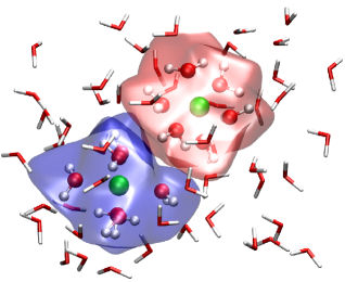
Figure 1: Isosurfaces of the weight function Eq. 12 for values $w\!=\!0.6$ (red) and $w\!=\!-0.6$ (blue). The snapshot is taken from a charge constrained MD simulation of the Ru²⁺-Ru³⁺ electron transfer complex in aqueous solution. Ru ions are depicted as green spheres and first shell water molecules are depicted in ball and stick representation. All atoms composing the Ru-hexahydrate in the upper right (lower left) part of the figure are donor (acceptor) atoms. Solvent molecules not included in the charge constraint are depicted in stick representation.

II.3 Electron transfer free energy curves

In Marcus theoryMarcus (1956) electron transfer reactions are described by two charge localized or diabatic free energy curves, one for the reactant state (A) and one for the product state (B). Electron transfer is assumed to occur at the crossing point of the two curves. In the limit of linear response the two free energy curves are parabolic and the activation free energy for electron transfer is given by

$$\Delta A^{\ddagger}=\frac{(\Delta A+\lambda)^{2}}{4\lambda}$$ (13)

where $\Delta A$ is the reaction free energy and $\lambda$ is the reorganization free energy. The latter is inversely proportional to the curvature of the free energy parabola and is a measure for the free energy required to distort the equilibrium configuration of one diabatic state to the equilibrium configuration of the other diabatic state while staying on the same free energy curve. For electron self-exchange reactions $\Delta A\!=\!0$ and the activation free energy is entirely determined by the reorganization free energy.

Following WarshelWarshel (1982) the diabatic free energy curves defining the reorganization free energy can be obtained by sampling the vertical energy gap $\Delta E$

$$\Delta E(\mathbf{R})=E_{\text{B}}(\mathbf{R})-E_{\text{A}}(\mathbf{R})$$ (14)

using molecular dynamics simulation. $E_{\text{A}}(\mathbf{R})$ and $E_{\text{B}}(\mathbf{R})$ are the charge localized (diabatic) potential energy surfaces and the vector $\mathbf{R}$ denotes the coordinates of all atoms in the system. The relative Landau free energy $A_{M}(\Delta E)$ along this coordinate is given for state $M$, $M$ = A, B, by

$$A_{M}(\Delta E)=-k_{\text{B}}T\ln p_{M}(\Delta E),$$ (15)

where $k_{\text{B}}$ is the Boltzmann constant, $T$ the temperature and $p_{M}(\Delta E)$ the probability distribution of the reaction coordinate in state $M$. If the free energy curves are parabolic the reorganization free energy is equal to the average vertical energy gap,

$$\lambda=\langle\Delta E\rangle_{\text{A}}$$ (16)

where $\langle\cdots\rangle_{\text{A}}$ denotes the usual canonical average for state A.

The free energy curves Eq. 15 can be obtained by sampling configurations with charge constrained density functional molecular dynamics in state A as described above, followed by calculation of the vertical energy gap Eq. 14 between the constrained states A ($N_{\text{c}}\!=\!1$, Eq. 11) and B ($N_{\text{c}}\!=\!-1$) for the set of sampled configurations. However, unbiased equilibrium simulations give only accurate results close to the free energy minimum of $A_{M}$ and are of limited use for regions of $\Delta E$ far away from the minimum. Fortunately, due to the exact linear free energy relation between the free energy gap and the energy gapWarshel (1982); Tachiya (1989); Tateyama et al. (2005); Blumberger et al. (2006),

$$A_{\text{B}}(\Delta E)-A_{\text{A}}(\Delta E)=\Delta E$$ (17)

it is possible to calculate a good part of the curve at high free energies accurately from equilibrium simulations. Thus, using information from two distinct regions of $\Delta E$ one can construct a reasonably accurate free energy profile without the use of computationally expensive enhanced sampling methodsBlumberger et al. (2006); Blumberger (2008).

III Computational details

Charge constrained density functional molecular dynamics has been implemented in the CPMD codecpm . Unless stated otherwise, all calculations were carried out with the BLYPBecke (1988); Lee et al. (1988) functional using a reciprocal space cutoff of $70$ Ry, Troullier-Martins pseudopotentials for nuclei+core electronsTroullier and Martins (1991), pseudoatomic densities for construction of the weight function Eq. 12, a convergence criterion for the wavefunction gradient of $1\times 10^{-5}$H and a charge constraint convergence criterion defined in Eq. (4) of $\mathcal{C}=5\times 10^{-5}$e. All calculations were carried out in the lowest spin state.

Ru²⁺-Ru³⁺ electron self-exchange was simulated in a periodic box of dimension $14.5\times 11.35\times 11.35$Å  containing two Ru ions and 63 water molecules. The donor and acceptor groups are comprised of the ion and the six water molecules forming the first solvation shell, Ru(H₂O)${}_{6}^{2+}$ and Ru(H₂O)${}_{6}^{3+}$, respectively, see Figure 1. The charge constraint Eq. 11 was set equal to 1 corresponding to the reactant diabatic state A. Pseudoatomic densities for construction of the weight function Eq. 12 were used, i.e. the charges correspond to the definition of HirshfeldHirshfeld (1977). The Ru²⁺ and Ru³⁺ aqua ions are both low spin as opposed to the corresponding aqua-ions of Fe²⁺ and Fe³⁺Sit et al. (2006). Hence, the dublet state was chosen for simulation of the aqueous ET complex. The initial configuration was taken from an equilibrated classical molecular dynamics trajectory carried out in a previous investigation of the same reactionBlumberger and Lamoureux (2008). The distance between the two Ru ions was fixed at 5.5 Å  using the RATTLE algorithm Andersen (1983). The system was simulated in the NVT ensemble at $300$ K using a chain of Nose-Hoover thermostatsMartyna et al. (1992) of length $4$ with a frequency $1000$ cm^-1. To increase the efficiency of charge constrained Born-Oppenheimer molecular dynamics we used an extrapolation scheme for prediction of the Lagrange multiplier $V$ as described in appendix C, an extrapolation scheme for the initial guess of the wavefunction, slightly higher convergence criteria of $\mathcal{C}=5\times 10^{-4}$ e for the constraint convergence and of $2\times 10^{-5}$ H for the wavefunction gradient, and an MD time step of $40\,\text{au}\!=\!0.96$ fs. With this setup the average number of iterations for $V$ were $\sim 2\!-\!3$ per molecular dynamics time step. Accordingly, the computational overhead compared to standard Born-Oppenheimer molecular dynamics without charge constraint is about a factor of 2-3. The average drift of the conserved energy was $-9.7\times 10^{-5}$H/atom/ps along a trajectory of length 6.6 ps. This is somewhat large but still acceptable for our purposes. Better energy conservation can be obtained if tighter convergence criteria and a smaller time step is used. For calculation of thermal averages the first ps of dynamics was discarded. The energy gap Eq. 14 was calculated for 225 equidistantly spaced snapshots taken from the last 5.5 ps of the trajectory using the same convergence criteria as for the MD simulation. For calculation of the product diabatic state B the constraint Eq. 11 was set equal to -1.

IV Results and discussion

Before we present the results for electron self-exchange in the condensed phase we report on a series of test calculations carried out for simple electron transfer systems in the gas phase. These include a basic validation of charge constrained single point calculations and molecular dynamics, calculation of the dissociation curve of H${}_{2}^{+}$ and He${}_{2}^{+}$ to test the correct long-range behaviour of CDFT, and an investigation of the dependence of the constrained state energies on the weight function used.

IV.1 (CO)^-

As a first test of our implementation we carried out a series of charge constrained wavefunction optimizations on the (CO)^- molecule. The distance between the C and the O atom was chosen to be $2$Å in order to avoid the problem of spin contamination which occurs for larger distances. The oxygen atom is chosen as the electron donor and the carbon atom as the electron acceptor. The excess electron is transferred from the oxygen to the carbon atom by increasing the charge difference $N_{\text{c}}$ (Eq. 11) between the atoms in small steps from -1 to 1. The Lagrange multiplier $V$ and the potential energy $E$ of the constrained states are shown in Fig. 2 as a function of $N_{\text{c}}$.

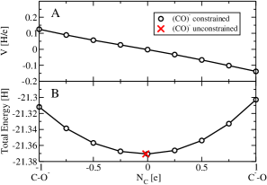
Figure 2: Lagrange multiplier $V$ (A) and potential energy $E$ (B) versus constrained charge difference $N_{\text{c}}$ between C and O atom in (CO)^-. In (B) the computed energies are indicated by circles and the running integral $-\int_{-1}^{N_{\text{c}}}V\;dN_{\text{c}}+E[\text{C}^{-}\text{O}]$ by straight lines. The potential energy and charge difference for unconstrained wavefunction optimization of (CO)^- is indicated by a cross.

According to Eq. 5 the energy difference between C^-O and CO^- should be equal to the negative of the integral of $V$ over $N_{\text{c}}$. Indeed, the difference between the end-points is $\Delta E_{\text{AB}}=E[\text{C}^{-}\text{O}]-E[\text{CO}^{-}]\!=\!9.038$ mH whereas integration gives $-\int_{-1}^{1}V\;dN_{\text{c}}\!=\!9.084$ mH. The numbers match within the given convergence criteria. Furthermore, the potential energy obtained from unconstrained calculations (denoted by a cross in Fig. 2) lies on the constrained potential energy curve at $N_{\text{c}}\approx 0$. Thus, the unconstrained state can be reproduced by constrained wavefunction optimization if a constraint value is used that is equal to the charge difference of the unconstrained state.

IV.2 Dissociation of H${}_{2}^{+}$ and He${}_{2}^{+}$

The wrong dissociation curve for H${}_{2}^{+}$ is probably one of the most spectacular failures of GGA and hybrid density functionals. The reason for this failure is well knownZhang and Yang (1998). Due to the wrong scaling behaviour of these functionals wrt electron number the charge delocalized state is predicted to be lower in energy than the charge localized state, even though the two states are degenerate in the limit of large inter-nuclear separation distance in exact theory. Using CDFT configuration interaction Wu et al. could circumvent this problemWu and Van Voorhis (2007). The authors reported a dissociation curve that matched the exact Hartree-Fock curve remarkably well at the equilibrium region and at long range.

Here we calculate the dissociation curve for H${}_{2}^{+}$ and He${}_{2}^{+}$ using a single charge constrained state in order to test the correct long range behaviour of our CDFT implementation. The constraint is again the charge difference between the two atoms. In case of He${}_{2}^{+}$ $N_{\text{c}}$ was set equal to 1 for all distances. For H${}_{2}^{+}$ the constraint value was set equal to the charge difference obtained when the promolecular pseudoatomic reference orbitals were used for construction of the initial wavefunctionWu and Van Voorhis (2007). This was necessary because a value $N_{\text{c}}\!=\!1$ would only be obtained at very high external potentials for which the wavefunction would not converge. Thus, the constraint value for H${}_{2}^{+}$ changes with distance from about $0.86$ at $2$Å to 1.0 at $4.4$Å and larger distances.

The energies of the charge constrained states of H${}_{2}^{+}$ and He${}_{2}^{+}$ relative to the (unconstrained) energy of the isolated fragments are shown in Fig. 3, together with the exact Hartree Fock curve for H${}_{2}^{+}$ and the essentially exact FCI curve for He${}_{2}^{+}$Pieniazek et al. (2007).

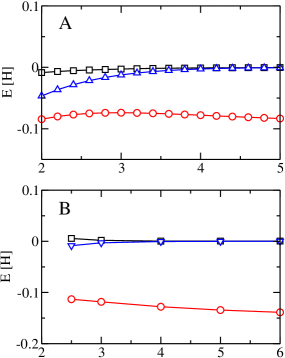
Figure 3: Dissociation curves for H${}_{2}^{+}$ (A) and He${}_{2}^{+}$ (B). Constrained and unconstrained DFT results are indicated by squares and circles, respectively. The exact Hartree-Fock curve for H${}_{2}^{+}$ and the curve for He${}_{2}^{+}$ at the FCI/aug-cc-pV5Z level of theoryPieniazek et al. (2007) are indicated by triangles, respectively.

The CDFT curves agree well with the exact curves for distances larger than  3Å. This is a considerable improvement with respect to the results of unconstrained optimizations, which give the wrong dissociation limit. It also shows that the optimization in the external potential yields the correct electronic state of the unconstrained isolated fragments. The significant deviation for smaller distances is due to the fact that only a single charge localized state is used, which can not describe chemical bonding between the fragments. The deficiency at short range can be cured using the CDFT-configuration interaction approach introduced in Ref. Wu and Van Voorhis (2007).

IV.3 Dependence on the weight function

A crucial issue in CDFT calculations is the dependence of the numerical results on the definition of the charge constraint. While relying on the basic real-space charge definition Eqs. 8-9, we have investigated different functional forms for the densities $\rho_{i}$ that define the atomic weight function $w_{i}$ of Eq. 9. Besides numerical pseudoatomic densities we have tested a minimal basis of Slater functions and a minimal basis of Gaussian functions,

$$\rho_{i}(\mathbf{r}-\mathbf{R}_{i})=\frac{N_{\text{el},i}}{\sigma_{k}\sqrt{2\pi}}e^{-\frac{(\mathbf{r}-\mathbf{R}_{i})^{2}}{2\sigma_{k}^{2}}},$$ (18)

where $\sigma_{k}$ is the width of particle species $k$ and $N_{\text{el},i}$ denotes the number of electrons of the isolated atom $i$. Using Gaussian functions one can vary the decay of the weight functions systematically simply by changing the exponent of the densities in Eq. 18. For slowly decaying densities the weight function changes sign smoothly, while for densities that match the pseudoatomic densities the sign changes sharply. In the limit of an infinitely fast decaying density $\rho_{i}$ the electron density $\rho$ at a given point in space is assigned to the atom closest to this point. This corresponds to the charge definition according to Voronoi. For the real space integration of Eq. 8 we have introduced a radial cutoff $R_{\text{c}}$ (see appendix A). Its influence on the constrained energy is also reported here.

Table 1: Charge constrained energies for hole transfer in Zn${}_{2}^{+}$. Pseudoatomic, Slater and Gaussian denote the functional form of the densities $\rho_{i}$ (Eq. 10) that define the atomic weight function $w_{i}$ of Eq. 9. $\sigma$ is the width of the Gaussian function Eq. 18 and $R_{\text{c}}$ denotes the radial weight cutoff (see appendix A).

$r=4.0$Å
weight	$\sigma$ [Å]	$R_{\text{c}}$ [Å]	Energy [H]
pseudoatomic		$3.762$	$-113.7834$
		$5.121$	$-113.7834$
Slater		$3.762$	$-113.7780$
		$5.121$	$-113.7783$
Gaussian	$0.5$	$3.762$	$-113.7859$
	$0.732$	$3.762$	$-113.7849$
	$1.0$	$3.762$	$-113.7818$
	$2.0$	$3.762$	$-113.7633$
	$1.0$	$2.56$	$-113.7813$
	$1.0$	$3.0$	$-113.7814$
	$1.0$	$5.0$	$-113.7819$

$r=2.5$Å
weight	$\sigma$ [Å]	$R_{\text{c}}$ [Å]	Energy [H]
pseudoatomic		$3.762$	$-113.7744$
		$5.121$	$-113.7745$
Slater		$3.762$	$-113.7471$
		$5.121$	$-113.7473$
Gaussian	$0.5$	$3.762$	$-113.7824$
	$0.732$	$3.762$	$-113.7755$
	$1.0$	$3.762$	$-113.7613$
	$2.0$	$3.762$	$-113.6495$
	$1.0$	$2.56$	$-113.7781$
	$1.0$	$3.0$	$-113.7612$
	$1.0$	$5.0$	$-113.7617$

The charge constrained energies of Zn${}_{2}^{+}$ obtained for different weight functions are summarized in table 1. The Zn-Zn distance was chosen to be $r=4$ Å and $r=2.5$ Å. The latter is equal to twice the covalent radius of Zn. The constraint was again the charge difference, $N_{\text{c}}\!=\!1$. Considering hole transfer at a distance $r=4$ Å, we find that the change in energy is only a few mH when the width of the Gaussian function is varied from 0.5 to 1.0 Å. If larger values for the widths are used the weight function becomes unphysically smooth and the energy increases. The energy obtained with pseudoatomic functions differ by not more than 2 mH from the energies obtained with Gaussian functions. A somewhat larger deviation is obtained for Slater functions. The cutoff $R_{\text{c}}\!=\!3.762$ Å for truncation of the weight function is sufficient for all weight functions. Overall, the dependence of the results on the weight function used is reasonably small. This is not the case for hole transfer at a smaller distance of $r=2.5$ Å. Here the details of the weight function are important. The variation in energy are a few ten mH, an order of magnitude larger than at $r=4$ Å. Hence, our results indicate that charge constrained states are well defined only if the distance between donor and acceptor is larger than at least the sum of their covalent radii.

As we are primarily interested in the aqueous Ru²⁺-Ru³⁺ electron self-exchange reaction (see section IV.5) we have investigated the dependence of the vertical energy gap Eq. 14 of this system on the functional form of the weight used. For this purpose we have taken a snapshot from the constrained MD simulation of aqueous Ru²⁺-Ru³⁺ and calculated the two charge constrained states $E_{\text{A}}$ ($N_{\text{c}}\!=\!-1$) and $E_{\text{B}}$ ($N_{\text{c}}\!=\!-1$). For the Gaussian weight function $\sigma_{\text{H}}=\sigma_{\text{O}}=0.6$Å and $\sigma_{\text{Ru}}=1.0$Å is used. See section III for further details. The results are summarized in table 2.

Table 2: Dependence of the energy gap Eq. 14 on the weight function for the aqueous Ru²⁺-Ru³⁺ electron self-exchange reaction. The charge is the sum of the atomic charges of Ru³⁺(H₂O)₆ in the final ET state.

weight	energy gap [eV]	charge [e]
pseudoatomic	$1.587$	$1.5663$
Slater	$1.732$	$1.2639$
Gaussian	$1.552$	$1.7764$

The energy gaps differ by less than $0.18$ eV for the three weights considered and are within $0.04$ eV for pseudoatomic and Gaussian weight functions. This variation is not insignificant and should be considered as a lower limit of the error of the results presented in section IV.5. More than the gap energies varies the charge of the electron donor Ru²⁺(H₂O)₆ (recall that only the charge difference between donor and acceptor is constrained). The sensitivity of the results on the weight used is probably a consequence of the close approach of the first shell water molecules that bridge the two Ru-ions. These water molecules form strong hydrogen bonds that make the constrained energy and charges susceptible to details of the weight function at the interface of the two Ru-complexes.

IV.4 CDFT-MD for H${}_{2}^{+}$

The molecular dynamics implementation of CDFT is tested by simulating an isolated H${}_{2}^{+}$ molecule on the Born-Oppenheimer surface of a single charge-constrained state. A charge difference $N_{\text{c}}\!=\!0.5$ e is enforced giving an average charge of $0.25$ e respectively $0.75$ e on the two H atoms. The system is simulated in the NVE ensemble at a temperature of approximately $300$ K using the Velocity Verlet algorithm. A value of $5\times 10^{-6}$ H for the convergence of the wavefunction gradient is used and a timestep of $20\text{au}\approx 0.48$ fs. In order to assess the dependence of energy conservation on the convergence criterion for the charge constraint, Eq. 4, we calculated a series of trajectories of length 1 ps for different values of $\mathcal{C}$. The total linear drift of the conserved energy as a function of $\mathcal{C}$ is shown in Fig. 4.

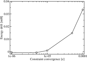
Figure 4: CDFT-MD simulation of H${}_{2}^{+}$. The linear drift in the conserved energy is shown as a function of the charge constraint convergence criterion $\mathcal{C}$ defined in Eq. 4.

The drift is less than $1\times 10^{-3}$ mH/atom/ps at $\mathcal{C}\!=\!1\times 10^{-6}$ e showing that the total energy is essentially conserved if a tight convergence criterion for the charge constraint is applied. The sharp rise of the total energy drift at a value of $\mathcal{C}\!=\!1\times 10^{-5}$ e is due to the fact that the system essentially behaves like a harmonic oscillator. Small deviations from the target constraint value can lead to a resonance between the bond vibration and the external constraint potential. This can cause instabilities in the integration of the equations of motion, which can even lead to dissociation of the molecule. Fortunately, this behaviour is rather exceptional. The resonance effect is dampened in larger systems allowing us to use less strict convergence criteria than for H${}_{2}^{+}$.

IV.5 Ru²⁺-Ru³⁺ electron self-exchange in aqueous solution

We finally present our results for the CDFT-MD simulation of Ru²⁺-Ru³⁺ electron self-exchange in the condensed, aqueous phase. The charge constraint is chosen as the charge difference between the electron donating group, Ru²⁺(H₂O)₆, and the electron accepting group, Ru³⁺(H₂O)₆, and the constraint value is $N_{\text{c}}\!=\!1$. This choice is motivated by the fact that one wants to transfer a charge corresponding to one electron from the donor to the acceptor complex. The six water molecules forming the first coordination shell are included in the constraint as the redox active orbitals are delocalized over the metal and the first coordination shell. The distance of the two Ru ions is constrained to 5.5 Å. The same distance was used in a previous classical molecular dynamics simulation of this reactionBlumberger and Lamoureux (2008). No other constraints on the dynamics are imposed. Details for the CDFT-MD simulation are summarized in section III.

During CDFT-MD the highest occupied majority spin orbital (HOMO) of the ET complex is correctly located on the donor complex, and the lowest unoccupied minority spin orbital (LUMO) is located on the acceptor complex. As expected, the two molecular orbitals are composed of a $d$ orbital of the metal $t_{2g}$ manifold and the $p$ orbitals of the ligands. Similarly to the separated aqua ions, there is no mixing with orbitals of solvent molecules beyond the first solvation shell.

As the charge difference is constrained, only, the absolute charge of donor and acceptor complex is free to vary during the dynamics run. The charge fluctuations are very small, however, $\sigma=0.05$ e. The average charge of the Ru²⁺(H₂O)₆ complex, $0.52$ e, and of the Ru³⁺(H₂O)₆ complex, 1.52 e, are significantly smaller than their formal charges of +2 e and +3 e, respectively. They are, however, similar to the charge of a single Ru²⁺(H₂O)₆ (Ru³⁺(H₂O)₆) ion in aqueous solution, 0.75 e (1.15 e). Thus, the charge constraint localizes an excess charge of $-0.23$ e (0.37 e) on the donor (acceptor) complex relative to the charge of the isolated aqua ions. The charge of the remaining solvent, 2.96 e, is more than half of the total system charge. Although some charge transfer between the ET complex and the solvent is expected, the magnitude of this effect seems rather large. The reason for this is not clear, but one may speculate that the BLYP functional tends to delocalize the total system charge, an effect that might be enhanced when periodic boundary conditions are used for simulation of the aqueous phase. Yet, the large magnitude of charge transfer to the solvent is not a particular feature of CDFT, because this effect already occurs for standard (unconstrained) GGA-DFT calculations on solutions containing a single ion.

In order to assess the effects of the charge constraint on the coordination geometry, we calculated the metal-oxygen radial distribution functions ($g_{\text{RuO}}(r)$) of Ru²⁺ and Ru³⁺ in the electron transfer complex and compare with the radial distribution function of the single aqueous ions as obtained from standard (unconstrained) Car-Parrinello molecular dynamics simulationBlumberger and Sprik (2006, 2005). The result is illustrated in Fig. 5.

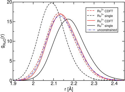
Figure 5: First peak of the radial distribution functions of Ru²⁺ and Ru³⁺ with the oxygen atoms of the solvent molecules. Curves labeled ‘CDFT’ were obtained from present CDFT-MD simulations of the solvated ET complex, curves labeled ‘single’ were obtained from standard Car-Parrinello MD simulation of a single ion in aqueous solutionBlumberger and Sprik (2006, 2005), and curves labeled ‘unconstrained’ were obtained from standard Car-Parrinello MD simulation of the solvated ET complex. Note that the curves for Ru²⁺ and Ru³⁺ coincide for the latter simulations. All distribution functions were smoothed by convolution with a Gaussian of width $0.03$Å.

In the unconstrained simulations of the single aqua ions the average Ru-O bond distances are $2.17$ Å for Ru²⁺ and $2.09$ Å for Ru³⁺Blumberger and Sprik (2006, 2005). The difference in distance is significantly smaller in the ET complex, $2.15$ Å for Ru²⁺ and $2.13$ Å for Ru³⁺. The deformation of the two complexes to a more similar coordination geometry must be attributed their strong interactions at a rather short Ru-Ru distance of $5.5$ Å. The solvation shells of the two ions interpenetrate and the water molecules bridging the two Ru ions form $1\!-\!2$ strong hydrogen bonds during the course of the simulation. As expected, the solvation structure of the two ions in the ET complex is virtually identical if the charge constraint is not imposed. The radial distribution functions of the two ions are indistinguishable (dash dotted lines in Fig. 5) and the center of the peak is located in between the two peaks of Ru²⁺ and Ru³⁺ in the charge constrained ET complex, at $2.14$ Å. This degeneracy is due to the electron delocalization error of the BLYP exchange correlation functional.

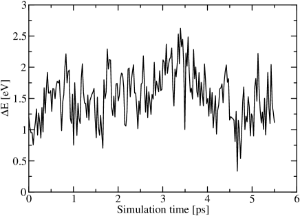
Figure 6: Fluctuations of the vertical energy gap $\Delta E$ for the Ru²⁺-Ru³⁺ electron self-exchange reaction in aqueous solution. The energy gap was calculated according to Eq. 14 for configurations generated with CDFT-MD. See section III for details.

The energy gap Eq. 14 computed for an ensemble of configurations taken from the CDFT-MD trajectory, is shown in Fig. 6 (see section III for computational details). The average is $\langle\Delta E\rangle_{\text{A}}\!=\!1.53$ eV and the mean square fluctuation is $\langle\delta\Delta E^{2}\rangle_{\text{A}}^{1/2}\!=\!0.41$ eV. The error of the average due to the finite length of the trajectory is estimated to be $\approx 0.2$ eV. The probability distribution of the energy gap fluctuations and the corresponding diabatic free energy profile Eq. 15 are shown in Fig. 7. Due to the linear free energy relation Eq. 17 two segments of the free energy curve are obtained from the CDFT-MD equilibrium simulation, one for the equilibrium region, and one for high free energies at the equilibrium region of the product state (see also section II.3 and Refs. Blumberger and Sprik (2006); Blumberger et al. (2006)). The two segments fit well to a parabola with a correlation coefficient of $0.99983$. This shows that the Ru²⁺-Ru³⁺ electron-self exchange is well described in the linear response approximation, which is an essential assumption in Marcus theory of electron transfer.

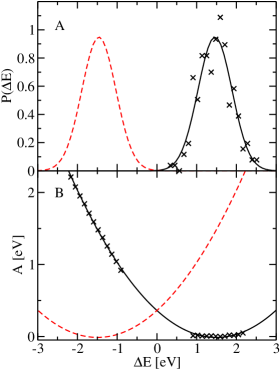
Figure 7: Probability distribution of the energy gap Eq. 14 (A) and diabatic free energy curves Eq. 15 (B) for the Ru²⁺-Ru³⁺ electron self-exchange in aqueous solution. Data points are collected in bins of width $0.11$ eV. The data points in (A) are fit to a Gaussian and reflected about the origin to generate the distribution of the symmetrical product state (dashed lines). In (B) data points within $1.5$ standard deviations from the center of the two distributions are fit to a parabola.

Since for electron self-exchange the reorganization free energy equals the average energy gap (Eq. 16), we obtain $\lambda\!=\!\langle\Delta E\rangle_{\text{A}}=1.53$ eV from CDFT-MD. This value includes the reorganization of the two Ru-hexahydrates and of 51 water molecules solvating the electron transfer complex. Reorganization of higher solvation shells and of bulk solvent is missing. In previous work we have estimated a correction term for reorganization free energy of the missing solvent by carrying out a series of classical molecular dynamics simulations for different system sizes and extrapolating the reorganization free energy obtained to the limit of infinite dilutionBlumberger and Lamoureux (2008). The correction term for the 63 water molecule system amounts to 0.09 eV. Our estimate for reorganization free energy of the infinitely diluted system is then $1.53+0.09\!=\!1.62$ eV. This estimate is within the range of values obtained in previous classical molecular dynamics simulations of the same reaction using polarizable water modelsBlumberger and Lamoureux (2008), 1.60 eV for SWM4-NDP water, 1.71 eV for POL3 water and 1.87 eV for AMOEBA water (values taken from Ref. Blumberger and Lamoureux (2008), corrected for finite size but not for nuclear quantum effects). In a continuum studyRotzinger (2002) a value of 1.95 eV is reported that fits well the experimental rate constant.Bernhard et al. (1985) However, this value was calculated for a Ru-Ru distance of 6.5 Å  and should be corrected to 1.75 eV if the same distance as in the present CDFT-MD simulations is assumed (5.5 Å). Unfortunately a direct experimental estimate for reorganization free energy is not available since the work term and the electronic coupling matrix element are unknownBernhard et al. (1985). Yet, under a number of assumptions, a value of about 2.0 eV was reported in Ref. Bernhard et al. (1985).

V Conclusions and outlook

In this work we have presented an implementation of charge constrained density functional molecular dynamics in the plane-wave code CPMD. Several technical issues of CDFT were investigated such as the dependence of the results on the shape of the weight function used to define the charge constraint. Although for small donor acceptor-distances the energy depends strongly on the weight function, for medium to large distances the dependence is rather small. Thus, it is appealing to use this method for the study of long-range electron transfer problems.

We have demonstrated that it is feasible to calculate electron transfer properties of condensed phase systems within the framework of CDFT-MD. As yet this is not possible with conventional density functional molecular dynamics simulation because for most donor-acceptor systems uncorrected GGA or hybrid density functionals give charge delocalized states for any nuclear configuration. Although the computational cost of CDFT-MD is higher than for standard Born-Oppenheimer dynamics, by a factor of about $2\!-\!3$, CDFT-MD proved to be a viable method for sampling charge-localized diabatic states of condensed phase systems.

The reorganization free energy obtained for aqueous Ru²⁺-Ru³⁺ electron self-exchange, $1.62$ eV, is smaller than estimates reported previously by other authors, $1.95$ eVRotzinger (2002) and $2.0$ eVBernhard et al. (1985). This can be partly explained by the short Ru-Ru distance of $5.5$ Å in our present simulation. Increase of this distance to $6.5$ ÅBrunschwig et al. (1982); Rotzinger (2002) will lead to an increase in reorganization free energy by about 0.2 eV, thus bringing our value closer to previous estimates. However, present CDFT-MD simulations predict that the difference in Ru-O bond lengths in Ru²⁺(H₂O)₆ and Ru³⁺(H₂O)₆ is significantly reduced in the electron transfer complex relative to the isolated aqua ions. Thus, estimation of the inner-sphere contribution from ab-initio calculationsRotzinger (2002) or bond length differencesBrunschwig et al. (1982); Bernhard et al. (1985) of the separated aqua-ions could lead to an overestimation in reorganization free energy, because the deformation of bond lengths in the ET complex are neglected.

In the present work we have focused on the free energy contribution to the electron transfer rate constant. Following Van Voorhis and coworkersWu and Van Voorhis (2006a) we will implement an approximate calculation of the electronic transition matrix element. This will enable us to predict absolute rates for electron or hole transfer in extended systems such as solvated donor-acceptor complexes and solids.

Appendix A Weight function cutoff

The weight function defined in Eq. 9 is always finite even at points in space where all $\rho_{i}$ are zero. Yet, for numerical calculations we introduce for each atom species $k$ a radial cutoff $R_{ck}$ to avoid small numbers in the denominator. This also makes the real space charge integration more efficient. The effect of the cutoff can be formally described by a Heaviside step function $\theta$. Thus, in Eq. 9 we make the following replacement,

$$\rho_{i}(|\mathbf{r}-\mathbf{R}_{i}|)\rightarrow\rho_{i}(|\mathbf{r}-\mathbf{R}_{i}|)\theta(R_{ck}-|\mathbf{r}-\mathbf{R}_{i}|)$$ (19)

where $\mathbf{R}_{i}$ is the position of atom $i$. $R_{ck}$ is chosen such that the total reference density of species $k$ is smaller than $10^{-6}$e, unless stated otherwise.

Appendix B Constraint forces

The additional force on atom $i$ due to the constraint term on the right hand side of Eq. 2 is given by

$$\mathbf{F}_{\text{c}i}=-V\int\rho(\mathbf{r})\frac{\partial w(\mathbf{r},\mathbf{R})}{\partial\mathbf{R}_{i}}\;d\mathbf{r}.$$ (20)

For the weight function defined in Eq. 12 the derivative in the integrand of Eq. 20 is given by

$$\frac{\partial w(\mathbf{r},\mathbf{R})}{\partial\mathbf{R}_{i}}=-\frac{\rho_{i}^{\prime}(|\mathbf{r}-\mathbf{R}_{i}|)}{\sum_{j=1}^{N}\rho_{j}(|\mathbf{r}-\mathbf{R}_{j}|)}G_{i}(\mathbf{r}-\mathbf{R}_{i})$$ (21)

where

$$G_{i}(\mathbf{r}-\mathbf{R}_{i})=\left\{\begin{array}[]{l c r}w(\mathbf{r}-\mathbf{R}_{i})-1&&i\in D\\ w(\mathbf{r}-\mathbf{R}_{i})+1&&i\in A\\ w(\mathbf{r}-\mathbf{R}_{i})&&i\not\in D\cup A\\ \end{array}\right.$$ (25)

depending on whether atom $i$ is in the group of donor (D) or acceptor (A) atoms, or in neither of them (e.g. solvent atoms). The derivative of the density is given by

$$\rho_{i}^{\prime}(|\mathbf{r}-\mathbf{R}_{i}|) = \frac{\partial\rho_{i}(|\mathbf{r}-\mathbf{R}_{i}|)}{\partial\mathbf{R}_{i}}$$ (26)

$$= \frac{\partial\rho_{i}(|\mathbf{r}-\mathbf{R}_{i}|)}{\partial|\mathbf{r}-\mathbf{R}_{i}|}\frac{\mathbf{r}-\mathbf{R}_{i}}{|\mathbf{r}-\mathbf{R}_{i}|}.$$

The radial partial derivative of $\rho_{i}$ is calculated numerically using splines. However, due to the radial cutoff of the density (Eq. 19) the derivative Eq. 26 has to be replaced as follows,

$$\rho_{i}^{\prime}(|\mathbf{r}-\mathbf{R}_{i}|) \rightarrow \rho_{i}^{\prime}(|\mathbf{r}-\mathbf{R}_{i}|)\theta(R_{ck}-|\mathbf{r}-\mathbf{R}_{i}|)$$ (27)

$$+ \rho_{i}(|\mathbf{r}-\mathbf{R}_{i}|)\delta(R_{ck}-|\mathbf{r}-\mathbf{R}_{i}|),$$

where $\delta$ is the Dirac delta function. Thus, the constraint force, Eq. 20, is composed of two terms, the force due to $w$ within $R_{ck}$, $\mathbf{F}_{ci}^{\text{inside}}$, and a surface term, $\mathbf{F}_{ci}^{\text{surf}}$,

$$\mathbf{F}_{ci}=\mathbf{F}_{ci}^{\text{inside}}+\mathbf{F}_{ci}^{\text{surf}}$$ (28)

where

$$\mathbf{F}_{ci}^{\text{inside}} = \!\!-V\!\!\int\!\!\rho(\mathbf{r})\frac{\partial w(\mathbf{r},\mathbf{R})}{\partial\mathbf{R}_{i}}\;\theta(R_{ck}-|\mathbf{r}-\mathbf{R}_{i}|)\;d\mathbf{r}$$ (29)

$$\mathbf{F}_{ci}^{\text{surf}} = -V\rho_{i}(R_{ck})R_{ck}\int\frac{\rho(R_{ck},\vartheta,\varphi)G(R_{ck},\vartheta,\varphi)}{\sum\rho_{i}(R_{ck},\vartheta,\varphi)}$$ (33)

$$\times R_{ck}\left(\begin{array}[]{c}\sin\vartheta\cos\varphi\\ \sin\vartheta\sin\varphi\\ \cos\vartheta\end{array}\right)\sin\vartheta\;d\vartheta d\varphi$$

The derivative in the integrand of Eq. 29 is given by Eqs. 21-26 and in Eq. 33 we have changed to spherical coordinates. The surface force Eq. 33 is integrated over a thin shell on a cartesian grid. $R_{ck}$ times the radial unit vector is just the position vector of a point on the surface $(x,y,z)$. Thus the surface element can be expressed in cartesian coordinates as

$$\sin\vartheta\;d\vartheta d\varphi=\operatorname{sgn}(z)\frac{y\;dxdz-x\;dydz}{R_{ck}(R_{ck}^{2}-z^{2})}$$ (34)

Appendix C Prediction of the Lagrange multiplier $V$ in CDFT-MD

In a deterministic Born-Oppenheimer MD simulation the ionic positions and momenta at any given timestep depend on the configurations at earlier times such that – using a suitable algorithm – one can calculate the evolution of the system in time. The Lagrange multiplier $V$ used in the calculation of the constrained energy functional Eq. 2 is in principle an unknown function of all ionic positions. However, the positions change smoothly during the dynamics. Thus, one can devise an algorithm for prediction of $V(t)$ from the history of $V$. This should provide a better initial guess for the search of the unknown Lagrange multiplier. We chose a Lagrange polynomial of order $n$ for this purposeBronstein et al. (1999):

$$V(t_{k+1})=\sum_{j=k-n}^{k}V(t_{j})\prod_{i=k-n,i\neq j}^{k}\frac{t_{k+1}-t_{i}}{t_{j}-t_{i}}$$ (35)

where $k$ is the index of the last timestep. In Eq. 35 information from $n$ timesteps preceding step $k$ is used to extrapolate the value of $V$ for timestep $k+1$. Naively, one would expect higher order polynomials to perform better. Yet we found for CDFT-MD simulation of the aqueous Ru²⁺-Ru³⁺ complex (section IV.5) an optimum extrapolation order of $n=2$. Higher order polynomials led to an oscillatory behaviour of Eq. 35 and to poor initial guess values. We note that the optimal order for extrapolation of $V$ depends very much on the system under consideration. Therefore it seems advisable to calculate the optimum interpolation order for each system in advance from a short test-run before carrying out simulations on a larger scale.