Atomistic theory for the damping of vibrational modes in mono-atomic gold chains

Abstract

We develop a computational method for evaluating the damping of vibrational modes in mono-atomic metallic chains suspended between bulk crystals under external strain. The damping is due to the coupling between the chain and contact modes and the phonons in the bulk substrates. The geometry of the atoms forming the contact is taken into account. The dynamical matrix is computed with density functional theory in the atomic chain and the contacts using finite atomic displacements, while an empirical method is employed for the bulk substrate. As a specific example, we present results for the experimentally realized case of gold chains in two different crystallographic directions. The range of the computed damping rates confirm the estimates obtained by fits to experimental data [Frederiksen et al., Phys. Rev. B 75, 205413(R)(2007)]. Our method indicates that an order-of-magnitude variation in the harmonic damping is possible even for relatively small changes in the strain. Such detailed insight is necessary for a quantitative analysis of damping in metallic atomic chains, and in explaining the rich phenomenology seen in the experiments.

I Introduction

The continuing shrinking of electronic devices and the concomitant great interest in molecular electronicsCuniberti et al. (2005) have underlined the urgency of a detailed understanding of transport of electrons through molecular-scale contacts. A particularly important issue concerns the energy exchange between the charge carriers and the molecular contact. Thus, the local Joule heating resulting from the current passing through the contact, and its implications to the structural stability of such contacts are presently under intense investigationSchulze et al. (2008); Teramae et al. (2008); Huang et al. (2007); Galperin et al. (2007); Ryndyk et al. (2008). Experimentally, local heating in molecular conductors in the presence of the current has been inferred using two-level fluctuationsTsutsui et al. (2008a) and Raman spectroscopyIoffe et al. (2008).

Mono-atomic chains of metal atomsRubio-Bollinger et al. (2001) are among the simplest possible atomic-scale conductors. The atomic gold chain is probably the best studied atomic-sized conductor, and a great deal of detailed information is available from experimentsRodrigues and Ugarte (2001a); Agraït et al. (2002a, b); Legoas et al. (2002); Agraït et al. (2003); Rego et al. (2003); Coura et al. (2004); Bettini et al. (2005); Lagos et al. (2007); Hasmy et al. (2008); Kizuka (2008); Thiess et al. (2008); Tsutsui et al. (2008b), and related theoretical studiesTodorov (1998); Bahn and Jacobsen (2001); da Silva et al. (2001); Legoas et al. (2002); Rego et al. (2003); Chen et al. (2003); Montgomery et al. (2003); Frederiksen et al. (2004); Viljas et al. (2005); Paulsson et al. (2005); Frederiksen et al. (2007a, b); Lagos et al. (2007); Hobi et al. (2008). The current induced vibrational excitation and the stability of atomic metallic chains have been addressed in a few experimentsYasuda and Sakai (1997); Smit et al. (2004); Tsutsui et al. (2005, 2006).

In the case of a gold chain Agraït et al.Agraït et al. (2002b) reported well-defined inelastic signals in the current-voltage characteristics. These signals were seen as a sharp 1% drop of the conductance at the on-set of back-scattering due to vibrational excitation when the voltage equals the vibrational energy. Especially for the longer chains (6-7 atoms), the vibrational signal due to the Alternating Bond-Length (ABL) modeFrederiksen et al. (2004); Frederiksen et al. (2007a), dominates. This resembles the situation of an infinite chain with a half-filled electronic band where only the zone-boundary phonon can back-scatter electronsAgraït et al. (2002a) due to momentum conservation.

The inelastic signal gives a direct insight into how the frequency of the ABL-mode depends on the strain of the atomic chain. This frequency can also be used to infer the bond strength. The signature of heating of the vibrational mode is the non-zero slope of the conductance versus voltage beyond the on-set of excitation: with no heating the curve would be flat. Fits to the experiment on gold chains using a simple modelPaulsson et al. (2005) suggest that the damping of the excitation, as expected, can be significant. However, the experiments in general show a variety of behaviors and it is not easy to infer the extent of localization of the ABL vibration or its damping in these systems .

In order to address the steady-state effective temperature of the biased atomic gold chain theoretically, it is necessary to consider the various damping mechanisms affecting the localized vibrations, such as their coupling to the vibrations in the contact, or to the phonons in the surrounding bulk reservoirs. This is the purpose of the present paper: we calculate the vibrational modes in atomic gold chains and their coupling and the resulting damping due to the phonon system in the leads. We work within the harmonic approximation and employ first principles density functional theory (DFT) for the atomic chain and the contactsSoler et al. (2002) while a potential model is used for the force constants of the leadsTr glia and Desjonqu res (1985).

Experimental TEM studiesRodrigues and Ugarte (2001b); Kizuka (2008) have shown that atomic chains form in the $\langle 100\rangle$ and $\langle 111\rangle$ directions while the $\langle 110\rangle$ direction gives rise to thicker rodsRodrigues and Ugarte (2001b). Therefore we focus on chains between two (100)-surfaces or (111)-surfaces. We consider chain-lengths of 3-7 atoms and study the behavior of their vibrations and damping when the chains are stretched. The TEM micrographs also indicate that the chains are suspended between pyramids, so in our calculations we add the smallest possible fcc-stacked pyramid to link the chain to the given surfaces.

As we shall show below, at low strain the gold chains have harmonically undamped ABL-modes with frequencies outside the bulk band. The long chains of 6-7 atoms also have ABL-modes with very low damping at high strain . Our results indicate that chains between (111)-surfaces will have a lower damping than chains between (100)-surfaces. Importantly, we find that the damping is an extremely sensitive function of the external strain: an order of magnitude change may result from minute changes in the strain. This may provide a key for understanding the rich behavior found in experiments.

The paper is organized as follows. In Sect. II we describe how the central quantities, i.e., the dynamical matrix, the projected density-of-states, and the damping rates are calculated. Section III is devoted to the analysis of the numerical results we have obtained, beginning with results for the structure of the chains, proceeding to the dynamical matrix, and concluding with an analysis of the damping of modes in the systems. Section IV gives our final conclusions, while certain technical details are presented in three appendices.

II Method

Figure 1: Two ways of partitioning the central part of the chain-substrate system. [Top] The Chain is the part of the system that only contains one atom in a plane parallel to the surface, and the Base is what connects the two-dimensional surface to the Chain. [Bottom] The Pyramid is the Base plus the Chain atom closest to the Base. The Central Chain is the remaining part of the Chain after removing one atom at each end.

As will become evident in the forthcoming discussion it is advantageous to use two different ways to label the atoms forming the junction; these two schemes are illustrated in Fig. 1. The first scheme (Fig. 1 top panel) is based on the cross-sectional area and collects all atoms with equilibrium positions on the one-dimensional line joining the two surfaces into a "Chain", and calls the remaining atoms between the Chain and the substrate the "Base". The second scheme (Fig. 1, bottom) distinguishes between a "Pyramid" and a "Central Chain"; this is chosen because the last atom of the Chain has bonds to four or five atoms making this atom very different from the Central Chain atoms that only have two bonds per atom.

A quantity of central importance to all our analysis is the mass-scaled dynamical matrix, K, which we here define as including $\hbar$,

$$\textbf{K}_{ij}=\frac{\hbar^{2}}{\sqrt{m_{i}m_{j}}}\frac{\partial^{2}E}{\partial u_{i}\partial u_{j}}\quad,$$ (1)

where $E$ is the total energy of the system, $u_{i}$ is the coordinate corresponding to the $i$’th degree of translational freedom for the atoms of the system. $m_{i}$ is the mass of the atom that the $i$’th degree freedom belongs to. K governs the the evolution of the vibrational system within the harmonic approximation. In the Fourier domain the Newton equation of motion reads

$$\textbf{K}u_{\lambda}=\epsilon^{2}_{\lambda}u_{\lambda}\quad,$$ (2)

where $\lambda$ denotes a mode of oscillation in the system and $\epsilon_{\lambda}$ is the corresponding quantization energy.

The evaluation of K proceeds as follows. Finite difference DFT calculations (for details of our implementation, see App. A) were used for the Chain, the Base and the coupling between the surface and the Base while for the surfaces we used an empirical model due to Tr glia and Desjonqu resTr glia and Desjonqu res (1985). Figure 2 illustrates the domains for the two different methods. The position of the interface between the region treated by DFT and the region treated by the empirical model is a parameter that can be varied, and the dependence on the final results of the choice of this parameter is analyzed in App. B.2.

Figure 2: Parameters used for calculating the dynamical matrix. Only nearest-neighbor coupling is shown. The coupling elements labeled ’EM’ are found by the empirical model and the coupling elements labeled ’DFT’ by DFT. On-site elements are determined from the coupling elements (see Sec. A) and are not shown in the figure.

The empirical model can be used to describe the on-site and coupling elements of atoms in a crystal structure. The model uses the bulk modulus of gold to fit the variation in the force constant with distance between nearest and next-nearest neighbors. Even though the empirical model is fitted to the bulk modulus, which is a low frequency property, it still accurately predicts the cutoff of the bulk band. The positions of the neighboring atoms can only have small deviations from perfect crystal positions (eg. bulk, surface and ad-atoms). Note that this model is general enough to give different coupling elements between surface atoms and bulk atoms. The model also distinguishes between the coupling between surface atoms with or without extra atoms added to the surface.

The DFT calculations were done with the SIESTA code, using the Perdew-Burke-Enzerhof version of the GGA exchange-correlation potential with standard norm-conserving Troullier-Martins pseuodopotentials. We used an SZP basis set with a confining energy of $0.01~{}\textrm{Ry}$. A mesh cutoff of $150~{}\textrm{Ry}$ was used. Relaxation was done with a force tolerance of $0.002~{}\textrm{eV}/\textrm{\AA}$. These values were found to have converged for the same type of system by Frederiksen et al.Frederiksen et al. (2007a, b). The experimental fcc bulk lattice constant of $4.08~{}\textrm{\AA}$ was used. Only the device region was relaxed (defined in Fig. 3).

For the (111) orientations a 4$\times$4 atom surface unit and a 2$\times$3 $k$-point sampling was used, while for the (100) orientations a 3$\times$3 atom surface unit cell and a 3$\times$3 $k$-point sampling was employed. This ensured a similar and sufficient $k$-point density for both kinds of surfaces (see App. B.2).

II.1 Green’s function for a perturbation on the surface

All properties of interest in the present context can be derived from the (retarded) Green’s function D, defined by

$$[(\epsilon+i\eta)^{2}\textbf{I}-\textbf{K}]\textbf{D}(\epsilon)=\textbf{I}\equiv\textbf{M}\textbf{D}\quad,$$ (3)

where $\eta=0^{+}$ and we defined the inverse of the Green’s function by $\textbf{M}=\textbf{D}^{-1}$. Specifically, we shall need the Green’s function projected onto the region close to the Chain. Our procedure is based on a method due to Mingo et al.Mingo et al. (2008) which has previously been tested in an investigation of finite Si nanowires between Si surfaces. We define $\textbf{X}_{YZ}$ as the the block of the matrix X, where the indices run over the degrees of freedom in regions $Y,Z$, respectively, where $Y,Z=\{1,2,A,D,L,R\}$, as defined either in Fig. 1 or Fig. 3.

Figure 3: Adding atoms to two surfaces. [Top] The forces between surface atoms within next-nearest neighbor distance(4.08Å) of the added atoms are perturbed by the presence of the added atoms. [Bottom] The device region is where the coupling between the atoms is different from the values for the two unperturbed surfaces. The coupling between the device region and the leads is considered to be unperturbed.

First, let us start with two perfect surfaces. We then add the atoms that connect these surfaces (the Base and the Chain). Within a certain range from the added atoms the on-site and coupling elements of K will be different from the values for the perfect surface. Together, the added atoms and the perturbed atoms define the device region $D$ (Fig. 3, bottom). The coupling between the device region and the rest of the surface ($L,R$ for the left and right leads, respectively) is assumed to be unperturbed.

In order to compute the Green’s function projected on the device region, $\textbf{D}_{DD}(\epsilon)$, we first consider this matrix representation of Eq. (3):

$$\left(\begin{array}[]{cc}\textbf{M}_{DD}&\textbf{M}_{D\alpha}\\ \textbf{M}_{\alpha D}&\textbf{M}_{\alpha\alpha}\\ \end{array}\right)\left(\begin{array}[]{cc}\textbf{D}_{DD}&\textbf{D}_{D\alpha}\\ \textbf{D}_{\alpha D}&\textbf{D}_{\alpha\alpha}\\ \end{array}\right)=\left(\begin{array}[]{cc}\textbf{I}_{DD}&\textbf{0}_{D\alpha}\\ \textbf{0}_{\alpha D}&\textbf{I}_{\alpha\alpha}\\ \end{array}\right).$$ (4)

Here the index $\alpha=(L,R)$, i.e., the left and right unperturbed surface, while $D=\{1,A,2\}$. Using straightforward matrix manipulations one finds

$$\textbf{D}_{DD} = [\textbf{M}_{DD}-\textbf{M}_{D\alpha}(\textbf{M}_{\alpha\alpha})^{-1}\textbf{M}_{\alpha D}]^{-1}$$ (5)

$$= [\textbf{M}_{DD}-\bm{\Pi}_{DD}]^{-1}\quad,$$

which defines the self-energy $\bm{\Pi}_{DD}=\textbf{M}_{D\alpha}(\textbf{M}_{\alpha\alpha})^{-1}\textbf{M}_{\alpha D}$. Since the added atoms do not couple to the unperturbed surfaces, and the perturbed region 1 couples only to the right unperturbed surface while the perturbed region 2 only couples to the left unperturbed surface, the self-energy $\bm{\Pi}_{DD}$ has the matrix structure

$$\bm{\Pi}_{DD}=\left(\begin{array}[]{ccc}\textbf{M}_{1L}(\textbf{M}_{LL})^{-1}\textbf{M}_{L1}&0&0\\ 0&0&0\\ 0&0&\textbf{M}_{2R}(\textbf{M}_{RR})^{-1}\textbf{M}_{R2}\\ \end{array}\right).$$ (6)

This object can be evaluated as follows. First, in the limit of large regions 1 and 2, the coupling elements $\textbf{M}_{L1}$ and $\textbf{M}_{R2}$ must approach those of the unperturbed surface, $\textbf{M}^{S}_{L1}$ and $\textbf{M}^{S}_{R2}$, respectively. In what follows, we shall make the approximation that the regions 1 and 2 are chosen so, that this condition is satisfied sufficiently accurately. Second, we note that the matrix $\textbf{M}_{\alpha\alpha}$ is indistinguishable from the matrix $\textbf{M}^{S}_{\alpha\alpha}$, as long as the involved atoms are outside the perturbed regions 1 or 2. Therefore, we can write

$$\textbf{M}_{1L}(\textbf{M}_{LL})^{-1}\textbf{M}_{L1} \simeq \textbf{M}^{S}_{1L}({\textbf{M}^{S}_{LL}})^{-1}\textbf{M}^{S}_{L1}\equiv\bm{\Pi}^{S}_{11}$$

$$\textbf{M}_{2R}(\textbf{M}_{RR})^{-1}\textbf{M}_{R2} \simeq \textbf{M}^{S}_{2R}({\textbf{M}^{S}_{RR}})^{-1}\textbf{M}^{S}_{R2}\equiv\bm{\Pi}^{S}_{22},$$

where the accuracy increases with increasing size of regions 1 and 2. On the other hand, using the definition of the self-energy, we can write

$$\bm{\Pi}^{S}_{11} = \textbf{M}^{S}_{11}-(\textbf{D}^{S}_{11})^{-1}$$

$$\bm{\Pi}^{S}_{22} = \textbf{M}^{S}_{22}-(\textbf{D}^{S}_{22})^{-1},$$ (8)

where $\textbf{D}^{S}_{ii},i=1,2$ is the projection of the unperturbed Green’s functions onto the atoms in regions 1,2, respectively. This object is evaluated by exploiting the periodicity in the ideal surface plane. The Fourier transform of $\textbf{M}^{S}$ in the parallel directions has a tridiagonal block structure and we can solve for its inverse very effectively using recursive techniques (see e.g. Sancho et al.Sancho et al. (1984)). Of course we still have to evaluate the Fourier transform for a large number of $k$-points. The density of $k$-points as well as the size of the infinitesimal $\eta$ are convergence parameters which determine the accuracy and cost of the computation. An analysis of the choice of these parameters is given in App. B.2.

To sum up, the calculation is preformed in the following steps: (i) Start with perfect leads and specify the device in between them. (ii) The atoms in the leads where K is perturbed by the presence of the device are identified. (iii) The unperturbed surface Green’s function $\textbf{D}^{S}$ is found via $k$-point sampling and then used to construct the self-energy, Eqs.(II.1–II.1). (iv) The perturbed Green’s function is then found using this self-energy via Eqs.(5–6).

II.2 Modes and life-times

For any finite system the eigenvalues $\epsilon_{\lambda}^{2}$ and thereby also the density of states are found straightforwardly. For infinite systems we use that each eigenvector, $u_{\lambda}$, with the corresponding eigenvalue, $\epsilon_{\lambda}$ gives a contribution to the imaginary part of the Green’s function in the $\epsilon_{\lambda}\gg\eta$ limit

$$u_{\lambda}^{\dagger}\mathrm{Im}\textbf{D}(\epsilon)u_{\lambda}\approx-\frac{1}{2\epsilon_{\lambda}}\frac{1}{(\epsilon-\epsilon_{\lambda})^{2}+\eta^{2}}.$$

This expression results in the following density of states

$$\textbf{n}(\epsilon)=-\frac{2\epsilon}{\pi}\lim_{\eta\rightarrow 0^{+}}\mathrm{Im}\textbf{D}(\epsilon).$$ (9)

The broadened vibrational modes of the device region can each be associated with a finite life-time. To do this we need to have a definition of an approximate vibrational mode of the central part of the system that evolves into an eigenmode of K when the coupling to the leads tends to zero. We define ’modes’ as the vectors that for some energy, $\epsilon^{*}$, correspond to a zero eigenvalue mode of $\mathrm{Re}\textbf{D}_{DD}(\epsilon^{*})$ (see Sec. C for details).

We also need to define a few characteristics of a mode. The Green’s function projected onto a mode can be approximated by a broadened free phonon propagator with constants $\epsilon_{\lambda}$ and $\gamma_{\lambda}$ in a neighborhood of the mode peak energy,

$$u_{\lambda}^{\dagger}\textbf{D}_{DD}(\epsilon)u_{\lambda} = \frac{1}{(\epsilon+i\gamma_{\lambda})^{2}-\epsilon_{\lambda}^{2}}$$

$$= \frac{1}{\epsilon^{2}-(\epsilon_{\lambda}^{2}+\gamma_{\lambda}^{2})+i2\epsilon\gamma_{\lambda}}\quad.$$

The time-dependent version of the Green’s function is an exponentially damped sinusoidal oscillation with damping rate of $\frac{\gamma_{\lambda}}{\hbar}$, mean life-time, $\tau_{\lambda}=\frac{\hbar}{\gamma_{\lambda}}$, and $Q$-factor, $Q_{\lambda}=\frac{\epsilon_{\lambda}}{2\gamma_{\lambda}}$. Comparing the broadened phonon propagator to Eq. (5) we see that $u_{\lambda}^{\dagger}\mathrm{Im}\bm{\Pi}(\epsilon)u_{\lambda}=-2\epsilon\gamma_{\lambda}$, leading to

$$\gamma_{\lambda}=-\frac{u_{\lambda}^{\dagger}\mathrm{Im}\bm{\Pi}(\epsilon^{*})u_{\lambda}}{2\epsilon^{*}}\quad,$$

where $\epsilon^{*}$ is the the mode peak energy.

This calculation of $\gamma_{\lambda}$, $Q_{\lambda}$ and $\tau_{\lambda}$ only strictly makes sense for peaks with a Lorentzian line shape. This requires that $u_{\lambda}^{\dagger}\mathrm{Im}\textbf{D}_{DD}(\epsilon)u_{\lambda}$ is approximately constant across the peak which is the case for modes with small broadening and large life-time. Nevertheless, we will also use these definitions for the delocalized modes since the calculated values are still a measure of interaction with the leads.

We also define a measure of spatial localization, $s_{\lambda}$,

$$s_{\lambda}=\frac{\sum_{x\in C}|(u_{\lambda})_{x}|^{2}}{\sum_{x\in D\backslash C}|(u_{\lambda})_{x}|^{2}}\frac{N_{D}-N_{C}}{N_{C}}\quad,$$

where $N_{D}$ and $N_{C}$ are the number of atoms in the device and central chain region respectively and $D\backslash C$ means Device region except the Central Chain (the perturbed reigion). This quantity is useful to pick out modes with a large amplitude in the Central Chain region only. We have that $s_{\lambda}=1$ signifies equal amplitude in $C$ and connecting atoms, while the limit $s_{\lambda}\rightarrow\infty$ ($s_{\lambda}\rightarrow 0$) signifies a mode which is completely residing inside(outside) the Chain.

It should be stressed that the mode properties calculated in this way only refer to the harmonic damping by the leads and that other sources of damping are not included such as electron-hole pair creation and anharmonicity. The damping due to electron-hole pair creation, obtained by an ab-initio calculation on a selection of gold chains, is about $50-80~{}\textrm{$\mu$eV}$ for the vibrational mode with the strongest coupling to electronsPaulsson et al. (2005); Frederiksen et al. (2007a). This type of damping is less dependent on strain in gold chains due to stable electronic structure as evidenced by the robust electronic conductance of one conductance quantum. The harmonic damping due to the leads is typically higher than this, but as we shall see it can actually drop well below this value and thus be less than the electron-hole pair damping.

In case of an applied bias the high frequency modes may be excited to a high occupation. The creation of vibrational quanta is roughly proportional to $eV-\hbar\omega_{\lambda}$, while the damping mechanisms are not expected to have a strong dependence of the bias. Therefore, as the bias is increased beyond the phonon energy threshold, the mode occupation will rise and anharmonic interactions may become increasingly important even for low temperatures. MingoMingo (2006) has studied anharmonic effects on heat-conduction in a model atomic contact, and more recently Wang and co-workerset al.Wang et al. (2008) has used ab-initio calculations to access the effect of anhamonicity on heat-conduction in carbon-based systems. Anharmonic effects are, however, outside the scope of the present work.

III Results

III.1 Geometrical Structure and the Dynamical Matrix

In this subsection we investigate the geometrical structure of the chains and the behavior of the dynamical matrix. For each type of calculation (identified by the number of atoms in the Chain, the surface orientation and the type of Base) a range of calculations were set up with the two surfaces at different separations, $L_{i}\,(i=1,2...)$, with the separations incremented in equally spaced steps. Trial-and-error was used to determine suitable step sizes for the different types of calculations.

To be able to compare chains of different lengths and between different surfaces we define the average bond length, $B=\langle b_{j}\rangle$, as the average length between neighboring atoms within the Chain, where $j$ runs over the number of bonds in the Chain (see Fig. 4). $B$ is useful because it is closely related to the experimentally measurable forceAgraït et al. (2003) on the Chain and can be found without interpolation. The close relationship between $B$ and the force is demonstrated in Fig. 5 where the force is calculated as the slope of a least-squares fit of

$$[(E_{i-1},L_{i-1}),(E_{i},L_{i}),(E_{i+1},L_{i+1})]$$

where $E$ is the total energy. We note that the force vs. $B$ curves to a good approximation follows a straight line with a slope of $k=2.5~{}\textrm{eV}/\textrm{\AA}^{2}$, which can be interpreted as the spring constant of the bonds in the Chain. In addition to $B$ we also define the average bond angle $T=\langle\theta_{j}\rangle$.

Figure 4: Distances and angles used to define the average bond length, $B=\langle b_{j}\rangle$, and the average bond angle, $T=\langle\theta_{j}\rangle$, respectively

The behavior of the systems with respect to $B$ is relatively simple. As the systems are strained it is mostly the bonds in the chain that are enlongated. Finally the central bond(s) become so weak that they break. At low $B$ we see from Fig. 6 that the longer chains adopt a zig-zag confirmation at low average bond length. The 3- and 4-atom chains, however, remain linear within the investigated range. Furthermore, the longer chains have a similar variation in the average bond angle.

These preliminary observations are in agreement with previous theoretical studies by Frederiksen et al.Frederiksen et al. (2007a) and Sánchez-Portal et al.Sánchez-Portal et al. (1999). We recount these observations because we find that using $B$ as a parameter provides a helpful way to compare chain of different lengthts and because the calculations in this paper are the most accurate to date.

Figure 5: (color online) Force as function of average bond length, $T=\langle\theta_{j}\rangle$.

Figure 6: (color online) Average bond angle as a function of the average bond length. The long chains adopt a zig-zag structure at low $B$ while the short chains remain linear.

To shed light on the effect of straining the chains, we next investigate the energies that are related to different types of movement by analyzing the eigenmodes and eigenvalues of selected blocks of K. Especially, we can consider the local motion of individual atoms or groups of atoms, freezing all other degrees of freedom, by picking the corresponding parts of K. For a single atom this amounts to the on-site $3\times 3$ blocks. The square root of the positive eigenvalues of the reduced matrix, which we call local energies, give the approximate energy of a solution to the full K that has a large overlap with the corresponding eigenmode, if the coupling to the rest of the dynamical matrix is low. The negative eigenvalues of a block are ignored since they correspond to motion that is only stabilized by degrees of freedom outside the block.

The behavior of the dynamical matrix in terms of local energies, is relatively straightforward, as illustrated in Fig. 7. When the bonds are strained they are also weakened. In the Central Chain the local energies are quickly reduced with increased strain ($\approx 65\%$ decrease) while the dynamical matrix of the surfaces is hardly affected. The Base and the first atom of the Chain fall in between these two extremes with a $20\%$ and $40\%$ decrease, respectively. The middle bonds in the Central Chain are the ones that are strained and weakened the most when the surfaces are moved apart. It is also where the chain is expected to breakVelez et al. (2008). Most interestingly, we note that at least one jump in the on-site local energies occur when moving from the Surface to the Central Chain.

In Fig. 8 we see how motion parallel to the chain is at higher energies than perpendicular motion, and that the LO type motion of the ABL modes has the highest energy. We also see that the local energies of the ABL/LO type motion moves past the local energies of the Pyramid as the strain is increased. In this way the ABL/LO modes can in some sense act as a probe of the contacts.

Figure 7: (color online) Local energies of a 4 atom chain between two (100)-surfaces at different strains. The largest eigenvalues are connected by a line to guide the eye.

Figure 8: Local energies for selected blocks of K (Pyramid/Central Chain) plotted vs. the average bond length in the 4 atom chain. Since the central chain in this case consists of 2 atoms we can classify the eigenvectors as LO: longitudinal optical, LA: longitudinal acoustic, TO: transverse optical (doubly degenerate) or TA: transverse acoustic (doubly degenerate).

III.2 Mode life-times and $Q$-factors

We next investigate the modes of the finite chain systems. An example is given in Fig. 9 which depicts the projected DOS for a chain with 4 atoms at an intermediate strain. Notice the large variation in the width of the peaks. The peaks with a low width correspond to modes that have the largest amplitude in the Chain, while the peaks with a large width correspond to modes with large amplitude on the Base and Surface. Since this type of system has no natural boundary between ’device’ and ’leads’ we will have large variation in the harmonic damping no matter where we define such a boundary.

Figure 9: Projected DOS onto a representative selection of the vibrational modes of the device region that has a large overlap with the added (Chain+Base) region.

In Fig. 10 we present the $Q$-factor, spatial localization and peak energy of all modes for chains with 3-7 atoms between (100) surfaces. These are the main result of this article. Table 1 shows the same information in an alternative form. We now proceed to an analysis of these results.

The ABL modes are of special interest. These modes have been identified by previous theoretical and experimental studies as the primary scatterers of electronsAgraït et al. (2002b); Frederiksen et al. (2004); Frederiksen et al. (2007b); Viljas et al. (2005); Paulsson et al. (2005); Hobi et al. (2008); Hihath et al. (2008). The ABL modes are easily identified in Fig. 10 since they have the highest energy of the modes that are spatially localized to the central chain (black or dark gray on the figure). Modes corresponding to transverse motion of the central chain are also clearly visible. These modes are energetically and spatially localized, but are of limited interest because of a low electron-phonon coupling.

Certain ABL modes are very long-lived. At low strains, ABL modes lie outside the bulk (and surface) band and have, in our harmonic approximation, an infinite $Q$-factor. In reality the $Q$-factor will be limited by electron-phonon and anharmonic interactions. At higher strain the ABL modes move inside the bulk band and one observes a great variation in the corresponding $Q$-factors. When the peak energy lies inside the bulk band there exists modes in the bulk with the same energy and it will mostly be the structure of the connection between the bulk crystal and the chain that determines the width of the peak.

The long chains tend to have longer lived ABL/LO modes due to the larger ratio between the size of the Central Chain and the size of its boundary. The 7-atom chain is especially interesting since it has an ABL/LO type mode with a damping of $5~{}\textrm{meV}$ at one strain, while at another strain the ABL/LO mode has a damping of 300 meV, i.e., more than one order-of-magnitude variation in the harmonic damping of the primary scatterer of electrons due to only a 0.03 Å change in the average bond length!

The largest damping of an ABL-mode for these systems is $\gamma_{\lambda}\approx 1~{}\textrm{meV}$, which is still significantly lower than the $\approx 20~{}\textrm{meV}$ band width. This can be attributed to fact, noted above, that there always exists a large mismatch in local energies moving from the central part of the chain to the rest of the system (see Fig. 7).

Previous studies by Frederiksen et al.Frederiksen et al. (2007a) obtained a rough estimate for the variation of the non-electronic(harmonic and anharmonic) damping of 5-50 $\mu$eV for the longer chains by fitting the experimental IETS signals of Agraït et al.Agraït et al. (2002a) to a model calculation. The estimated peak energies lie well within the bulk band for all the recorded signals. The reason the non-electronic damping rate can be extracted is because the excitation of vibrations and damping of vibrations through electron-hole creation are both proportional to the strength of the electron-phonon coupling. This means that the step in the experimental conductance, when the bias reaches the phonon energy, can be used to estimate strength of the electron-phonon interaction and thereby the electron-hole pair damping. The slope in the conductance beyond this step can then be used to extract the total damping. By subtracting the electron-hole pair damping from the total damping we get an estimate of the sum of the sum of harmonic and anharmonic contributions to the damping.

The estimate in Ref. [Frederiksen et al., 2007a] agrees well with our lowest damping of 5 $\mu$eV. The highest damping we have found was $\approx 400~{}\textrm{$\mu$eV}$ found for the 6 atom chain which is an order of magnitude larger than the upper limit of Ref. [Frederiksen et al., 2007a]. We believe that this discrepancy can be largely attributed to the difficulty in extracting the necessary parameters from experiments when the harmonic damping is large. Furthermore, for the 6-7 atom chains we observe that the high damping occurs at low strain, where the electron-phonon coupling is weakAgraït et al. (2002a).

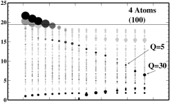
Figure 10: The vibrational modes for chains with 3-7 atoms between two 100-surfaces. The center of the disks are positioned at the peak of the projection of vibrational DOS on the mode in question. The area of a disk is proportional to the $Q_{\lambda}$, but is limited to what corresponds to a $Q$-factor of 250. he gray level, that ranges from light gray to black in 4 steps signifies that $s_{\lambda}\in[0,2[\text{(light gray)},[2,4[,[4,6[,[6,8[$ or $[8,\infty[$(black).

Figure 11: The vibrational modes for 5 atom chains between two (111) surfaces. [Top] Symmetric pyramids. [Bottom] Asymmetric pyramids (one atom added to one of the pyramids). The area of a disk is proportional to the $Q_{\lambda}$, but is limited to what corresponds to a $Q$-factor of 250. The gray level, that ranges from light gray to black in 4 steps signifies that $s_{\lambda}\in[0,2[\text{(light gray)},[2,4[,[4,6[,[6,8[$ or $[8,\infty[$(black).

Chain	$Q_{\lambda}$	$\gamma_{\lambda}$($\mu$eV)	$\tau_{\lambda}$(ps)
3(100)	3-7	800-1200	0.5-0.8
4(100)	5-30	100-900	0.7-7
5(100)	10-40	200-500	1.3-3
6(100)	15-80	90-400	1.6-7
7(100)	40-1500	5-300	2-130
5(111)(symmetric)	15-80	40-400	1.6-16
5(111)(asymmetric)	10-100	40-800	0.8-16

Table 1: The variation of the $Q_{\lambda}$, $\gamma_{\lambda}$ and $\tau_{\lambda}$ of the ABL/LO-modes. For Chains with 3-7 between (100) surfaces and for Chains with 5 atoms between (111) surfaces but with slightly different Bases. The strains where the peak energy of the ABL/LO-mode falls close to or outside the bulk band edge have been disregarded.

There are two main differences between the (100) and the (111) systems. The first difference is that the (111)-systems have ABL/LO-modes that are more long-lived compared to the (100)-systems (see Table 1 and Fig. 11). The second difference is the behavior of the localized modes close to the band edge (See Fig. 11). The modes with energies outside the bulk band in the (111) systems are less spatially localized compared to the (100) case. At low strain, the (111)-chain have ABL/LO-modes extending further into the Base and Surface than the (100)-chain.

There are certain general features of how the damping evolves with strain that are easily understood. Modes with peak energies in the range $16-19~{}\textrm{meV}$ in generel have a very high damping while those in the range $14-16~{}\textrm{meV}$ have very low damping. This correlates well with the bulk DOS for gold (see e.g. Ref. [Tr glia and Desjonqu res, 1985]). The optical peak in the bulk DOS corresponds to strong damping while the gap between optical and acoustical modes correspond the the range of low damping.

To sum up, localized modes occur at low strain where the bonds in the chain are very strong, and give rise to frequencies close to or outside the bulk band edge. Inside the bulk band strong localization is still possible for the long chains, especially the 7-atom chain. This requires, however, that the coupling between the Central Chain and the surface is weak at the typical frequency of the ABL/LO mode due to the structure of the connection. The behavior depends strongly on the detailed structure of the base and the state of strain, but some general features can be related to the the bulk DOS.

IV Conclusion and Discussion

We have presented a study of the harmonic damping of vibrational modes in gold chains using a method that uses ab-initio parameters for the chains and empirical parameters for the leads. We have focused on the ABL/LO modes that interact strongly with electrons and are thereby experimentally accessible through $IV$ spectroscopy. We provide an estimates for the damping of ABL/LO-modes from ab-initio calculations as a function of strain for a wide range of gold chain systems. The calculations of the ABL-phonon damping rates agree well with earlier estimates, found by fitting a model to experimental inelastic signalsFrederiksen et al. (2007b); Agraït et al. (2002a).

We have found the that the values of the harmonic damping for the ABL modes can vary by over an order of magnitude with strain. Even with small variations in the strain, the harmonic damping can exhibit this strong variation. This extreme sensitivity may explain the large variations seen experimentally in different chains.

The range of the harmonic damping also depends strongly on the number of atoms in the chain since we see a clear increase in localization going from a 6- to a 7-atom chain. The chain with 7 atoms really stands out, since it, in addition to having very localized modes in generel, it also has the greatest variation in harmonic damping. This strong variation in the harmonic damping of the ABL/LO-modes, that depends on the details of the structure, suggest that accurate atomistic calculations of the vibrational structure is necessary to predict the inelastic signal.

All types of chains were found to have ABL/LO-modes tha lie outside the bulk phonon band at low strain. These modes are expected to have very long life-times since the harmonic damping is zero. Signatures of the rather abrupt change in the damping of the ABL/LO-modes when strained have not been discussed in experimental literature so far. We believe this is due to the common experimental techniques for producing these chains heavily favor strained chains. The ABL/LO-mode life-time may be set by the coupling to the electronic system (electron-hole pair damping). Indeed, even inside the bulk band the electron-hole pair damping can be of the same order as the harmonic damping. For example, a $\gamma_{\lambda~{}eh}\approx 50-80~{}\textrm{$\mu$eV}$ was found for a 4-atomPaulsson et al. (2005) and a 7-atomFrederiksen et al. (2007a) chain, which we can compare with $100-900~{}\textrm{$\mu$eV}$ and $5-300\textrm{$\mu$eV}$ found above for the harmonic vibrational damping. Thus the damping can in certain cases be dominated by the electron-hole pair damping for frequencies even inside the bulk band.

Finally we find a difference in the the damping of ABL/LO modes in chains between (100)- and (111)-surfaces. For the investigated 5-atom chains there is both a marked difference in the strength of damping and in the variation of the damping with strain. It might be possible to distinguish between (100) and (111) pyramids experimentally due to this difference. The ABL/LO modes will have strong coupling to the bulk at certain energies, characteristic of the pyramid type. This in turn, results in broadening/splitting of the modes depending on whether the characteristic energies are inside or outside the bulk band. This broadening/splitting would be detectable in the $IV$-curve since it is related to the characteristics of the conductance step at the peak energy of the vibrational mode. Finding $IV$-curves at different strains could thereby serve as a fingerprint of the specific way the chain is connected to the surroundings. Hihath et al. have demonstrated that such measurements are indeed possible on a single-molecule contactHihath et al. (2008).

The techniques used in this paper can be combined with electronic transport calculations to predict the inelastic signal in the $IV$ characteristic of a system. This will be done in future work, where we will also eliminate the use of the empirical model for the leads and use ab-initio parameters for the entire system.

V Acknowledgements

The authors would like to thank Thomas Frederiksen for helpful discussions and Nicolas Agraït showing his unpublished experimental results. A. P. Jauho is grateful to the the FiDiPro program of the Finnish Academy. Computational resources were provided by the Danish Center for Scientific Computing (DCSC).

Appendix A Constructing the Dynamical Matrix

In this subsection the details of how we constructed the dynamical matrix are presented. The dynamical matrix must be symmetric and obey momentum conservation. Momentum conservation, in this context, means that when an atom is displaced the force on the displaced atom equals minus the total force on all other atoms. We ensure momentum conservation by setting the on-site $3\times 3$ matrix to minus the sum of the force constant coupling matrices to all the other atoms. This method for regularizing the dynamical matrix was previously used by Frederiksen et al.Frederiksen et al. (2007a), and generally improves on the errors introduced in the total energy when displacing atoms relative to the underlying computational grid (the DFT egg-box effect). We calculate off-diagonal coupling part of the force constant matrix was calculated with a finite difference scheme using a displacement, $Z$, of $0.02~{}\textrm{\AA}$ in the $x$,$y$ and $z$ directions for all atoms in the Chain and Base.

To improve the accuracy further, the forces were calculated for both positive and negative displacement. If $i$ and $j$ are degrees of freedom situated inside the DFT region we therefore perform 4 independent calculations of $\textbf{K}_{ij}=\textbf{K}_{ji}$, since K is a symmetric matrix. In the end we use the average of the force constant from these 4 calculations

$$\textbf{K}_{ij}=\frac{\hbar^{2}}{\sqrt{m_{i}m_{j}}}(\frac{F_{ij+}}{Z}+\frac{F_{ji+}}{Z}-\frac{F_{ij-}}{Z}-\frac{F_{ji-}}{Z})/4\,,$$

where e.g. $F_{ij+}$ denotes the force on $i$ due to a positive displacement of $j$. If $i$ is inside the DFT region and $j$ is not, the coupling is calculated as an average of 2 force constants

$$\textbf{K}_{ij}=\frac{\hbar^{2}}{\sqrt{m_{i}m_{j}}}(\frac{F_{ji+}}{Z}-\frac{F_{ji-}}{Z})/2\,.$$

If an atom was close to a periodic image of another atom (less than half the unit cell length in any direction) the force between these atoms was set to zero to avoid artifacts of the periodic calculational setup. The empirical model was used to calculate the coupling between the surface atoms. After all coupling elements were found the on-site elements were calculated for the system as a whole.

Appendix B Convergence

B.1 Convergence Parameters

In the calculations there are several convergence parameters, and here we provide an overview.

There are three important length-scales in the calculations: $L_{1}$,$L_{2}$ and $L_{3}$. We assume that when two atoms are further apart than $L_{1}$, the coupling elements between them vanishes. $L_{2}$ is the correlation length for properties that do not have an energy-dependence, like forces, equilibrium positions and total energies, while $L_{3}$ is the assumed correlation length for properties that do have an energy-dependence, like the surface Green’s function, vibrational DOS etc. $L_{3}$ always needs to be larger than $L_{2}$, $L_{3}>L_{2}$, but the specific size needed depends on the required energy resolution. $L_{2}$ determines the $k$-point sampling used in the DFT-calculations and $L_{3}$ the $k$-point sampling used in the calculation of the surface Green’s function. In each case the number of $k$-points used one direction is chosen to be the smallest integer, $i$, such that $i>\frac{L}{a})$ where $a$ is the size of the calculational cell in that direction. The DFT $k$-point sampling used is dense enough to ensure that $L_{2}>23~{}\textrm{\AA}$ for all calculations.

In the calculation of the Green’s functions we introduced a finite artificial broadening. This broadening, $\eta$, was divided into a small broadening of the device region, $\eta_{C}$, and a large broadening for the leads, $\eta_{L}$. The reasoning behind this is that the density of states is much more smooth in the bulk-like regions far away from the chain. A large $\eta_{L}$ has the advantage that it reduces the need for $k$-point sampling drastically. Without a small $\eta_{C}$ we would not be able to discover very sharp peaks in the DOS. To reliably find the modes of the system it is also important that the energy spacing, $\Delta E$ is on the same level or smaller than $\eta_{C}$.

The artificial broadening limits how large life-times we can resolve. This is why we in the following write the upper limit to the life-time introduced by the artificial broadening.

A final convergence parameter is the position of the interface between DFT and empirical model parameters for the dynamical matrix. This is a very important parameter since the error introduced by having this interface relatively close to the chain is what limits the precision of the calculations.

B.2 Test of Convergence

Figure 12: Modes of the device region with a different DFT/EM interface. The label designate the region treated with DFT, where the ’Added’ region is the one used in the main part of the calculations and ’All’ is fully ab-initio. See Fig. 11 to see what the color and size signify. On this plot modes with $s_{\lambda}\in[0,2[$ are suppressed.

Next we present the tests that have been carried out to ensure that the calculations in this article are sufficiently converged. The convergence for the SIESTA basis set and the size of the finite displacement used in the finite difference calculations was already tested for the same type of systems by Frederiksen et al.Frederiksen et al. (2007a).

So here we first examine the convergence of the DFT calculations of the dynamical matrix. A calculation for a 4 atom chain between (100)-surface was done with improved values for the important DFT convergence parameters. The mesh cutoff was increased from 150 to 200 Ry, and the $k$-point sampling was increased from $2\times 3$ to 3$\times$4. For this change in parameter we obtained a maximal difference of $0.2~{}\textrm{meV}$, when comparing the square root of the sorted array of eigenvalues of the dynamical matrix. This is a negligible size since the average value of the eigenvalues is about 10 meV. The $k$-point sampling in the DFT calculations proved crucial for the structure of the strained systems, since gamma-point calculations resulted in different structures (different bonds weakened at high strain) with very large life-times.

The perturbation length used in our calculations was $L_{1}=4.08\textrm{\AA}$, which is the same as next-nearest neighbor distance. The magnitude of any next-nearest-neighbor coupling matrix, defined as $|\textbf{X}|=\sqrt{\sum_{ij}X_{ij}^{2}}$ was never larger than $15\%$ compared to the magnitude of any nearest-neighbors coupling matrix. The error introduced by this truncation is smaller than the one introduced by using the empirical model for the dynamical matrix.

For the calculation of the DOS we gradually improved $L_{3}$, $\eta_{L}$ and $\eta_{C}$ and found that the DOS was converged using $\Delta E=10~{}\textrm{$\mu$eV}$, $\eta_{L}=100~{}\textrm{$\mu$eV}$($7$ ps), $\eta_{C}=10~{}\textrm{$\mu$eV}$($70$ ps) and $L_{2}=200~{}\textrm{\AA}$(68$\times$68 $k$-points) except in one calculation for the 7 atom chain we needed the life-time of one very sharp peak. This required a better resolution using $\Delta E=1~{}\textrm{$\mu$eV}$, $\eta_{L}=10~{}\textrm{$\mu$eV}$($70$ ps), $\eta_{C}=1~{}\textrm{$\mu$eV}$($700$ ps) and $L_{2}=400~{}\textrm{\AA}$ (136$\times$136 $k$-points).

Finally, we have considered how much the interface between the DFT parameters and the empirical parameters affect our results. In Fig. 12 we show a study where we vary the position of this interface. We find that our calculation of the $Q$-factor and the spacial localization is converged to about the first significant digit for modes that are spatially localized to the Central Chain. We judge that this is what mainly sets the limit of accuracy of in our calculations.

Appendix C Definition of the Modes for an Open System

The starting point is the modes of a closed system, namely, the eigenmodes of K. The most important requirement, for the defition of modes in the case of the open system, is that these modes become the modes of the isolated system in the limit of zero coupling between the device region and the leads.

The following definition fulfills this condition. A ’mode’ is defined as a (complex) eigenvector $u_{\lambda}$ of $\textbf{M}_{DD}(\epsilon^{*})$ (and $\textbf{D}_{DD}(\epsilon^{*})$) that fulfills,

$$\mathrm{Re}\{u_{\lambda}^{\dagger}\textbf{D}_{DD}(\epsilon^{*})u_{\lambda}\}=0\,,$$ (10)

and

$$\frac{\partial}{\partial\epsilon}\mathrm{Re}\{u_{\lambda}^{\dagger}\textbf{D}_{DD}(\epsilon)u_{\lambda}\}|_{\epsilon=\epsilon^{*}}>0$$ (11)

for some energy, $\epsilon^{*}$, corresponding to a peak in DOS.

An illustration of these two conditions is given in Fig. 13. In practice, the modes are found from the number of positive eigenvalues of $\textbf{D}_{DD}$ evaluated at each point of our energy-grid. If this number increases between two successive energies, $\epsilon$ and $\epsilon+\Delta\epsilon$, the eigenmodes at these two energies are matched up. The eigenmode corresponding to the eigenvalue that changes sign is then identified as a mode of the open system.

Figure 13: Example $\mathrm{Re}\textbf{D}$ and $n(\epsilon)$, dashed and solid line respectively, for a Green’s function with two poles at 1 and 2 with a 0.1 broadening. We see that the values where the real part is zero only correspond to peaks in the density if the slope positive.

References

- Cuniberti et al. (2005) G. Cuniberti, G. Fagas, and K. Richter, Introducing Molecular Electronics (Springer, 2005).
- Schulze et al. (2008) G. Schulze, K. J. Franke, A. Gagliardi, G. Romano, C. S. Lin, A. L. Rosa, T. A. Niehaus, T. Frauenheim, A. Di Carlo, A. Pecchia, et al., Physical Review Letters 100, 136801 (2008).
- Teramae et al. (2008) Y. Teramae, K. Horiguchi, S. Hashimoto, M. Tsutsui, S. Kurokawa, and A. Sakai, Applied Physics Letters 93, 083121 (2008).
- Huang et al. (2007) Z. F. Huang, F. Chen, R. D’Agosta, P. A. Bennett, M. Di Ventra, and N. J. Tao, Nature Nanotechnology 2, 698 (2007).
- Galperin et al. (2007) M. Galperin, A. Nitzan, and M. A. Ratner, Physical Review B 75, 155312 (2007).
- Ryndyk et al. (2008) D. A. Ryndyk, P. D’Amico, G. Cuniberti, and K. Richter, Physical Review B 78, 085409 (2008).
- Tsutsui et al. (2008a) M. Tsutsui, M. Taniguchi, and T. Kawai, Nano Letters 8, 3293 (2008a).
- Ioffe et al. (2008) Z. Ioffe, T. Shamai, A. Ophir, G. Noy, I. Yutsis, K. Kfir, O. Cheshnovsky, and Y. Selzer, Nature Nanotechnology 3, 727 (2008).
- Rubio-Bollinger et al. (2001) G. Rubio-Bollinger, S. R. Bahn, N. Agraït, K. W. Jacobsen, and S. Vieira, Phys. Rev. Lett. 87, 026101 (2001).
- Rodrigues and Ugarte (2001a) V. Rodrigues and D. Ugarte, Physical Review B 63, 073405 (2001a).
- Agraït et al. (2002a) N. Agraït, C. Untiedt, G. Rubio-Bollinger, and S. Vieira, Chemical Physics 281, 231 (2002a).
- Agraït et al. (2002b) N. Agraït, C. Untiedt, G. Rubio-Bollinger, and S. Vieira, Physical Review Letters 88, 216803 (2002b).
- Legoas et al. (2002) S. B. Legoas, D. S. Galvao, V. Rodrigues, and D. Ugarte, Physical Review Letters 88, 076105 (2002).
- Agraït et al. (2003) N. Agraït, A. L. Yeyati, and J. M. van Ruitenbeek, Physics Reports- Review Section of Physics Letters 377, 81 (2003).
- Rego et al. (2003) L. G. C. Rego, A. R. Rocha, V. Rodrigues, and D. Ugarte, Physical Review B 67, 045412 (2003).
- Coura et al. (2004) P. Z. Coura, S. B. Legoas, A. S. Moreira, F. Sato, V. Rodrigues, S. O. Dantas, D. Ugarte, and D. S. Galvao, Nano Letters 4, 1187 (2004).
- Bettini et al. (2005) J. Bettini, V. Rodrigues, J. C. Gonzalez, and D. Ugarte, Applied Physics A-Materials Science & Processing 81, 1513 (2005).
- Lagos et al. (2007) M. Lagos, V. Rodrigues, and D. Ugarte, Journal of Electron Spectroscopy and Related Phenomena 156, 20 (2007).
- Hasmy et al. (2008) A. Hasmy, L. Rinc n, R. Hern ndez, V. Mujica, M. M rquez, and C. Gonz lez, Physical Review B 78, 115409 (2008).
- Kizuka (2008) T. Kizuka, Physical Review B 77, 155401 (2008).
- Thiess et al. (2008) A. Thiess, Y. Mokrousov, S. Blugel, and S. Heinze, Nano Letters 8, 2144 (2008).
- Tsutsui et al. (2008b) M. Tsutsui, K. Shoji, M. Taniguchi, and T. Kawai, Nano Letters 8, 345 (2008b).
- Todorov (1998) T. N. Todorov, Philosophical Magazine B 77, 955 (1998).
- Bahn and Jacobsen (2001) S. R. Bahn and K. W. Jacobsen, Physical Review Letters 87, 266101 (2001).
- da Silva et al. (2001) E. Z. da Silva, A. J. R. da Silva, and A. Fazzio, Phys. Rev. Lett. 87, 256102 (2001).
- Chen et al. (2003) Y.-C. Chen, M. Zwolak, and M. Di Ventra, Nano Letters 3, 1691 (2003).
- Montgomery et al. (2003) M. J. Montgomery, J. Heakstra, T. N. Todorov, and A. P. Sutton, Journal of Physics: Condensed Matter 15, 731 (2003).
- Frederiksen et al. (2004) T. Frederiksen, M. Brandbyge, N. Lorente, and A. P. Jauho, Physical Review Letters 93, 256601 (2004), ISSN 0031-9007.
- Viljas et al. (2005) J. K. Viljas, J. C. Cuevas, F. Pauly, and M. Hafner, Physical Review B 72, 245415 (2005).
- Paulsson et al. (2005) M. Paulsson, T. Frederiksen, and M. Brandbyge, Physical Review B 72, 201101(R) (2005).
- Frederiksen et al. (2007a) T. Frederiksen, M. Paulsson, M. Brandbyge, and A.-P. Jauho, Physical Review B 75, 205413 (2007a), ISSN 1098-0121.
- Frederiksen et al. (2007b) T. Frederiksen, N. Lorente, M. Paulsson, and M. Brandbyge, Physical Review B 75, 235441 (2007b), ISSN 1098-0121.
- Hobi et al. (2008) E. Hobi, A. Fazzio, and A. J. R. da Silva, Physical Review Letters 100, 056104 (2008).
- Yasuda and Sakai (1997) H. Yasuda and A. Sakai, Physical Review B 56, 1069 (1997).
- Smit et al. (2004) R. H. M. Smit, C. Untiedt, and J. M. van Ruitenbeek, Nanotechnology 15, S472 (2004).
- Tsutsui et al. (2005) M. Tsutsui, Y. Taninnouchi, S. Kurokawa, and A. Sakai, Japanese Journal of Applied Sciences 44, 5188 (2005).
- Tsutsui et al. (2006) M. Tsutsui, S. Kurokawa, and A. Sakai, Nanotechnology 17, 5334 (2006), ISSN 0957-4484.
- Soler et al. (2002) J. M. Soler, E. Artacho, J. D. Gale, A. García, J. Junquera, P. Ordejón, and D. Sánchez-Portal, Journal of Physics: Condensed Matter 14, 2745 (2002).
- Tr glia and Desjonqu res (1985) G. Tr glia and M. C. Desjonqu res, Journal de Physique 46, 987 (1985).
- Rodrigues and Ugarte (2001b) V. Rodrigues and D. Ugarte, European Physical Journal D 16, 395 (2001b).
- Mingo et al. (2008) N. Mingo, D. A. Stewart, D. A. Broido, and D. Srivastava, Physical Review B 77, 033418 (2008).
- Sancho et al. (1984) M. P. L. Sancho, J. M. L. Sancho, and J. Rubio, Journal of Physics F-Metal Physics 14, 1205 (1984).
- Mingo (2006) N. Mingo, Physical Review B 74, 125402 (2006).
- Wang et al. (2008) J. S. Wang, J. Wang, and J. T. Lu, European Physical Journal B 62, 381 (2008).
- Sánchez-Portal et al. (1999) D. Sánchez-Portal, E. Artacho, J. Junquera, P. Ordejón, A. García, and J. M. Soler, Phys. Rev. Lett. 83, 3884 (1999).
- Velez et al. (2008) P. Velez, S. A. Dassie, and E. P. M. Leiva, Chemical Physics Letters 460, 261 (2008).
- Hihath et al. (2008) J. Hihath, C. R. Arroyo, G. Rubio-Bollinger, N. J. Tao, and N. Agrait, Nano Letters 8, 1673 (2008).