Number of pages: 26

Number of tables: 2

Number of figures: 5

Running title: Self and Binary Maxwell-Stefan Diffusion

ABSTRACT
Self diffusion coefficients and binary Maxwell-Stefan diffusion coefficients were determined by equilibrium molecular dynamics simulations with the Green-Kubo method. The study covers five pure fluids: neon, argon, krypton, xenon, and methane and three binary mixtures: argon+krypton, argon+xenon, and krypton+xenon. The fluids are modeled by spherical Lennard-Jones pair-potentials, with parameters which were determined solely on the basis of vapor-liquid equilibria data. The predictions of the self diffusion coefficients agree within $5\%$ for gas state points and about $10\%$ for liquid state points. The Maxwell-Stefan diffusion coefficients are predicted within $10\%$. A test of Darken’s model shows good agreement.

KEYWORDS: diffusion coefficients; Green-Kubo; Lennard-Jones; molecular dynamics; molecular simulation; time correlation functions.

1. INTRODUCTION
Diffusion plays an important role in many chemical processes, such as catalysis or adsorption. On the other hand, the measurement of diffusion coefficients is a time consuming and difficult task [1]. Molecular simulation offers the possibility to straightforwardly determine diffusion coefficients on the basis of a given molecular model. Both self diffusion coefficients and binary Maxwell-Stefan (MS) diffusion coefficients can be obtained by non-equilibrium molecular dynamics (NEMD) or equilibrium molecular dynamics (EMD). In this work, EMD is chosen.

From the pioneering work of Alder and Wainwright with hard spheres [2, 3], the simulation of diffusion coefficients has been an area of continuous research. There are several contributions in which self diffusion coefficients [4, 5, 6], binary [7, 8, 9, 10, 11, 12] and ternary diffusion coefficients [13, 14] for noble gases, methane and mixtures of these are calculated. Less frequently, investigations with multi-center Lennard-Jones models, e.g. mixtures of CH₄+SF₆ [15] and CH₄+CF₄ [16], or polar fluids [17, 18] have been performed. With the exception of Refs. 5 and 6, all investigations from the literature cover only diffusion coefficients in the liquid phase and only for a limited range of state points.

This is the aim of the present work in which, as a first step, only simple fluids are considered. Self diffusion coefficients for five pure fluids: neon, argon, krypton, xenon, and methane (both liquid and gas) and three binary mixtures: argon+krypton, argon+xenon, and krypton+xenon (gas) are predicted based on molecular models from the literature and compared with experimental data. The pure component parameters of these models were determined from vapor-liquid equilibria data alone [19]. Binary mixtures were modeled using one adjustable parameter for the unlike interaction which was fitted to vapor-pressure data of the mixtures [20, 21]. Throughout the present work, for the molar mass the standard value from the literature is used [22]. The simulation results on diffusion coefficients from the present work are therefore predicted from vapor-liquid equilibria alone and obtained without any adjustment to diffusion or other transport data. The studied systems are those for which both molecular models and experimental data were available.

2. METHOD
2.1. Molecular Models

In this work, only noble gases and methane are considered, so that the description of the molecular interactions by the Lennard-Jones 12-6 (LJ) potential is sufficient and physically meaningful. The LJ potential $u$ is defined by

$$u_{ij}(r)=4\epsilon_{ij}\left[\left(\frac{\sigma_{ij}}{r}\right)^{12}-\left(\frac{\sigma_{ij}}{r}\right)^{6}\right],$$ (1)

where $i$ and $j$ are the species indices, $\sigma_{ij}$ is the LJ size parameter, $\epsilon_{ij}$ the LJ energy parameter, and $r$ the center-center distance between two molecules. Pure substance parameters $\sigma_{ii}$ and $\epsilon_{ii}$ are taken from Ref. 19 as given in Table I. They were adjusted by Vrabec et al. [19] to experimental pure substance vapor-liquid equilibrium data alone. For modeling mixtures, parameters for the unlike interactions are needed. Following previous work [20, 21], they are given by a modified Lorentz-Berthelot combination rule

$$\sigma_{12}=\frac{(\sigma_{11}+\sigma_{22})}{2},$$ (2)

and

$$\epsilon_{12}=\xi\cdot\sqrt{\epsilon_{11}\epsilon_{22}}.$$ (3)

where $\xi$ is an adjustable binary interaction parameter. This parameter allows an accurate description of the binary mixture data [20, 21] and was determined by an adjustment to one experimental vapor-liquid equilibrium state point. As for the mixture krypton+xenon no binary interaction parameter is available, $\xi=$1 was assumed. The binary interaction parameters are listed in Table II. 2.2. Diffusion Coefficients

Diffusion coefficients can be calculated by equilibrium molecular dynamics through the Green-Kubo formalism [23, 24]. In this formalism, transport coefficients are related to integrals of time-correlation functions. There are various methods to relate transport coefficients to time-correlation functions; a good review can be found in [25]. The self diffusion coefficient $D_{i}$ is given by [13]

$$D_{i}=\frac{1}{3N_{i}}\int_{0}^{\infty}\mathrm{d}t\Big{\langle}\sum_{k=1}^{N_{i}}\mathbf{v}_{i}^{k}(0)\cdot\mathbf{v}_{i}^{k}(t)\Big{\rangle},$$ (4)

where $\mathbf{v}_{i}^{k}(t)$ expresses the velocity vector of molecule $k$ of species $i$ and the notation $<...>$ denotes the ensemble average. Equation (4) yields the self diffusion coefficient for component $i$ averaging over $N_{i}$ molecules. The expression for the binary Maxwell-Stefan diffusion coefficient $\mbox{$\mathbf{{}^{-}}$\negthickspace\negthickspace{\sl D}}_{12}$ is given by [13]

$$\mbox{$\mathbf{{}^{-}}$\negthickspace\negthickspace{\sl D}}_{12}=\frac{x_{2}}{3N_{1}}\left(\frac{x_{1}M_{1}+x_{2}M_{2}}{x_{2}M_{2}}\right)^{2}\int_{0}^{\infty}\mathrm{d}t~{}\Big{\langle}\sum_{k=1}^{N_{1}}\mathbf{v}_{1}^{i}(0)\cdot\sum_{k=1}^{N_{1}}\mathbf{v}_{1}^{i}(t)\Big{\rangle},$$ (5)

where $M_{i}$ denotes the molar mass of molecules of species $i$, $N_{1}$ the number of molecules of species 1 and $x_{1}$ and $x_{2}$ are the mole fractions.

To compare MS diffusion coefficients to available experimental data, it is necessary to transform the MS diffusion coefficients to Fick diffusion coefficients. There is a direct relation between binary MS diffusion coefficients $\mbox{$\mathbf{{}^{-}}$\negthickspace\negthickspace{\sl D}}_{12}$, and binary Fick diffusion coefficients $D_{12}$ [26], which is given by

$$D_{12}=\mbox{$\mathbf{{}^{-}}$\negthickspace\negthickspace{\sl D}}_{12}\cdot Q,$$ (6)

with

$$Q=\frac{x_{1}}{k_{B}T}\left(\frac{\partial\mu_{1}}{\partial x_{1}}\right)_{T,p},$$ (7)

where $\mu_{1}$ is the chemical potential of species 1, $k_{B}$ the Boltzmann constant and $T$ the temperature.

Because the present simulations provide both binary MS diffusion coefficients and self diffusion coefficients, it is possible to test the often used model of Darken [27, 28]. It gives an estimate of the MS diffusion coefficient, $\mbox{$\mathbf{{}^{-}}$\negthickspace\negthickspace{\sl D}}_{12}^{0}$, from the self diffusion coefficients of both components in a binary mixture $D_{1}$ and $D_{2}$,

$$\mbox{$\mathbf{{}^{-}}$\negthickspace\negthickspace{\sl D}}_{12}^{0}=D_{1}\cdot x_{1}+D_{2}\cdot x_{2}.$$ (8)

2.3. Simulation Details

The molecular simulations were performed in a cubic box of volume $V$ containing standard $N=500$ molecules modeled by the LJ potential. The cut-off radius was set to $r_{c}=5\sigma$; standard techniques for periodic boundary conditions and long-range corrections were used [29]. The simulations were started with the molecules in a face-center-cubic lattice with random velocities, the total momentum of the system was set to zero, and Newton’s equations of motion were solved with a velocity-Verlet algorithm [29]. The time step for this algorithm was set to $\Delta t\cdot\sqrt{\epsilon_{1}/m_{1}}/\sigma_{1}=0.001$ for liquid and $0.01$ for gas state points. The diffusion coefficients were calculated in a NVE ensemble, using Eqs. (4) and (5). The relative fluctuation in the total energy in the NVE ensemble was less than $10^{-3}$ for the longest run, which yields a temperature drift of less than $0.5$ K. The simulations are initiated in a NVT ensemble until equilibrium at the desired density and temperature is reached. $25~{}000$ time steps were used for that equilibration. Once the equilibrium is reached, the thermostat is turned off, and then the NVE ensemble is invoked. The experimental data which was used for comparison to our simulations is often reported at given pressure and temperature. In these cases, a prior isobaric-isothermal NpT simulation [30] was performed, from which the corresponding densities for the NVE ensemble were taken. The statistical uncertainty of the diffusion coefficients was estimated with the standard block average technique [31].

The self diffusion coefficient is a property related to one molecule. It is possible to obtain very good statistics with a few independent velocity autocorrelation functions (VACF). The self diffusion coefficients were calculated by averaging over $200$ independent VACF each with $500$ molecules, i.e. a total of $10^{5}$ VACF. For gas densities, the VACF decays very slowly and therefore long simulation runs were necessary in order to achieve the VACF decay and hence independent time-origins. Here, a compromise between simulation time and time-origin independence had to be made. In order to keep the simulation time low, and following the work of Schoen and Hoheisel [8], the separation between time origins was chosen at least as long as the VACF needs to decay to $1/e$ of its normalized value. The choice of this separation time and the production phase depended upon the temperature and density conditions. In theory, as Eq. (4) shows, the value of the diffusion coefficient is determined by an infinite time integral. In fact, however, the integral is evaluated based on the length of the simulation. The integration must be stopped at some finite time, ensuring that the contribution of the long-time tail [3] is small compared to the desired statistical uncertainty of the diffusion coefficient. Figure 1 shows the behavior of the VACF and its integral given by Eq. (4) for two selected gas state points of argon. As can be seen, for the higher density state point, the VACF has decayed after $500$ ps to less than $1\%$ of its normalized value. Later it oscillates around zero. The same can be seen after $1500$ ps at the lower density state point. It was assumed here that the VACF has fully decayed when these oscillations reached a threshold below $0.5\%$ of their normalized value. Furthermore, a graphical inspection of the VACF integral was made, in order to verify a sufficient integration time.

An important time scale to calculate the VACF is the time that a sound wave takes to cross the simulation box. VACF calculated for times higher than that may show a systematic error [32, 33]. That criterion was verified using the experimental speed of sound taken from [34]. For the simulations of gases, the VACF decay time was found to be higher than that time. To check whether this to leads to a systematic error in the present simulations, the system size was varied. For the lowest density state point of argon, where the above mentioned problem would be expected to be most severe, simulations with a constant number of time origins and increasing system sizes were carried out. System sizes of $N=864$, $2048$, $4000$, and $6912$ molecules were investigated. All results were found to agree within the statistical uncertainty, and no size dependence could be observed. It is therefore concluded that no systematic error due to system size in gas phase simulations is present.

The Maxwell-Stefan diffusion coefficient is a collective quantity and therefore the statistics can only be improved by averaging over longer simulation runs. The MS diffusion coefficients were calculated by averaging over $2000$ velocity correlation functions (VCF) as proposed by Schoen and Hoheisel [8]. In order to obtain independent time origins, similar criteria as employed for the self diffusion coefficients were used to determine the necessary length of the VCF.

3. RESULTS

3.1. Self Diffusion Coefficients

Figure 2 shows the results for the self diffusion coefficients of neon, argon, and krypton compared with experimental data for gas state points [34]. The lines in Fig. 2 are the results of the correlation of Liu et al. [35] using the LJ parameters from Table I. The data are given at constant pressure and at different temperatures. Figure 3 shows the results for the self diffusion coefficients for neon, argon, krypton, xenon, and methane compared with experimental data [36, 37, 38, 39, 40] for liquid state points. The lines in Fig. 3 are the results of the correlation of Liu et al. [35] using the LJ parameters from Table I. The data are given at constant temperature and at different pressures. Overall, a very good agreement between the predictions and the experimental data is found. The best results are found for neon, argon, and krypton in the gas phase with deviations within a few percent. The results for liquid state points show somewhat higher relative deviations from the experimental data (around 10$\%$). It can be seen that the correlation agrees reasonably well with the simulation data, typical deviations are about $5\%$. This accuracy lies in the range claimed by the authors of Ref. 35.

3.2. Binary Maxwell-Stefan Diffusion Coefficients

Binary MS diffusion coefficients were calculated for the gaseous mixtures argon+krypton, argon+xenon, and krypton+xenon. The results are compared to experimental Fick diffusion coefficients. The thermodynamic factor $Q$, that relates the MS diffusion coefficient to the Fick diffusion coefficient, cf. Eq. (6), is assumed to be unity for all cases studied here. This is supported by the calculations of several authors [7, 8, 11, 41]. As a test, $Q$ was estimated by two simulations to calculate a finite difference [42] for each mixture at the most dense state point. The assumption $Q=$1 was confirmed within the statistical uncertainty of the calculations.

Figure 4 shows the simulation results for the mixture argon+krypton in comparison to experimental data taken from Ref. 43. The continuous line in Fig. 4 are the results of the correlation of Darken [27, 28]. In this case, the experimental data [44] were reported at constant temperature. Figure 5 shows the results for the mixtures argon+xenon and krypton+xenon at constant pressure. Good agreement between the predictions and the experimental values is found. The best results are observed for the mixture argon+krypton. This mixture shows typical relative deviations of $4\%$ from the experimental data; the corresponding numbers are $8\%$ for argon+xenon, and $16\%$ for krypton+xenon. It must be pointed out that for the mixture krypton+xenon, no binary interaction parameter $\xi$ was available.

In Figs. 4 and 5, it is interesting to analyze the performance of the empirical model of Darken for estimating MS diffusion coefficients in the gas phase on the basis of known binary self diffusion coefficients. The figures show that the model of Darken agrees very well with the binary MS diffusion coefficients, typical deviations are about $5\%$.

4. CONCLUSION

In the present work, molecular models of simple fluids that were adjusted to vapor-liquid equilibrium only were used to predict self and MS diffusion coefficients. The diffusion coefficients were determined with molecular dynamics simulations using the Green-Kubo method. Five pure fluids and three binary mixtures were studied covering a broad range of state points. The fluids were modeled with the Lennard-Jones pair potential with parameters taken from the literature. It is found that the prediction of diffusion coefficients from vapor-liquid equilibrium data using that simple model yields good results. This supports the finding that the spherical LJ 12-6 potential is an adequate description for the regarded noble gases and methane. When molecular models are adjusted to diffusion coefficient data, excellent descriptions can be expected. It is worthwhile to extend the study to more complex fluids.

ACKNOWLEDGMENT

The authors thank Jochen Winkelmann, University of Halle-Wittenberg, for the diffusion coefficient data and Jürgen Stoll, University of Stuttgart, for fruitful discussions.

REFERENCES

  1. J. Kesting and W.A. Wakeham, Transport Properties of Fluids: Thermal
      Conductivity, Viscosity and Diffusion Coefficient, CINDAS Data Series in
      Material Properties (Hemisphere Publishing, New York, 1988).

  2. B.J. Alder and T.E. Wainwright,Phys. Rev. A. 18:988 (1967).

  3. B.J. Alder and T.E. Wainwright, Phys. Rev. A. 1:18 (1970).

  4. J.P.J. Michels and N.J. Trappeniers, Physica A. 90A:179 (1978).

  5. R.L. Rowley and M.M. Paiter, Int. J. Thermophys. 18:1109 (1997).

  6. K. Meier, A. Laesecke, and S. Kabelac, Int. J. Thermophys. 22:161 (2001).

  7. D. Jolly and R. Bearman, Mol. Phys. 41:137 (1980).

  8. M. Schoen and C. Hoheisel, Mol. Phys. 52:33 (1984).

  9. D.M. Heyes and S.R. Preston, Phys. Chem. Liq. 23:123 (1991).

10. M.F. Pasand and B. Zwolinski, Mol. Phys. 73:483 (1991).

11. Y. Zhou and G.H. Miller, Phys. Rev. E. 53:1587 (1995).

12. J.C. Lee, Physica A. 247:140 (1997).

13. I.M.J.J. van de Ven-Lucassen, T.J.H. Vlugt, A.J.J. van der Zenden, and P.J.A.M.
      Kerkhof, Mol. Phys. 94:495 (1998).

14. I.M.J.J. van de Ven-Lucassen, A.M.V.J. Otten, T.J.H. Vlugt, and P.J.A.M. Kerkhof,
      Mol. Simulation 23:495 (1998).

15. C. Hoheisel, J. Chem. Phys. 89:3195 (1988).

16. M. Schoen and C. Hoheisel, J. Chem. Phys. 58:699 (1986).

17. H. Luo and C. Hoheisel, Phys. Rev. A. 43:1819 (1991).

18. I.M.J.J. van de Ven-Lucassen, T.J.H. Vlugt, A.J.J. van der Zanden, and P.J.A.M.
       Kerkhof, Mol. Simulation 23:79 (1999).

19. J. Vrabec, J. Stoll, and H. Hasse, J. Phys. Chem. B. 105:12126 (2001).

20. J. Stoll, J. Vrabec, and H. Hasse, AIChE J. 49:2187 (2003).

21. J. Vrabec, J. Stoll, and H.Hasse, Molecular Model of unlike Interactions in Mixtures,
       Institute of Thermodynamics and Thermal Process Engineering,University of
       Stuttgart (2003).

22. B.E. Poling, J.M. Prausnitz, and J.P. O’Connell, The Properties of Gases and Liquids,
      5th Edition (McGraw-Hill, New York, 2001).

23. R. Kubo, J. Phys. Soc. Japan 12:570 (1957).

24. M.S. Green, J. Chem. Phys. 22:398 (1954).

25. R. Zwanzig, Ann. Rev. Phys. Chem. 16:67 (1965).

26. R. Taylor and R. Krishna, Multicomponent Mass Transfer (John Wiley & Sons,
      New York, 1993).

27. L.S. Darken, AIME 175:184 (1948).

28. E.L. Cussler, Diffusion Mass Transfer in Fluid Systems (Cambridge University
      Press, Cambridge, 1997).

29. M.P. Allen and D.J. Tildesley, Computer Simulation of Liquids (Clarendon Press,
      Oxford, 1987).

30. H.C. Andersen, J. Chem. Phys. 72:2384 (1980).

31. D. Frenkel and R. Smit, Understanding Molecular Simulation (Academic Press, San
      Diego, 1996).

32. J.P. Hansen and I.A. Mcdonald, Theory of Simple Liquids (Academic Press, London,
      1986).

33. D.M. Heyes, The Liquid State: Applications of molecular Simulation (John Wiley &
      Sons, New York, 1998).

34. G.A. Cook, Argon, Helium and the Rare Gases, Vol. I (Interscience Publishers, New
      York, 1961).

35. H. Liu, C.M. Silva, and E.A. Macedo, Chem. Eng. Sci. 53:2403 (1998).

36. L. Bewilogua, C. Gladun, and B. Kubsch, J. Low Temp. Phys. 92A:315 (1971).

37. T.R. Mifflin and C.O. Bennett, J. Chem. Phys. 29:975 (1958).

38. P. Codastefano, M.A. Ricci, and V. Zanza, Physica A 92A:315 (1978).

39. P.W.E. Peereboom, H. Luigjes, and K.O. Prins, Physica A 156A:260 (1989).

40. K.R. Harris, Physica A 94A:448 (1978).

41. R. Mills, R.Malhotra, L.A. Woolf, and D.G. Miller, J. Phys. Chem. 98:5565 (1994).

42. B. Carnahan, H.A. Luther, and J.O. Wilkes, Applied Numerical Methods (John Wiley
      & Sons, New York, 1969).

43. I.R. Shankland and P.J. Dunlop, Physica A 100A:64 (1980).

44. R.J.J. van Heijningen, J.P. Harpe, and J.J.M. Beenakker, Physica A 38A:1 (1968).

Table I: Potential Model Parameters for the Pure Fluids used in this Work^a,b.

Fluid	00$\sigma$ (Å)	$\epsilon/k_{\rm B}$ (K)	$M$ (g $\cdot$ mol-1)
$\rm Neon$	2.8010	033.921	020.180
$\rm Argon$	3.3952	116.790	039.948
$\rm Krypton$	3.6274	162.580	083.800
$\rm Xenon$	3.9011	227.550	131.290
$\rm Methane$	3.7281	148.550	016.043

Table II: Binary Interaction Parameters for the Binary Mixtures taken from Ref. 21.

Mixture 0	00 $\xi$ 00
$\rm Argon+\rm Krypton$	0.988
$\rm Argon+\rm Xenon$	1.000
$\rm Krypton+\rm Xenon$	0.989

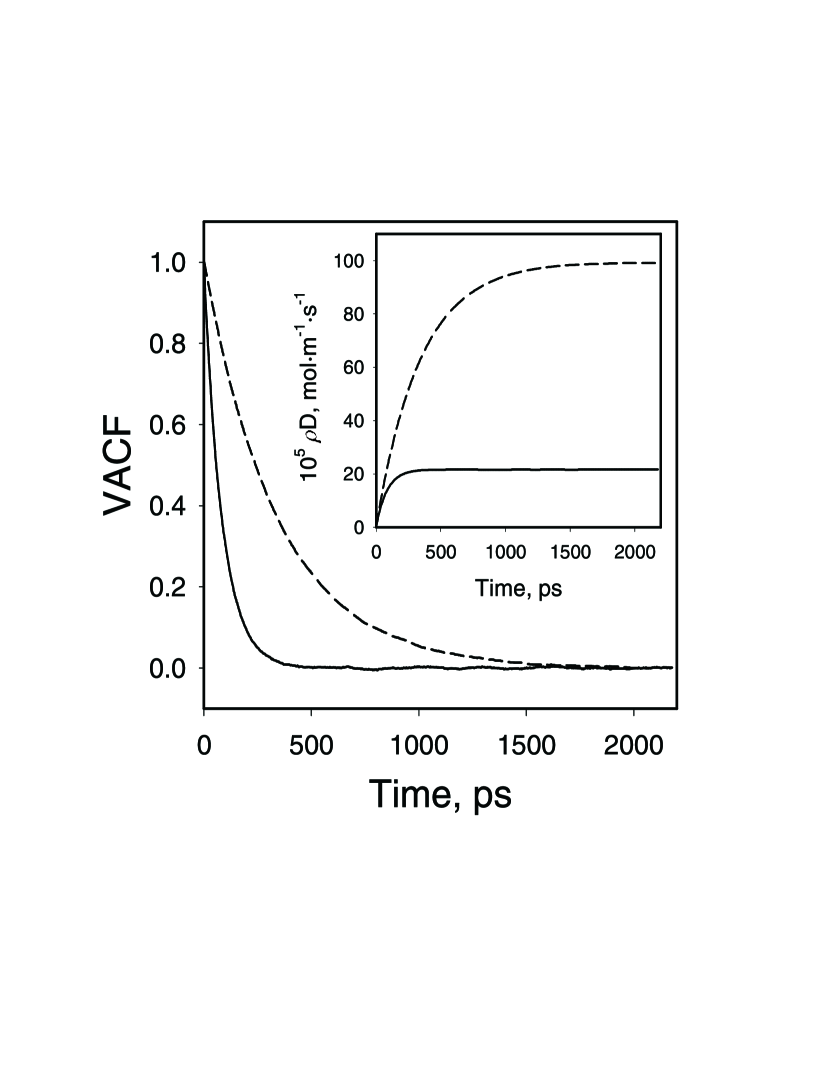
Figure 1:

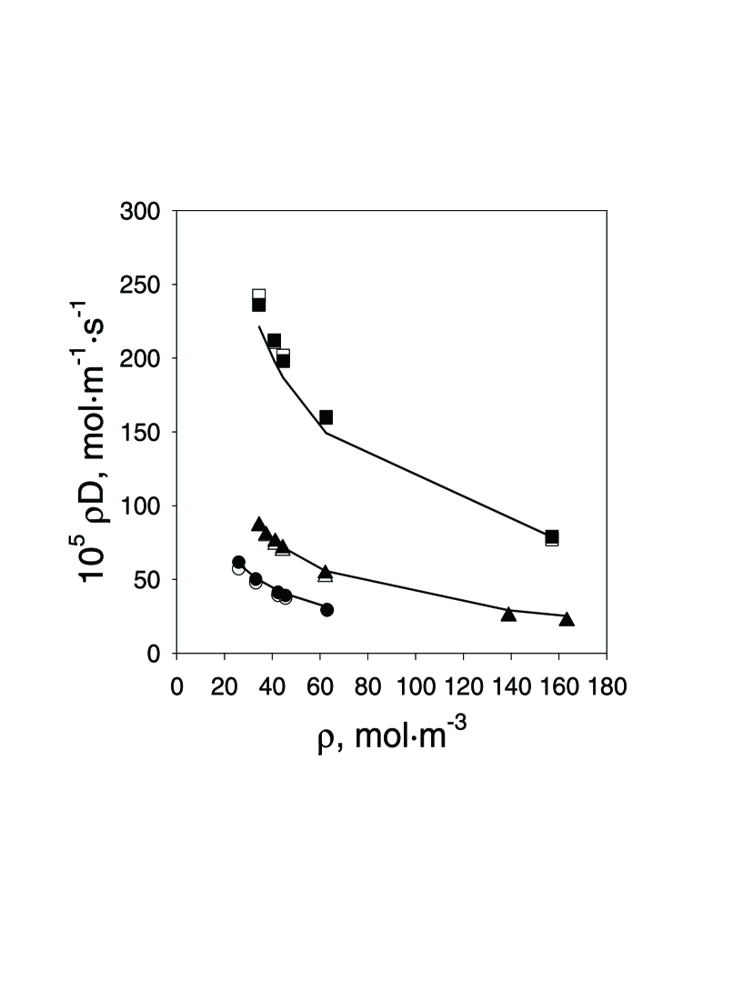
Figure 2:

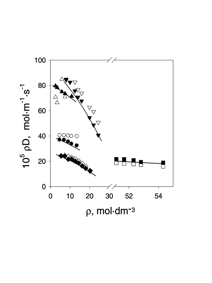
Figure 3:

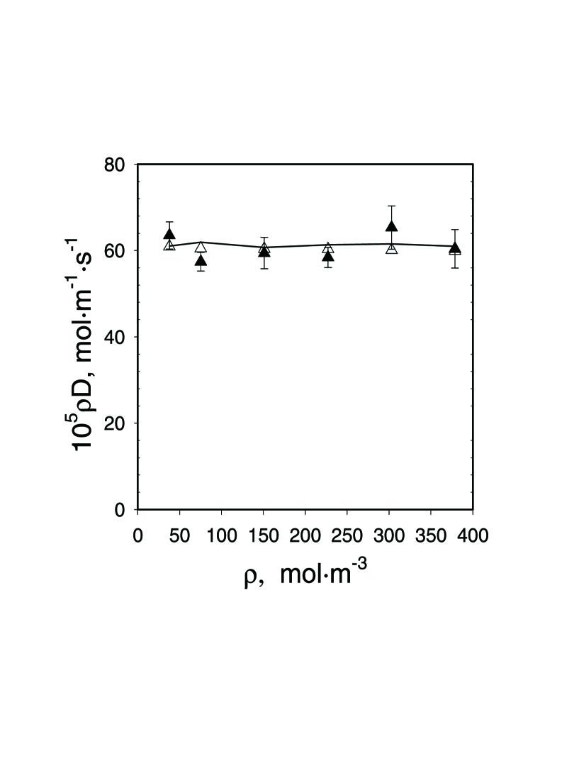
Figure 4:

Figure 5: