On modeling the scalar meson dynamics with Resonance Chiral Theory

Abstract:

The features of the Resonance Chiral Theory ($\rm{R}\chi{T}$) related to the description of the lightest scalar resonances, $\sigma$, $f_{0}(980)$ and $a_{0}(980)$, are discussed. Major attention is paid to the fits of the invariant mass distributions in the radiative decays of the $\phi(1020)$ meson ($\phi\to(\gamma a_{0}\to)\gamma\pi\eta$ and $\phi\to(\gamma f_{0}/\sigma\to)\gamma\pi\pi$). The study of the scalar sector in $\rm{R}\chi{T}$ is motivated by the success of the theory predictive power in numerous processes with other types of resonances. We conclude that $\rm{R}\chi{T}$ is sufficiently flexible to describe these decays, however the further quantitative improvement is required. The technical work-outs and related important questions are outlined.

1 Introduction

The Resonance Chiral Theory ($\rm{R}\chi{T}$) is a consistent extension of the Chiral Perturbation Theory (ChPT) to the region of energies near 1 GeV by explicit introduction of the resonance fields and exploiting the idea of resonance saturation [1]. One of the advantages of the $\rm{R}\chi{T}$ Lagrangian at leading order (LO) (which we essentially use in our approach) is that, having a good predictive power, it contains very few free parameters compared with the other phenomenological models.

The fields of $\rm{R}\chi{T}$, which correspond to meson resonances, are the large-$N_{c}$ narrow states with equal masses within the multiplet. The mass splitting corrections were worked-out in a consistent way for $J^{PC}=1^{--},2^{++},1^{++},1^{+-},0^{-+}$ nonets [2]. In the light scalar sector ($J^{PC}=0^{++}$) the deviation of mass matrix for physical states from its large-$N_{c}$ limit is large. There are also other indications that the $\mathcal{O}(1/N_{c})$ corrections are very important for the light scalar mesons. For the advances in the understanding the scalar mesons we refer to the corresponding section in the Particle Data Review [3] and the Proceedings of the recent Workshop dedicated to the subject [4].

There were numerous attempts to describe the dynamics of the lightest scalar mesons — $a_{0}(980)$ ($I^{G}=1^{-}$), $f_{0}(980)$ and $f_{0}(600)~{}\equiv~{}\sigma$ ($I^{G}=0^{+}$) — by means of chiral theories, e.g. [5, 6, 7]. In Ref. [5], for instance, a decade ago the light scalars were successfully united into the nonet and the subsequent symmetry relations were studied. The consideration of scalar sector in $\rm{R}\chi{T}$ usually avoided the explicit assignments for all of the multiplet members.

The technical work-outs from the $\rm{R}\chi{T}$ for the radiative decays with the scalar mesons can be found e.g.​ in Ref. [6]. The general features of the approach are sketched in Section 2. In Section 3 we pay attention to the important issues like removal of the scalar tadpole terms of the $\rm{R}\chi{T}$ Lagrangian and $\eta$ (and $\eta^{\prime}$) inclusion in $\rm{R}\chi{T}$.

The estimates of the model parameters in Ref. [6] were carried out in a naïve way (see [8]), however the interaction pattern and dynamic details remain solid and easily allow for the other ways of parameter extraction. Improvements on this way were initiated in Ref. [9] and this paper is aimed to this analysis as well. Section 4 is devoted to the fits of the invariant mass distributions in the radiative decays of the $\phi(1020)$ meson: $\phi\to(\gamma a_{0}\to)\gamma\pi\eta$ and $\phi\to(\gamma f_{0}/\sigma\to)\gamma\pi\pi$. For the extraction of the mixing parameter and the couplings we try to use the model-independent information on the pole position of $\sigma$ [10], pole position of $f_{0}(980)$ due to Ref. [11] and information on the $a_{0}(980)$ parameters from Ref. [12]. Brief conclusions are drawn in Section 5.

2 Scalar mesons in R$\chi$T

The scalar resonances below $1$ GeV ($\sigma$, $f_{0}(980)$ and $a_{0}(980)$) have important consequences for the low-energy hadronic interactions (e.g. they contribute to ChPT LECs in order $\mathcal{O}(p^{4})$). If one does not use any special (non-perturbative) techniques to account for corrections to the leading order in $1/N_{c}$, then to be consistent with the physics one has to introduce the resulting effects explicitly in the $\rm{R}\chi{T}$ Lagrangian. One may conclude that the large-$N_{c}$ counting has to be somewhat relaxed in favor of effects peculiar for the light scalars, at the same time the chiral symmetry has to be preserved. With the notation of Refs. [1, 2] the relevant Lagrangian reads

$$\mathcal{L}_{scalar} = \frac{1}{2}\langle\nabla^{\lambda}S\;\nabla_{\lambda}S-M_{S}^{2}\,S^{2}\rangle+e^{S}_{m}\left\langle S^{2}\;\chi_{+}\right\rangle+k^{S}_{m}S_{0}\left\langle S^{oct}\chi_{+}\right\rangle-\frac{\gamma^{S}_{m}\;M_{S}^{2}}{2}S_{0}^{2}+\mathcal{L}_{int},$$ (1)

$$\mathcal{L}_{int} = c_{d}\left\langle S\;u_{\mu}u^{\mu}\right\rangle+c_{m}\left\langle S\;\chi_{+}\right\rangle.$$ (2)

Scalar octet $S^{oct}$ and singlet $S_{0}$ fields are related to the physical degrees of freedom as follows:

$$\left\{\begin{aligned} a_{0}(980)=&S_{3},\\ f_{0}(980)=&S_{0}\,\cos\theta-S_{8}\,\sin\theta,\\ \sigma=&S_{0}\,\sin\theta+S_{8}\,\cos\theta.\end{aligned}\right.$$ (3)

Here $S_{3}$ is the isospin-one, $S_{8}$ is the isospin-zero neutral members of the flavor octet. There are indications for the $\sigma$, $f_{0}(980)$ and $a_{0}(980)$ mesons to be members of one multiplet [5, 13].

For the attempts to work out the mass splitting for lightest scalar mesons from the kinetic and mass part of Lagrangian (1) we refer to [2, 5]. In the current paper we assume that the values of $e^{S}_{m}$, $k^{S}_{m}$ and $\gamma^{S}_{m}$ are implicitly tuned in such a way, that the mass eigenvalues correspond to the observed poles. In principle, the mixing angle $\theta$ is determined by the mass diagonalization, however it also affects the interaction pattern of the physical states. Within the scope of the paper we fix the $\theta$ from fit to decay distributions.

In the interaction Lagrangian (2) the simplification $c_{m,d}S=c_{m,d}\left(S^{oct}+S_{0}/\sqrt{3}\right)$ is assumed. In notation of Ref. [1] it means that $\tilde{c}_{m,d}=c_{m,d}/\sqrt{3}$ in the large-$N_{c}$ limit. The coupling constants $c_{d}$ and $c_{m}$ have to be fixed from the measured decays. We use the $\phi$ radiative decay distributions for that purpose below in Section 4.

3 Scalar tadpoles, $\eta$ meson and pseudoscalar decay constants in $\rm{R}\chi{T}$

The pseudoscalar meson decay constant $F$ receives leading corrections at order $\mathcal{O}(p^{4})$ in ChPT due to the low energy constant $L_{5}$. The $\rm{R}\chi{T}$ framework at LO has effectively the same chiral order. It leads to the same corrections to the decay constants, when one removes the scalar tadpole term $\mathcal{L}^{tad}_{S}={2c_{m}}\left\langle S\chi\right\rangle$ and use the hypothesis of resonance saturation [14].

Let $\phi_{8}=\eta_{8}$ be the octet member, $\phi_{0}=\eta_{0}$ be the singlet state, and $\lambda_{0}\equiv\sqrt{2/3}\;{\rm diag}(1,1,1)$. Then the pseudoscalar nonet in $\rm{R}\chi{T}$ reads $u\equiv\exp\left(\frac{\rm i}{\sqrt{2}}\;\sum_{b=0}^{8}\frac{\lambda_{b}\phi_{b}}{\sqrt{2}f_{b}}\right)$, where $f_{b}$ had received corrections: $f_{1,2,3}\neq f_{4,5,6,7}\neq f_{8}\neq F$ due to $SU(3)$ flavor breaking and $f_{0}\neq f_{8}\neq F$ due to nonet symmetry breaking and topological effects of $U(1)$ axial anomaly. The singlet field also obtains an extra contribution to mass due to $U(1)$ axial anomaly. Translation of the $f_{b}$ constants into those for physical fields is done in the two-angle mixing scheme, for a review see [15],

$$\left(\begin{array}[]{cc}\langle 0|J_{\mu,\,5}^{8}(0)|\eta(p)\rangle&\langle 0|J_{\mu,\,5}^{0}(0)|\eta(p)\rangle\\ \langle 0|J_{\mu,\,5}^{8}(0)|\eta^{\prime}(p)\rangle&\langle 0|J_{\mu,\,5}^{0}(0)|\eta^{\prime}(p)\rangle\end{array}\right) = {\rm i}\sqrt{2}p_{\mu}\left(\begin{array}[]{lr}f_{8}\cos\theta_{8}&-f_{0}\sin\theta_{0}\\ f_{8}\sin\theta_{8}&f_{0}\cos\theta_{0}\end{array}\right)\equiv{\rm i}\sqrt{2}p_{\mu}\hat{f}.$$ (8)

For the pseudoscalar nonet in physical basis one gets

$$u = \exp\left(\frac{\rm i}{\sqrt{2}}\;\left[\frac{\vec{\pi}\vec{\sigma}}{\sqrt{2}f_{\pi}}+\frac{\lambda_{4}K_{4}+\lambda_{5}K_{5}+\lambda_{6}K_{6}+\lambda_{7}K_{7}}{\sqrt{2}f_{K}}+\frac{1}{\sqrt{2}}\;\left(\lambda_{8}\;\;\lambda_{0}\right)\!\hat{f}^{-1}\!\left(\begin{array}[]{l}\eta\\ \eta^{\prime}\end{array}\right)\right]\right)$$ (11)

$$\left\{\begin{array}[]{l}\eta_{8}=\frac{1}{\cos(\theta_{8}-\theta_{0})}\left[\eta\cos\theta_{0}+\eta^{\prime}\sin\theta_{0}\right]\\ \eta_{0}=\frac{1}{\cos(\theta_{8}-\theta_{0})}\left[-\eta\sin\theta_{8}+\eta^{\prime}\cos\theta_{8}\right],\end{array}\right.\;\;\;\;\;\;\left\{\begin{array}[]{l}\eta=\eta_{8}\cos\theta_{8}-\eta_{0}\sin\theta_{0}\\ \eta^{\prime}=\eta_{8}\sin\theta_{8}+\eta_{0}\cos\theta_{0}.\end{array}\right.$$ (16)

The mixing angles are determined [16, 17] from experiment. We use $\theta_{1}=-9.2^{\circ}\pm 1.7^{\circ}$ and $\theta_{8}=-21.2^{\circ}\pm 1.6^{\circ}$ [16], which correspond to $f_{8}=(1.26\pm 0.04)f_{\pi}$ and $f_{0}=(1.17\pm 0.03)f_{\pi}$.

In order to make the effective lagrangians read simpler one may apply the following notation

$$C_{q} \equiv\tfrac{f_{\pi}}{\sqrt{3}\cos(\theta_{8}-\theta_{0})}\left(\frac{1}{f_{0}}\cos\theta_{0}-\frac{1}{f_{8}}\sqrt{2}\sin\theta_{8}\right),\;\;\;\;\;\;\;\;C^{\prime}_{q} \equiv\tfrac{f_{\pi}}{\sqrt{3}\cos(\theta_{8}-\theta_{0})}\left(\tfrac{1}{f_{8}}\sqrt{2}\cos\theta_{8}+\tfrac{1}{f_{0}}\sin\theta_{0}\right),$$

$$C_{s} \equiv\tfrac{f_{\pi}}{\sqrt{3}\cos(\theta_{8}-\theta_{0})}\left(\frac{1}{f_{0}}\sqrt{2}\cos\theta_{0}+\tfrac{1}{f_{8}}\sin\theta_{8}\right),\;\;\;\;\;\;\;\;C^{\prime}_{s} \equiv\tfrac{f_{\pi}}{\sqrt{3}\cos(\theta_{8}-\theta_{0})}\left(\tfrac{1}{f_{8}}\cos\theta_{8}-\tfrac{1}{f_{0}}\sqrt{2}\sin\theta_{0}\right).$$

Then the pseudoscalar nonet can be written as

$$u \!\!\!\!= \!\!\!\!\exp\left(\frac{\rm i}{\sqrt{2}f_{\pi}}\left(\begin{array}[]{ccc}\frac{\pi^{0}+C_{q}\eta+C_{q}^{\prime}\eta^{\prime}}{\sqrt{2}}&\pi^{+}&\frac{f_{\pi}}{f_{K}}{K^{+}}\\ \pi^{-}&\frac{-\pi^{0}+C_{q}\eta+C_{q}^{\prime}\eta^{\prime}}{\sqrt{2}}&\frac{f_{\pi}}{f_{K}}{K^{0}}\\ \frac{f_{\pi}}{f_{K}}{K^{-}}&\frac{f_{\pi}}{f_{K}}{\bar{K}^{0}}&-C_{s}\eta+C_{s}^{\prime}\eta^{\prime}\end{array}\right)\right).$$ (20)

4 The $\phi(1020)$ radiative decay fits

The dominant decay channels of the scalar mesons are known to be $\pi^{+}\pi^{-}$, $\pi^{0}\pi^{0}$ for $f_{0}(980)$ and $\sigma$ meson, and $\pi^{0}\eta$ for $a_{0}(980)$ meson. Much experimental attention has been paid so far to the radiative decay of the $\phi$ meson: $\phi(1020)\to\gamma a_{0}\to\gamma\pi\eta$ [18, 19] and $\phi(1020)\to\gamma f_{0}\to\gamma\pi\pi$ [20]. Various models (e.g. [6, 7]) have been proposed to describe these decays. In our previous consideration [9] we performed the separate fits ($\pi^{0}\pi^{0}$ and $\pi\eta$) for the mass-parameters of scalar mesons and the angle $\theta$, while $4c_{d}c_{m}=F^{2}$ and $c_{d}=c_{m}$ relations of Ref. [21] were imposed. The $\sigma$ meson contribution was not taken into account and the data points with $m_{\pi\pi}>700$ MeV were fitted. We ended up with $\chi^{2}/{dof}=2.05\,(\pi^{0}\pi^{0})$, and $\chi^{2}/{dof}=3.32\,(\pi\eta)$ in a fit to combined KLOE and Novosibirsk data.

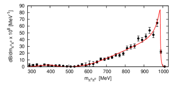
Figure 1: “Best fit”: $\chi^{2}/d.o.f.(tot)=1.47$, $c_{d}=93^{+11}_{-5}$, $c_{m}=46^{+9}_{-2}$, $M_{a_{0}}=1150^{+50}_{-23}$, $M_{f_{0}}=986.1^{+0.4}_{-0.5}$, $M_{\sigma}=504^{+242}_{-53}$, $\theta=36^{o}\pm 2^{o}$ (errors from MINOS only). Data:  [19, 20].

Let $\tilde{M}_{S}={M}_{S}-i/2\;\Gamma$ be the complex pole of the amplitude. We define the scalar meson propagator (see discussion e.g. in [22]) as

$$D_{S}^{-1}(p^{2}) = p^{2}-\Re\mathrm{e}\left(\tilde{M}_{S}^{2}+i\,\tilde{M}_{S}\;\tilde{\Gamma}_{S,\;{tot}}(\tilde{M}_{S}^{2})\right)+i\,\sqrt{p^{2}}\;\tilde{\Gamma}_{S,\;{tot}}(p^{2}),$$ (21)

with the Flatté-modified [23] widths

$$\tilde{\Gamma}_{f_{0},\;\sigma,\,tot}(p^{2}) = \tilde{\Gamma}_{f_{0},\;\sigma\to\pi\pi}(p^{2})+\tilde{\Gamma}_{f_{0},\;\sigma\to K\bar{K}}(p^{2}),$$ (22)

$$\tilde{\Gamma}_{a_{0},\,tot}(p^{2}) = \tilde{\Gamma}_{a_{0}\to\pi^{0}\eta}(p^{2})+\tilde{\Gamma}_{a_{0}\to K\bar{K}}(p^{2}).$$

These analytic functions of (complex) $p^{2}$ (continued below the thresholds through $\sqrt{{p^{2}}/{4}-m^{2}}=i\sqrt{|{p^{2}}/{4}-m^{2}|}$) are given in Appendix A. One should notice that the exact propagator is of course different from (21). Thus the proper positions of the amplitude poles, $\tilde{M}_{S}$, do not coincide with the zeros of $D^{-1}(p^{2})$ defined by (21), in other words, $D^{-1}(\tilde{M}_{S}^{2})\neq 0$. Nevertheless, it is of interest to investigate how the form (21) reproduces the data. We use the information on the poles from [10, 11, 12] and perform the following fits to the $\phi(1020)$ radiative decay spectra of Refs. [19, 20]:

• fixed: $c_{d}=c_{m}=F/2\approx 46.2$ MeV [21]; (cf. Ref. [9])
  fitted (A): $M_{a_{0}}$ to $\pi\eta$ spectrum, $M_{f_{0}}$, $\theta$ to $\pi^{0}\pi^{0}$ spectrum, $m_{\pi\pi}>700$ MeV (separate fits);
  fitted (B): $M_{a_{0}}$ to $\pi\eta$ spectrum, $M_{f_{0}}$, $M_{\sigma}$, $\theta$ to $\pi^{0}\pi^{0}$ spectrum (separate fits);

• fixed (C, D): $\tilde{M}_{a_{0}}=(985\pm 10)-i\;(50\pm 17)$ [12], $\tilde{M}_{f_{0}}=1001-i\;16$ [11];
  fixed (E): $\tilde{M}_{a_{0}}$ [12], $\tilde{M}_{f_{0}}$ [11], $\tilde{M}_{\sigma}=441^{+16}_{-8}-i\;272^{+9}_{-13}$ [10]
  fitted: $c_{d}$, $c_{m}$, $\theta$ to $\pi\eta$ and $\pi^{0}\pi^{0}$ spectra (simultaneous fit); $m_{\pi\pi}>700$ MeV in C;

• fitted: $M_{a_{0}}$, $M_{f_{0}}$, (and $M_{\sigma}$ in F), $c_{d}$, $c_{m}$, $\theta$ to $\pi\eta$ and $\pi^{0}\pi^{0}$ spectra (simultaneous fit).

For $\phi(1020)\to\gamma a_{0}\to\gamma\pi\eta$ we use only $\eta\to\gamma\gamma$ data sample of Ref. [18] and exclude the two rightmost points from fit. The results are shown in Table 1. The best fit including $\sigma$ meson is Fit F, it is illustrated in Fig. 1. For Fits C, D, E we employed (21), while for Fits A, B and F we assumed $\tilde{M}_{s}\approx M_{s}$ in (21) and employed

$$D_{S}^{-1}(p^{2}) = p^{2}-M_{S}^{2}+M_{S}\;\Im\!\mathrm{m}\!\left(\tilde{\Gamma}_{S,\;{tot}}(M_{S}^{2})\right)+i\,\sqrt{p^{2}}\;\tilde{\Gamma}_{S,\;{tot}}(p^{2}).$$ (23)

Table 1: MINUIT fit results. Shown errors are due to MINOS. The fixed input values are marked by asterisk. Couplings and masses are given in MeV.

							$\chi^{2}/{dof}$
Fit	$c_{d}$	$c_{m}$	$M_{a_{0}}$	$M_{f_{0}}$	$M_{\sigma}$	$\theta$	$\pi\pi$	$\pi\eta$	$tot.$
A	$46.2^{\ast}$	$46.2^{\ast}$	$1030\pm 7$	$979.8^{+0.9}_{-0.9}$	—	$21^{o}\pm 1^{o}$	$2.95$	$4.73$	—
B	$46.2^{\ast}$	$46.2^{\ast}$	$1030\pm 7$	$979.0^{+0.8}_{-0.8}$	$441^{+15}_{-25}$	$21^{o}\pm 1^{o}$	$2.78$	$4.73$	—
C	$68\pm 4$	$27\pm 3$	$985^{\ast}$	$1001^{\ast}$	—	$22^{o}\pm 2^{o}$	$14.25$	$12.93$	$12.7$
D	$131^{+14}_{-12}$	$73^{+7}_{-5}$	$985^{\ast}$	$1001^{\ast}$	—	$23^{o}\pm 1^{o}$	$6.25$	$2.48$	$5.15$
E	$158^{+12}_{-12}$	$67^{+4}_{-5}$	$985^{\ast}$	$1001^{\ast}$	$441^{\ast}$	$30^{o}\pm 1^{o}$	$4.12$	$3.30$	$3.77$
F	$93^{+11}_{-5}$	$46^{+9}_{-2}$	$1150^{+50}_{-23}$	$986.1^{+0.4}_{-0.5}$	$504^{+242}_{-53}$	$36^{o}\pm 2^{o}$	$1.32$	$2.07$	$1.47$

5 Conclusions

The current results are the good illustration of the model machinery. There are important theoretical issues in the scalar sector of $\rm{R}\chi{T}$. Scalar tadpoles and their relevance for the corrections to pseudoscalar meson decay constants and problem of consistent mass splitting for resonances are among them. It was also not widely known that the account for the $\eta-\eta^{\prime}$ mixing at leading order in $\rm{R}\chi{T}$ requires the two-angle scheme in the singlet-octet basis.

We have performed several fits to the $\phi(1020)$ radiative decay spectra [19, 20] in order to fix the $\rm{R}\chi{T}$ parameters in the scalar sector. It is observed, that the quality of the fit strongly depends on the form used for the scalar propagator. We used the information on the pole positions in order to pin down the masses of scalars in the fit and concluded that this way seems problematic within the currently used Flatté-like framework. Our best result is the combined Fit F, in which $\sigma$ meson contribution is accounted for. It covers the full range of the invariant masses and has total $\chi^{2}/d.o.f.=1.47$.

Appropriate and numerically optimal way to fix the model parameters is still to be developed. The above consideration gives a strong motivation for the further improvement of the model.

Appendix A Model details for the scalar meson propagators

Here we list the reference formulae (see also [9]). The momentum-dependent widths read

$$\tilde{\Gamma}_{f_{0},\sigma\to\pi\pi,KK}(p^{2}) = \frac{3}{2}\frac{1}{2p^{2}}\sqrt{\frac{p^{2}}{4}-m_{\pi,K}^{2}}\;{\frac{G_{f_{0},\sigma\pi\pi,KK}^{2}(p^{2})}{4\pi}},$$ (24)

$$\tilde{\Gamma}_{a_{0}\to\pi\eta}(p^{2}) = \frac{1}{2p^{2}}\sqrt{\frac{(p^{2}+m_{\pi}^{2}-m_{\eta}^{2})^{2}}{4p^{2}}-m_{\pi}^{2}}\;\frac{G_{a_{0}\pi\eta}^{2}(p^{2})}{4\pi},$$

$$\tilde{\Gamma}_{a_{0}\to K\bar{K}}(p^{2}) = 2\,\frac{1}{2p^{2}}\sqrt{\frac{p^{2}}{4}-m_{K}^{2}}\;{\frac{G_{a_{0}KK}^{2}(p^{2})}{4\pi}}.$$

It is assumed that $\sqrt{f(p^{2})}=e^{i\;Arg(f(p^{2}))/2}\sqrt{|f(p^{2})|}$ if necessary (below the two-kaon threshold). In the $\rm{R}\chi{T}$ formalism the effective couplings for the scalars are momentum-dependent:

$$G_{f_{0},\;\sigma KK}(p^{2}) \equiv 1/f_{K}^{2}\;\left(\hat{g}_{f_{0},\;\sigma KK}(m_{K}^{2}-p^{2}/2)+g_{f_{0},\;\sigma KK}\right),$$ (25)

$$G_{f_{0},\;\sigma\pi\pi}(p^{2}) \equiv 1/f_{\pi}^{2}\;\left(\hat{g}_{f_{0},\;\sigma\pi\pi}(m_{\pi}^{2}-p^{2}/2)+g_{f_{0},\;\sigma\pi\pi}\right),$$

$$G_{a_{0}KK}(p^{2}) \equiv 1/f_{K}^{2}\;\left(\hat{g}_{a_{0}KK}(m_{K}^{2}-p^{2}/2)+g_{a_{0}KK}\right),$$

$$G_{a_{0}\pi\eta}(p^{2}) \equiv 1/f_{\pi}^{2}\;\left(\hat{g}_{a\pi\eta}(m_{\eta}^{2}+m_{\pi}^{2}-p^{2})/2+g_{a\pi\eta}\right).$$

The Lagrangian parameters enter these formulae via

$$g_{aKK} = -\sqrt{2}\,c_{m}m_{K}^{2},$$

$$g_{a\pi\eta} = -2\sqrt{2}\,C_{q}\,c_{m}\,m_{\pi}^{2},$$

$$\hat{g}_{aKK} = \sqrt{2}\,c_{d},$$

$$\hat{g}_{a\pi\eta} = 2\sqrt{2}\,C_{q}\,c_{d}$$

$$g_{f\pi\pi} = -2\,c_{m}\,m_{\pi}^{2}(2\,\cos\theta-\sqrt{2}\,\sin\theta)/\sqrt{3},$$

$$g_{fKK} = -c_{m}\,m_{K}^{2}(4\,\cos\theta+\sqrt{2}\,\sin\theta)/\sqrt{3},$$

$$\hat{g}_{f\pi\pi} = 2\,c_{d}(2\cos\theta-\sqrt{2}\,\sin\theta)/\sqrt{3},$$

$$\hat{g}_{fKK} = c_{d}(4\cos\theta+\sqrt{2}\sin\theta)/\sqrt{3},$$

$$g_{{\sigma}\pi\pi} = -2\,c_{m}\,m_{\pi}^{2}(\sqrt{2}\,\cos\theta+2\,\sin\theta)/\sqrt{3},$$

$$g_{{\sigma}KK} = -c_{m}\,m_{K}^{2}(-\sqrt{2}\,\cos\theta+4\,\sin\theta)/\sqrt{3},$$

$$\hat{g}_{{\sigma}\pi\pi} = 2\,c_{d}(\sqrt{2}\cos\theta+2\,\sin\theta)/\sqrt{3},$$

$$\hat{g}_{{\sigma}KK} = c_{d}(-\sqrt{2}\,\cos\theta+4\,\sin\theta)/\sqrt{3}.$$

References

- [1] G. Ecker, J. Gasser, A. Pich, E. de Rafael, The role of resonances in chiral perturbation theory, Nucl. Phys. B 321 (1989) 311.
- [2] V. Cirigliano, G. Ecker, H. Neufeld and A. Pich, Meson resonances, large- and chiral symmetry, JHEP 0306 (2003) 012 [hep-ph/0305311].
- [3] C. Amsler et al., The Review of Particle Physics, Phys. Lett. B 667 (2008) 1.
- [4] Proceedings of SCADRON70: Workshop on Scalar Mesons and Related Topics Honoring Michael Scadron’s 70th Birthday, ed. G. Rupp et al., AIP Conf. Proc. 1030 (2008); ISBN 978-7354-0554-7.
- [5] D. Black, A. H. Fariborz, F. Sannino and J. Schechter, Putative Light Scalar Nonet, Phys. Rev. D 59 (1999) 074026 [hep-ph/9808415].
- [6] S. Ivashyn and A. Y. Korchin, Radiative decays with light scalar mesons and singlet-octet mixing in ChPT, Eur. Phys. J. C 54 (2008) 89 [0707.2700 [hep-ph]].
- [7] D. Black, M. Harada, J. Schechter, Chiral approach to phi radiative decays, Phys. Rev. D 73 (2006) 054017.
- [8] S. Ivashyn and A. Korchin, Radiative decays with and from ChPT at order , AIP Conf. Proc. 1030 (2008) 123 [0805.4088 [hep-ph]].
- [9] S. Ivashyn and A. Korchin, Radiative decays with scalar mesons a0(980) and f0(980) in Resonance Chiral Theory, Nucl. Phys. Proc. Suppl. 181-182 (2008) 189 [0901.4045 [hep-ph]].
- [10] I. Caprini, G. Colangelo and H. Leutwyler, Mass and width of the lowest resonance in QCD, Phys. Rev. Lett. 96 (2006) 132001.
- [11] M.R. Pennington et al., Amplitude analysis of high statistics results on and the two photon width of isoscalar states, Eur. Phys. J. C 56 (2008) 1.
- [12] L3 Collaboration, P. Achard et al., formation in in two-photon collisions at LEP, Phys. Lett. B 526 (2002) 269.
- [13] J. A. Oller, The mixing angle of the lightest scalar nonet, Nucl. Phys. A 727 (2003) 353.
- [14] J. J. Sanz Cillero, Pion and kaon decay constants: Lattice versus resonance chiral theory, Phys. Rev. D 70 (2004) 094033 [hep-ph/0408080].
- [15] T. Feldmann, Quark structure of pseudoscalar mesons, Int. J. Mod. Phys. A 15 (2000) 159.
- [16] T. Feldmann, P. Kroll, B. Stech, Mixing and decay constants of pseudoscalar mesons, Phys. Rev. D 58 (1998) 114006 [hep-ph/9802409].
- [17] R. Escribano and J. M. Frere, Study of the system in the two mixing angle scheme, JHEP 0506 (2005) 029 [hep-ph/0501072].
- [18] KLOE Collaboration, A. Aloisio et al., Study of the decay with the KLOE detector, Phys. Lett. B 536 (2002) 209 [hep-ex/0204012].
- [19] KLOE Collaboration, C. Bini et al., Fit to the invariant mass spectra of the decays and , KLOE Note 173 (2002).
- [20] KLOE Collaboration, A. Aloisio et al., Study of the decay with the KLOE detector, Phys. Lett. B 537 (2002) 21 [hep-ex/0204013].
- [21] M. Jamin, J. A. Oller and A. Pich, Strangeness-changing scalar form factors, Nucl. Phys. B 622 (2002) 279 [hep-ph/0110193].
- [22] R. Escribano, A. Gallegos, J. L. Lucio M, G. Moreno and J. Pestieau, On the mass, width and coupling constants of the f0(980), Eur. Phys. J. C 28 (2003) 107 [arXiv:hep-ph/0204338].
- [23] S.M. Flatté, Coupled - Channel Analysis Of The Pi Eta And K Anti-K Systems Near K Anti-K Threshold, Phys. Lett. B 63 (1976) 224.