Forward and inverse cascades in decaying two-dimensional electron magnetohydrodynamic turbulence

Abstract

Electron magnetohydrodynamic (EMHD) turbulence in two dimensions is studied via high-resolution numerical simulations with a normal diffusivity. The resulting energy spectra asymptotically approach a $k^{-5/2}$ law with increasing $R_{B}$, the ratio of the nonlinear to linear timescales in the governing equation. No evidence is found of a dissipative cutoff, consistent with non-local spectral energy transfer. Dissipative cutoffs found in previous studies are explained as artificial effects of hyperdiffusivity. Relatively stationary structures are found to develop in time, rather than the variability found in ordinary or MHD turbulence. Further, EMHD turbulence displays scale-dependent anisotropy with reduced energy transfer in the direction parallel to the uniform background field, consistent with previous studies. Finally, the governing equation is found to yield an inverse cascade, at least partially transferring magnetic energy from small to large scales.

Copyright 2009 American Institute of Physics. This article may be downloaded for personal use only. Any other use requires prior permission of the author and of the American Institute of Physics.

The following article appearing in Physics of Plasmas, 16, 042307 (2009) and may be found at (http://link.aip.org/link/?PHP/16/042307).

I Introduction

Turbulence plays a crucial role in a wide variety of geophysical and astrophysical fluid flows. In this paper we present results on a particular type of plasma turbulence in which the flow is entirely due to the electrons, with the ions forming a static background. The equation governing the electrons’ self-induced magnetic field is then

$$\frac{\partial{\bf B}}{\partial t}=-\nabla\times\left[{\bf J}\times{\bf B}\right]+R_{B}^{-1}\ \nabla^{2}{\bf B},$$ (1)

where ${\bf J}=\nabla\times{\bf B}$, and $R_{B}={\sigma B_{0}}/{nec}$, with $\sigma$ the conductivity, $B_{0}$ a measure of the field strength, $n$ the electron number density, $e$ the electron charge, and $c$ the speed of light. See for example Goldreich & Reisenegger (1992), who derived this equation in the context of magnetic fields in the crusts of neutron stars. More generally though, it is applicable in many weakly collisional, strongly magnetic plasmas, so other applications could include the Sun’s corona or the Earth’s magnetosphere.

Turbulence governed by (1) is known as electron MHD (EMHD), Hall MHD, or whistler turbulence. Based on its (at least superficial) similarity to the vorticity equation governing ordinary, nonmagnetic turbulence,

$$\frac{\partial{\bf w}}{\partial t}=\nabla\times\left[{\bf u}\times{\bf w}\right]+Re^{-1}\ \nabla^{2}{\bf w},$$ (2)

where now ${\bf w}=\nabla\times{\bf u}$, Goldreich & Reisenegger (1992) argued that (1) would initiate a turbulent cascade to small lengthscales, thereby accelerating neutron stars’ magnetic field decay beyond what ohmic decay acting on large lengthscales could achieve. They suggested in particular that the turbulent spectrum would scale as $k^{-2}$, with a dissipative cutoff occurring at $k\sim R_{B}$.

However, there are also some quite fundamental differences between equations (1) and (2). In (2) the dissipative term contains more derivatives than the nonlinear term, so on sufficiently short lengthscales the dissipative term will always dominate. In contrast, in (1) the two terms both contain two derivatives, so it is conceivable that the nonlinear term will always dominate, even on arbitrarily short lengthscales. As pointed out by Hollerbach & Rudiger (2002), one obtains a dissipative cutoff only if one assumes that the cascade is local in Fourier space, coupling wavenumbers only to their immediate neighbors.

Indeed, whether the coupling is local or not is another important difference between (1) and (2). In (2) it is at least predominantly local; for example, very small scale structures see the largest structures as an essentially uniform background flow that simply advects them along, but without altering the nature of the small scale turbulence. In contrast, in (1) there is no such translational invariance; adding even an exactly uniform background field alters the dynamics of the small scale structures (as we will show in detail below). Similarly, in classical MHD turbulence, adding a background flow has no essential effect, but adding a background field does.

In this paper we present high-resolution numerical simulations of (1) in a two-dimensional periodic box geometry, designed specifically to address such questions as whether there is a dissipative cutoff or not, and whether the coupling is local or not. In contrast to previous simulations Biskamp, Schwarz & Drake (1996); Biskamp et al. (1999); Dastgeer et al. (2000); Dastgeer & Zank (2003); Cho & Lazarian (2004); Shaikh & Zank (2005), we do not employ hyperdiffusivity, which would of course disrupt this feature that the two terms in (1) have the same number of derivatives, and hence introduce an artificial dissipative cutoff. We also consider the question of whether (1) is capable of yielding an inverse cascade, and find that magnetic energy can be at least partially transferred from small to large scales.

II Equations

For two-dimensional fields, we may decompose $\bf B$ as

$${\bf B}={\bf B}_{p}+{\bf B}_{t}=\nabla\times(a\hat{{\bf e}}_{z})+b\hat{{\bf e}}_{z}.$$ (3)

where $a$ and $b$ depend only on $x$, $y$, $t$, but not $z$. Equation (1) then yields

$$\frac{\partial a}{\partial t}=R_{B}^{-1}\nabla^{2}a-(a_{y}b_{x}-a_{x}b_{y}),$$ (4)

and

$$\frac{\partial b}{\partial t}=R_{B}^{-1}\nabla^{2}b+(a_{y}\nabla^{2}a_{x}-a_{x}\nabla^{2}a_{y}),$$ (5)

where subscripts indicate derivatives.

Continuing our comparison of equations (1) and (2), it is instructive to note also that in (2) we would only have ${\bf u}={\bf u}_{p}=\nabla\times(\Psi\hat{{\bf e}}_{z})$, yielding

$$\frac{\partial\nabla^{2}\Psi}{\partial t}=Re^{-1}\nabla^{4}\Psi-[\Psi_{y}\ (\nabla^{2}\Psi)_{x}-\Psi_{x}\ (\nabla^{2}\Psi)_{y}].$$ (6)

Any additional ${\bf u}_{t}=v\hat{{\bf e}}_{z}$ would simply be advected by $\Psi$ as a passive scalar, but without any influence back on $\Psi$. This difference between (4) and (5) on the one hand, and (6) on the other merely reflects once again some of the differences between (1) and (2), in this case the lack of translational invariance in (1).

We solve (4) and (5) by expanding $a$ and $b$ in Fourier series in $x$ and $y$, and using standard pseudospectral techniques for the evaluation of the nonlinear terms, with dealiasing according to the 2/3 rule. The code employs the FFTW library Frigo & Johnson (2005) to achieve massive parallelisation on a suitable supercomputer. The time integration is done using a second order Runge-Kutta method. We performed a variety of runs, typically employing 64 processors, with the highest extending to $k=682$ in Fourier space, corresponding to $N=2048$ collocation points in real configuration space. Because of the two derivatives in the nonlinear term, the required timesteps are unfortunately very small, roughly proportional to $1/(N^{2})$. Values as small as $\sim 3\times 10^{-8}$ were used, requiring $O(10^{7})$ timesteps in total to reach $t=0.2$.

II.1 Initial Conditions

Since we are interested in freely decaying rather than forced turbulence, we need to carefully consider the nature of our chosen initial conditions. We will present results for three different sets of runs.

First, to study homogeneous forward cascades, we start off with random $O(1)$ energies in all Fourier modes up to $k=\sqrt{k_{x}^{2}+k_{y}^{2}}=5$, making sure that the poloidal $a$ and toroidal $b$ components have comparable amounts of energy. After initialisation the overall amplitude of the field is rescaled to ensure that the rms value of $|{\bf B}|=1$ at $t=0$.

Second, to study nonhomogeneous forward cascades, we start off with the same initialisation as above, but now add a uniform field $C\hat{\bf e}_{x}$, where $C=1$, 2 or 4. Note though that such a uniform field cannot be represented by an expansion of the form (3), at least not if $a$ and $b$ are to be periodic in $x$ and $y$. Instead, this field is simply added in to (3) directly, resulting in suitably modified equations (4) and (5).

Third, to explore the possibility of inverse cascades, we return to the $C=0$ case without any large scale magnetic field and now inject energy into modes in the range $10\leq k\leq 20$. The question then is how much of this initial energy moves to $k<10$, and how much moves to $k>20$.

Finally, for all three sets of results, each individual run was repeated with a number of different random initial conditions, to ensure that the results presented here are indeed representative.

II.2 Ideal Invariants

Equations (4) and (5) also have some useful associated diagnostics, corresponding to quantities that are conserved in the ideal, $R_{B}^{-1}\to 0$, limit. Specifically, we have equations for the energy and the magnetic helicity,

$$\frac{d}{dt}{\frac{1}{2}\int{\bf B}^{2}\,{\rm d}V}=-R_{B}^{-1}\int{\bf J}^{2}\,{\rm d}V,$$ (7)

$$\frac{d}{dt}{\frac{1}{2}\int{\bf A\cdot B}\,{\rm d}V}=-R_{B}^{-1}\int{\bf B\cdot J}\,{\rm d}V,$$ (8)

where $A$ is the vector potential, defined by ${\bf B=\nabla\times A}$. Note though that in the presence of a uniform background field, helicity is not even defined Berger (1997), let alone conserved.

These two equations are valid in both 2 and 3 dimensions. In 2 dimensions only, we have the additional quantity of the mean squared magnetic potential, known as anastrophy

$$\frac{d}{dt}{\frac{1}{2}\int a^{2}\,{\rm d}V}=-R_{B}^{-1}\int(a_{x}^{2}+a_{y}^{2})\,{\rm d}V,$$ (9)

which is in some ways perhaps analogous to enstrophy, which is also defined only for (6) in 2D, but not for (2) in 3D. However, anastrophy is not the same as enstrophy, and there does not appear to be any reason why conservation of anastrophy would necessarily imply an inverse cascade in the way that conservation of enstrophy forces inverse cascades to exist in 2D hydrodynamic turbulence.

In addition to the physical insight that they yield into the nature of the Hall nonlinearity, these various integrated quantities also offer useful diagnostic checks of the code. Reassuringly, we found that all of them (except helicity in a uniform field of course) were satisfied to within 0.1% or better by all of our runs.

III Results

III.1 Large-scale initial conditions

The energy spectrum, $E_{k}$, of 3D hydrodynamic turbulence is characterised by $E_{k}\propto k^{-5/3}$, the familiar Kolmogorov law Kolmogorov (1941). In 2D, the conservation of enstrophy forces an inverse cascade which leads to a much steeper spectrum $E_{k}\propto k^{-\alpha}$ with $\alpha>3$. In the case of 2D MHD turbulence, the spectral energy transfer rate is reduced which leads to a flatter energy spectrum $E_{k}\propto k^{-3/2}$, the Iroshnikov-Kraichnan spectrum Kraichnan & Montgomery (1980). Recent studies of EMHD turbulence have found, via methods which all employ hyperdiffusivity, a 5/3 Kolmogorov spectrum for small scales $kd_{e}>1$, equivalent to $k>O(R_{B})$, and a steeper 7/3 spectrum for longer wavelengths Biskamp, Schwarz & Drake (1996); Biskamp et al. (1999); Dastgeer et al. (2000); Dastgeer & Zank (2003); Cho & Lazarian (2004).

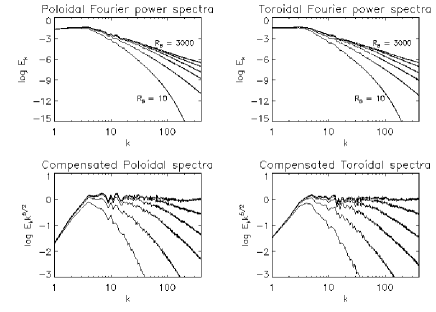
Figure 1: Energy spectra of homogeneous 2D EMHD turbulence at $t=0.2$. Across the top row are shown spectra for both toroidal and poloidal fields for $R_{B}=10$, 30, 100, 300, 1000 & 3000. Across the bottom row are compensated energy spectra $k^{5/2}E_{k}$.

In the upper plot of Figure 1, we show the poloidal and toroidal energy spectra of our solutions for $R_{B}=10$, 30, 100, 300, 1000 & 3000, evolved to a time $t=0.2$. The energy spectra have been stationary since approximately $t=0.12$ and time averaging between 0.12 and 0.2 reveals an identical spectrum and no further information. We interpret this to mean our simulations are resolved and evolved to a suitable time for inspection of the quasi-stationary cascade.

Both poloidal and toroidal energy spectra start out much the same at low $k$ and then lower $R_{B}$ spectra smoothly drop off with increasing $k$ whilst higher $R_{B}$ spectra maintain a linear gradient in the log-log plot. Transfer of energy to higher $k$ is then more efficient at higher $k$. The spectra are asymptotically approaching an energy spectrum $E_{k}\propto k^{-\nu}$, where $\nu=2.5\pm 0.1$. In the lower plot of Figure 1, we show compensated energy spectra to show this approach to $k^{-5/2}E_{k}=1$ with increasing $R_{B}$. Our value of $\nu$ is not compatible with $-2$ predicted by Goldreich & Reisenegger (1992) for 3D EMHD turbulence. Their prediction was calculated using a phenomenology based on Kraichnan’s arguments (the whistler effect) which has been shown by Dastgeer et al. (2000) to have little effect on the energy spectrum of 2D EMHD, rather it is thought to influence the subtle properties of the cascade like anisotropy which we discuss further in the next section. The spectral index we find is much more compatible with $\nu=7/3$ found by Biskamp et al. (1999) via numerical simulation for the $kd_{e}>1$ regime.

None of the spectra show any sign of a dissipative cutoff. By definition, the dissipation scale should occur when the local value of $R_{B}$ is $O(1)$ in equation 1. It is unclear though when this occurs since the definition of $R_{B}$ does not involve length scales. If the coupling is purely local in wavenumber, then this definition does involve length scales after all, since the $B_{0}$ that should be used is the field at that wavenumber only, rather than the total field. That is, according to the definition of Hollerbach & Rudiger (2002) where this argument was first developed, we have

$$R_{B}^{\prime}=R_{B}(B^{\prime}/B)$$ (10)

where the primed quantities are the small-scale local values and the unprimed the large-scale global. If we now suppose a $k^{-5/2}$ energy spectrum, then $B^{\prime}/B\sim k^{-5/4}$ and so $R_{B}^{\prime}$ is reduced to $O(1)$ when $k\sim R_{B}^{4/5}$. So, at $R_{B}=1000$ we would see a dissipative cutoff at $k\sim 250$. We do not see a dissipative cutoff at this scale. We can reconcile this by realising that this argument crucially depends on the coupling being local in Fourier space: if this does not hold then $R_{B}^{\prime}=R_{B}$ and there is simply no definite dissipation scale, as we find here.

We conclude therefore that the nonlinear term is able to dominate at all length scales and the coupling is non-local in Fourier space. This is not entirely unexpected, since both the terms in (1) contain two derivatives, but it is in contrast to previous studies. It should be emphasized that other authors have been unable to properly address the question of a dissipative cutoff since hyperdiffusivity has masked the effect of the nonlinear term at high $k$. This may also explain the discrepancy between the spectral index of 5/2 we find and previous values of 7/3.

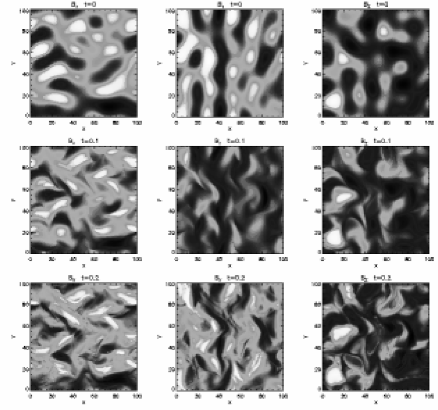
Figure 2: Plots of the $R_{B}=1000$ solution in real configuration space at $t=0$ (top row), $t=0.1$ (middle row) and $t=0.2$ (bottom row).The fields have been rescaled onto grids of $100\times 100$ points.

In Fourier space then, EMHD turbulence bears a strong resemblance to ordinary MHD turbulence. We would like to know if this resemblance carries over into real configuration space. In Figure 2, we show the three component fields at three times; the initial fields at $t=0$ (top row), intermediate fields at $t=0.1$ (middle row) and fully developed turbulent fields at $t=0.2$ (bottom row). In classical and MHD turbulence, a fully developed turbulent field in real configuration space would bear no resemblance to the initial field, but here the fields are much more structured and fully developed turbulent fields strongly resemble initial fields. This appears to be a unique characteristic of decaying EMHD turbulence.

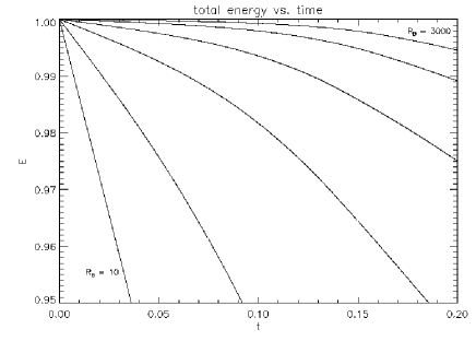
Figure 3: A plot of energy against time for $R_{B}=10$, 30, 100, 300, 1000 & 3000, increasing from left to right.

We would also like to address the energy decay of the field, with particular respect to any dependency of the decay rate on the value of $R_{B}$. Ref. Biskamp, Schwarz & Drake (1996) in the first study of 2D EMHD reported that the energy dissipation rate is independent of the value of the dissipation coefficient, represented by $R_{B}$ here. In contrast to this, we find that the energy decay is much slower at higher $R_{B}$, as plotted in Figure 3.

III.2 Large-scale initial conditions in the presence of a background field

EMHD turbulence, like classical and MHD turbulence, is isotropic when allowed to freely decay. In the presence of a background flow, classical turbulence remains isotropic since it is locally coupled in Fourier space. Small-scale structures are simply advected along by the large-scale flow, whether or not that has a uniform background contribution. Numerical simulations of MHD turbulence have found it to be strongly anisotropic in the presence of a background field Shebalin et al. (1983); Oughton et al. (1998). This has been attributed to the excitation of Alfvén waves which preferentially propagate parallel to the external magnetic field and hinder the cascade process perpendicular to the external field.

In EMHD turbulence, recent numerical studies employing hyperdiffusivity Dastgeer et al. (2000); Dastgeer & Zank (2003) have revealed similar strongly anisotropic behaviour. This can only be the result of asymmetry in the nonlinear spectral transfer process relative to the external magnetic field. In the context of local energy coupling in Fourier space, mediation by whistler waves has been proposed as the only way this asymmetry could be achieved Dastgeer et al. (2000) with the method detailed in ref. Galtier (2006). The spectrum of 2D anisotropic EMHD turbulence has also been shown to exhibit a linear relationship with an external magnetic field Dastgeer & Zank (2003).

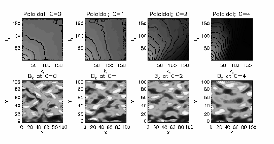
Figure 4: Fourier power spectra and real space fields at $t=0.2$ for 2D EMHD turbulence in the presence of a background field. We show 2D Fourier power spectra of $a$, the poloidal field, for $R_{B}=100$ at $C=0$, 1, 2 & 4 across the top row. Across the bottom row we show the corresponding B_x fields in real configuration space.

In order to understand how hyperdiffusivity has affected previous studies we have introduced a background field into the governing equations as discussed above and calculated solutions for $R_{B}=100$ & 300 at a spatial resolution of $512^{2}$ points in real configuration space. We present our results in Figure 4. Across the top row, we show 2D energy spectra for $R_{B}=100$ with $C=0$, 1, 2 & 4. In the isotropic case with no background field, i.e. $C=0$, energy is evenly distributed between $x$ and $y$, as indicated by circular contours. In the case of $C=1$ we find energy transfer to larger $k$ has been suppressed in the $x$ direction, parallel to the background field. EMHD turbulence has become anisotropic in the presence of a uniform background field with normal diffusivity. The effect becomes more pronounced for $C=2$ and $C=4$. The evolution of modes parallel and perpendicular to the field is clearly different, as the spectral cascade in the parallel wavenumbers is clearly suppressed. This suppression has been attributed to excitation of whistler waves, which act to weaken spectral transfer along the direction of propagation Dastgeer & Zank (2003). Across the bottom row, we show the corresponding $B_{x}$ fields. For $C=0$, the field is isotropic, but as the value of $C$ is increased, structures are stretched in the $x$ direction corresponding to increasingly inhibited energy transfer in $x$ but not in $y$, perpendicular to the field direction.

This result is in agreement with Cho & Lazarian (2004) who found scale-dependent anisotropy in numerical studies of 3D EMHD turbulence employing hyperdiffusivity. Our simulations also support the linear relationship between 2D EMHD turbulence and strength of external magnetic field found by Dastgeer & Zank (2003). At $R_{B}=300$ we reassuringly find the field is more anisotropic.

It is worth noting here that since (1) is scale invariant - we can apply the equation over the whole of a system, or just a small section, with $R_{B}$ unchanged - if you take a very small box, then this box will see the large-scale field as a background field, and therefore one would expect the smallest scales in the system, for example a neutron star, to be anisotropic.

III.3 Intermediate-scale initial conditions

In classical turbulence, the exchange of energy and enstrophy $\Omega$ is coupled in Fourier space according to

$$\frac{\partial E}{\partial t}=-k^{2}\frac{\partial\Omega}{\partial t},$$ (11)

hence energy injected at intermediate scales experiences a transfer to both higher and lower wavenumbers in order to satisfy this coupling and simultaneously conserve energy and enstrophy. This is the inverse cascade of energy to lower $k$ (larger scales) Kraichnan (1967). In MHD turbulence, energy and magnetic helicity are coupled in the same way and an inverse cascade occurs in order to simultaneously conserve these two quadratic ideal invariants. To investigate whether an inverse cascade occurs in decaying EMHD turbulence, we inject energy over the wavenumber range $10\leq k\leq 20$ as detailed above and evolve the magnetic field.

In Figure 5 we show the solution for $R_{B}=1000$ at various times. To fully resolve the solution in a reasonable amount of computational time we have chosen to evolve the field to $t=0.2$ at a resolution of $2048^{2}$ real space points, then to $t=1.0$ with $1024^{2}$ points and finally to $t=15.0$ with $512^{2}$ points. For this reason the energy spectra have different extents in Fourier space at the different times $t=0.0$ (dashed line), 0.1, 1.0, 3.0, 6.0, & 15.0. We include the full information, rather than just cutting off the plot at $k=100$, to demonstrate that our solutions are indeed fully resolved. The spectra show that energy is clearly transferred to $k<10$ in an inverse cascade, with the spectral peak shifting to $k=2$ but not maintaining the same amplitude. Some energy has also transferred to $k>20$ resulting in an overall spectrum comparable to a forward homogeneous cascade at late time. At $t=0.1$ the spectrum has a spectral index of -5/2 for $k>10$. At late time this has steepened to $\sim-3$. Between $t=12$ and $t=15$, the spectral index has stabilised. The inverse cascade phenomenon becomes less pronounced at lower values of $R_{B}$ with no inverse cascade at all below $R_{B}=300$.

In Figure 6 we show the evolution of the field by including the real configuration space fields at times $t=0.1$, 3.0 and 15.0. The initial field containing intermediate scale structure can be seen to develop large scale structures, which unlike ordinary or MHD turbulence again appear to be relatively stationary.

Previous work has considered inverse cascade action in driven, rather than decaying, 2D EMHD turbulence Shaikh & Zank (2005). There the authors found a forward cascade of energy and an inverse cascade of mean squared magnetic potential or anastrophy. Between the forcing lengthscale and the artificial dissipative cutoff, the authors found a $k^{-7/3}$ energy spectrum consistent with our results at $t=0.1$. It remains unclear though why the spectrum steepens at late time. Previous work Chertkov et al. (2007) has found a tendency toward energy condensation in forced 2D classical turbulence. There the condensation is a finite size effect of the biperiodic box which occurs after the standard inverse cascade reaches the size of the system. It leads to the emergence of a coherent vortex dipole. It is important to note that the dipole contains most of the injected energy and since we are simulating decaying EMHD turbulence, we do not inject any energy which could power the emergence of such a structure. The real field in Figure 6 shows no evidence of collimated dipole structure and in fact a large number of isolated vortices can be seen, a characteristic of fluid turbulence noted in Shaikh & Zank (2005). Here then we deduce we are seeing the first direct demonstration of the dual cascade phenomenon in decaying 2D EMHD turbulence.

IV Conclusions

We have investigated the nature of decaying 2D EMHD turbulence with normal diffusivity and compared it with classical and MHD turbulence and studies of 2D EMHD with hyperdiffusivity. We have found EMHD turbulence experiences an isotropic forward cascade of energy to higher wavenumber (smaller spatial scales) asymptotically approaching $E_{k}\propto k^{-5/2}$ with increasing $R_{B}$ (inversely proportional to a dissipation coefficient), in broad agreement with previous studies. We have found there is no dissipative cutoff at the predicted wavenumber $k\sim R_{B}^{4/5}$ and argue this is consistent with non-local coupling in Fourier space, the most important result of this paper. Hyperdiffusivity has previously clouded this issue and introduced an artificial cutoff. Only now, when we can avoid its use, has the true nature become clear. We have also found that fully developed EMHD turbulence appears to be strongly structured, retaining a similarity to the initial field at late time, very much unlike classical or MHD turbulence and a point not noted in previous literature. Our study of EMHD turbulence with normal diffusivity has been found to display scale-dependent anisotropy in the presence of a uniform background field, in good agreement with previous studies employing hyperdiffusivity. Further, our results support previous studies which found the strength of the anisotropy is linearly related to the external field strength. Finally, we have discovered that decaying EMHD turbulence is capable of yielding an inverse cascade, at least partially transferring magnetic energy from intermediate to large lengthscales. This result may be particularly significant for the magnetic fields of neutron stars, where the proto-neutron star that emerges from a supernova explosion may well have a primarily small-scale, disordered field. A Hall-induced inverse cascade may then be a mechanism whereby it acquires a large-scale, ordered field.

Acknowledgements We thank Steve Tobias for his assistance in benchmarking the code and an anonymous referee for their insightful comments enabling us to improve the paper. This work was supported by the Science & Technology Facilities Council [grant number PP/E001092/1].

Figure 5: Evolution of the Fourier power spectra for $R_{B}=1000$, showing an inverse cascade of energy to $k<10$. Spectra are shown at $t=0.0$ (dashed line), 0.1, 1.0, 3.0, 6.0 & 15.0. Note the changes in resolution from $N=2048$ at $t=0.1$ to $N=1024$ at $t=1.0$ to $N=512$ at later times.

Figure 6: Plots of the $R_{B}=1000$ solution in real configuration space at $t=0.1$ (top row), $t=3.0$ (middle row) and $t=15.0$ (bottom row). The fields have been rescaled onto grids of $100\times 100$ points.

References

- Goldreich & Reisenegger (1992) P. Goldreich, A. Reisenegger, Astrophys. J. 395, 250 (1992).
- Hollerbach & Rudiger (2002) R. Hollerbach, G. Rüdiger, Mon. Not. Roy. Astron. Soc. 337, 216 (2002).
- Biskamp, Schwarz & Drake (1996) D. Biskamp, E. Schwarz, J.F. Drake, Phys. Rev. Lett. 76, 1264 (1996).
- Biskamp et al. (1999) D. Biskamp, E. Schwarz, A. Zeiler, A. Celani, J. Drake, Phys. Plasmas 6, 751 (1999).
- Dastgeer et al. (2000) S. Dastgeer, A. Das, P. Kaw, P. Diamond, Phys. Plasmas 7, 571 (2000).
- Dastgeer & Zank (2003) S. Dastgeer, Zank G.P., Astrophys. J. 599, 715 (2003).
- Cho & Lazarian (2004) J. Cho, A. Lazarian, Astrophys. J. 615, L41 (2004).
- Shaikh & Zank (2005) Sheikh D., Zank G.P., Phys. Plasmas 12, 122310 (2005)
- Frigo & Johnson (2005) M. Frigo, S.G. Johnson, Proc. of the IEEE 93, 216 (2005).
- Berger (1997) M.A. Berger, J. Geophysical Research 102, 2637 (1997).
- Kolmogorov (1941) A.N. Kolmogorov, Proc. USSR Acad. Sciences 30, 299 (1941) (Russian). Proc. Roy. Soc. A 434, 9 (1980) (English).
- Kraichnan & Montgomery (1980) R.H. Kraichnan, D. Montgomery, Rep. Prog. Phys. 43, 547 (1980).
- Shebalin et al. (1983) J.V. Shebalin, W.H. Matthaeus, D. Montgomery, J. Plasma Phys. 29, 525 (1983).
- Oughton et al. (1998) S. Oughton, W.H. Matthaeus, S. Ghosh, Phys. Plasmas 5, 4235 (1998).
- Galtier (2006) S. Galtier, J. Plasma Phys. 72, 721 (2006).
- Kraichnan (1967) R.H. Kraichnan, Phys. Fluids 10, 1417 (1967).
- Chertkov et al. (2007) M. Chertkov, C. Connaughton, I. Kolokolov, V. Lebedev, Phys. Rev. Lett. 99, 084501 (2007).