Traffic and the visual perception of space

Abstract

During the attempt to line up into a dense traffic people have necessarily to share a limited space under turbulent conditions. From the statistical point view it generally leads to a probability distribution of the distances between the traffic objects (cars or pedestrians). But the problem is not restricted on humans. It comes up again when we try to describe the statistics of distances between perching birds or moving sheep herd. Our aim is to demonstrate that the spacing distribution is generic and independent on the nature of the object considered. We show that this fact is based on the unconscious perception of space that people share with the animals. We give a simple mathematical model of this phenomenon and prove its validity on the real data that include the clearance distribution between: parked cars, perching birds, pedestrians, cars moving in a dense traffic and the distances inside a sheep herd.

1 Introduction

Everyone knows that to park a car in the city center is problematic. The amount of the available places is limited and it has to be shared between too many interested parties. Birds face the same problem when a flock tries to perch on an electric line. Similar reasons lead also to the troubles in the highway traffic, to the pedestrian queues and so on. For instance the unpopular transport jams are a consequence of the car-car interaction in a regime of a high car density.

The interaction is basically evoked by the brain activity and mediated through the muscles (pedestrians) or accelerator/brake pedals (cars). In both cases it is the brain that is responsible for the interaction. So it should be not surprising that the phenomena observed for cars and pedestrians are similar. Even more: the spatial perception is evolutionary very old and people share it with animals. So we should be not surprised to find the same results also when dealing with animal herds instead of human traffic. Anyhow: a deeper understanding of the related processes is of interest and will be discussed here.

The attempt to describe the intrinsic and basically unconscious mechanisms used by the human brain on the basis of their everyday activity is not new. It goes back at least to the celebrated work of G.K. Zipf [1] describing the universal features of languages. The concept was worked out in detail by the sociologist H. A. Simon, within a set of assumptions which became known as the Simon s model [2], see also [3] for the recent results in musicology.

The subjects of our study (parking, car transport, pedestrian dynamics, herd and flock dynamics) were treated separately in the past. The random car parking model was introduced by Renyi [4] (see [5], [6] for review) and compared with the data collected on the street in [7], [8]. Other models describe the car transport on highways - see for instance [10] and [9] for review. Another approach is used for the pedestrian dynamics utilizing social forces - see [11]. For the dynamics of a starling flock see [12] and [13]

Our aim is to present a simple theory based on the visual perception that is capable to describe all the observed facts regardless whether they originate from cars, pedestrians or animals. The perception mechanism is very old and therefore shared by many species ranging from insects to mammals. For humans it is processed automatically and without the conscious control. We will use it to understand the statistical properties of the distances between the neighboring competitors (cars, pedestrians, birds and sheeps) in a situation when the available space is limited. .

The paper is organized as follows: In the Section 2 we describe the mathematical model and derive a one parameter family of possible distance distributions. Section 3 contains the psychophysical background of the distance control based on the unconsciously evaluated time to collision with the neighbor. The Section 4 contains the comparison of the theory with the collected data.

2 Dividing the available space

To illustrate the approach we focus on the spacing distribution (bumper to bumper distances) between cars parked in parallel. The generalization of the method to other situations will be discussed at the end of this section.

We will assume that the street segment used for parking starts and ends with some clear and non-transportable part unsuitable for parking. It can be a driveway or a turning to the side street. Otherwise the parking segment is free of any kind of obstructions. We will assume that it has a length $L$ and is free of any kind of marked parking lots or park meters. So the drivers are free to park the car anywhere in the segment provided they find an empty space to do it. We suppose also for simplicity that all cars have the same length $l_{0}$. Since many cars are cruising for parking there are not free parking lots and a car can park only when another parked car leaves. To simplify the further formulation of the problem and to avoid troubling with the boundary effects we assume that the street segment under consideration forms a circle. The car spacing distribution is obtained as a steady solution of the repeated car parking and car leaving process.

To park a car of the length $l_{0}$ one needs (due to the parking maneuver) a lot of a length larger then $\approx 1.2l_{0}$. So in a segment of the length $L$ the number of the parked cars equals to $N\approx[L/(1.2l_{0})]$. Denoting by $D_{k}$ the spacing between the car $k$ and $k+1$ we get $\sum_{k=1}^{N}D_{k}=L-Nl_{0}$ and after a simple rescaling finally

$$\sum_{k=1}^{N}D_{k}=1.$$ (1)

Since all lots are occupied the number of the parked cars is supposed to be fixed. The repeated car leaving and car parking reshuffles however the distances $D_{k}$. We will treat them as independent random variables constrained by the simplex (1). The distance reshuffling goes as follows: In the first step one randomly chosen car leaves the street and the two adjoining lots merge into a single one. In the second step a new car parks into this empty space and splits it again into two smaller lots. The related equations are simple. If a car leaves the neighboring spacings - say the spacings $D_{n},D_{n+1}$ - merge into a single lot $D$:

$$D=D_{n}+D_{n+1}+l_{0}.$$ (2)

When a new car parks to $D$ it splits it into $\tilde{D}_{n},\tilde{D}_{n+1}$:

$$\tilde{D}_{n} = a(D-l_{0})$$

$$\tilde{D}_{n+1} = (1-a)(D-l_{0}).$$ (3)

where $a\in(0,1)$ is a random variable with a probability density $q(a)$. The distribution $q(a)$ describes the parking preference of the driver. We assume that all drivers share the same $q(a)$. (The meaning of the variable $a$ is straightforward. For $a=0$ the car parks immediately in front of the car delimiting the parking lot from the left without leaving any empty space. For $a=1/2$ it parks exactly to the center of the lot $D$ and for $a=1$ it stops exactly behind the car on the right.) Combining (2) and (3) gives finally the distance reshuffling

$$\tilde{D}_{n} = a(D_{n}+D_{n+1})$$

$$\tilde{D}_{n+1} = (1-a)(D_{n}+D_{n+1}).$$ (4)

and the car length $l_{0}$ drops out. The simplex (1) is of course invariant under this transformation.

For various choices of $n$ the mappings (4) are regarded as statistically independent. Since all cars are equal the joint distance probability density $P(D_{1},...,D_{N})$ has to be exchangeable ( i.e. invariant under the permutation of the variables) and invariant with respect to (4). Its marginals $p_{k}(D_{k})$ (the probability density of a particular spacing $D_{k}$) are identical:

$$p_{k}(D_{k})=p(D_{k})=\int_{D_{1}+..+D_{N}=1}P(D_{1},...,D_{N})dD_{1}..dD_{k-1}dD_{k+1}..dD_{N}.$$ (5)

A standard approach to deal with the simplex (1) is to take $D_{k}$ as independent random variables normalized by a sum:

$$D_{k}=\frac{d_{k}}{\sum_{n=1}^{N}d_{n}}.$$ (6)

where $d_{k}$ are statistically independent and identically distributed. Moreover: it is obvious that the distribution of $\{D_{1},..,D_{N}\}$ is invariant under the transform (4) merely when the distribution of $\{d_{1},..,d_{N}\}$ is invariant. The relation (4) reads for the variables $d_{n}$:

$$\tilde{d}_{n} = a(d_{n}+d_{n+1})$$

$$\tilde{d}_{n+1} = (1-a)(d_{n}+d_{n+1})$$ (7)

($a,d_{n},d_{n+1}$ are now statistically independent and $d_{n},d_{n+1}$ are identically distributed).

The parking maneuver is regarded as known and described by the distribution $q(a)$. For simplicity we assume a symmetric maneuver, i.e. $q(a)=q(1-a)$. This means that the drivers are not biased to park more closely to a car adjacent from the behind or from the front. With given $q(a)$ we look for the distribution of $d_{n}$ that is invariant under the transform (7). In other words the effort is to solve the equation

$$d\triangleq a(d+d^{\prime})$$ (8)

where $d^{\prime}$ is an independent copy of the variable $d$ and the symbol $\triangleq$ means that the left and right hand sides of (8) have identical statistical properties.

Distributional equations of this type are mathematically well studied - see for instance [14] - although not much is known about their exact solutions. In particular it is known that for a given distribution $q(a)$ the equation (8) has an unique solution that can be obtained numerically by iterations. We are however interested in an explicit result. We restrict therefore the possible densities $q(a)$ to a two parametric class of the standard $\beta$ distributions. Then the solution of (8) results from the following statement [15]:

Statement: Let $d_{1},d_{2}$ and $a$ be independent random variables with the distributions: $d_{1}\sim\Gamma(a_{1},1)$, $d_{2}\sim\Gamma(a_{2},1)$ and $a\sim\beta(a_{1},a_{2})$. Then $a(d_{1}+d_{2})\sim\Gamma(a_{1},1)$.

The symbol $\sim$ means that the related random variable has the specified probability density. $\Gamma(g,1),\beta(g_{1},g_{2})$ denote the standard gamma and beta distributions respectively.

For a symmetric parking maneuver $g_{1}=g_{2}=g$. The variables $d_{1},d_{2}$ are then equally distributed and the solution of (8) reads $d\sim\Gamma(g,1)$. The relation (6) returns the spacings $D_{k}$. We find that the joint probability density $P(D_{1},...,D_{N})$ is nothing but a one parameter family of the multivariate Dirichlet distributions on the simplex (1) [16]:

$$P(D_{1},...,D_{N})=\frac{\Gamma(Ng)}{\Gamma(g)^{N}}D_{1}^{g-1}D_{2}^{g-1}...D_{N}^{g-1}$$ (9)

Its marginal (5) is simply $D\sim\beta(g,(N-1)g)$. Normalizing the mean of $D$ to $1$ we are finally left with

$$p(D)=\frac{1}{N}\beta\left(g,(N-1)g,\frac{D}{N}\right).$$ (10)

A similar reasoning applies also for the moving cars. Assume a sequence of cars in a high density traffic. All the cars move with similar velocity and with the mutual distances $D_{k}$. In course of the traffic flow the driver of the car $k$ tries to optimize his position. He can overtake the car $k+1$ or update the distances to the neighboring cars $k-1$ and $k+1$. In doing so he uses the same mechanism as for parking. The only difference is that in the traffic flow we assume the existence of certain safety margin. So the update mapping reads now

$$\tilde{D}_{n} = d+a(D_{n}+D_{n+1}-2d)$$

$$\tilde{D}_{n+1} = d+(1-a)(D_{n}+D_{n+1}-2d).$$ (11)

where $d$ is the safety margin representing the minimal distance. For maneuvers related with the approach to a standing object (like the parking maneuver) we set $d=0$. In the course of a car-following in a dense traffic the value of $d$ reflects the reaction time of the driver and his velocity. Changes in the driving situation like night versus day conditions affect this component. We will however neglect this fact and regard $d$ as a constant. For experimental results describing the value of $d$ under various conditions see for instance [17].

We assume that outside the safety margin the driving strategy is identical with that of the parking. So in a steady traffic flow the distribution of the distances $D_{k}-d$ has to conforms with the distribution obtained for the car parking.

The cars are of course not somehow extraordinary. The same reasoning applies for pedestrians, animals in a herd and so on. In all cases the distribution $q(a)$ is crucial. We will argue that $q(a)$ is related to the inborn visual perception of the distance and independent on the "hardware" actually used to realize the motion.

3 Distance perception

The ranging maneuver is described by the probability density $q(a)$ and defined by the relation (4). To ensure a solvability we restricted the possible maneuvers to $q(a)=\beta(g,g,a)$, with $g$ being a free parameter. We will now demonstrate that the natural choice is $g=3$.

The point is that for small $a$ the behavior of $q(a)$ reflects the capability of the driver/pedestrian/animal to estimate small distances. The collision avoidance during the ranging is guided visually. We assume that the same visual ability is shared by all participants. If this applies the behavior of $q(a)$ for small $a$ has to be generic, i.e. independent on the particular situation. It is fixed merely by the perception of the distance.

A distance perception is a complex task and there are several cues for it. Some of them are monocular (linear perspective, monocular movement parallax etc.), others oculomotor (accommodation convergence) and finally binocular (i.e. based on the stereopsis). In human all of them work simultaneously and are reliable under different conditions - see [18] for more details. For the ranging however the crucial information is not the distance itself but the estimated time to collide with the neighbor which has to be evaluated using the knowledge of the mutual distance and velocity.

It has been argued in a seminal paper by Lee [19] that the estimated time to collision is psychophysically derived using a quantity defined as the inverse of the relative rate of the expansion of a retinal image of the moving object (this rate is traditionally denoted as $\tau$). Behavioral experiments have indicated that $\tau$ is indeed controlling actions like contacting surfaces by flies, birds and mammals (including humans): see [20],[21],[22]. Moreover the studies have provided abundant evidence that $\tau$ is processed by specialized neural mechanisms in the the retina itself and in the brain [23]. The hypothesis is that $\tau$ is the informative variable for the collision free motion - see [24] for review.

Let $\theta$ be the instantaneous angular size of the observed object (for instance the front of the car we are backing to during the parking maneuver). Then the estimated time to contact is given by

$$\tau=\frac{\theta}{d\theta/dt}$$ (12)

Since $\theta(t)=2\arctan(L_{0}/2D(t))$ with $L_{0}$ being the width of the approached object and $D(t)$ its instantaneous distance, we get

$$\tau(t)=-\frac{L_{0}^{2}+4D(t)^{2}}{2L_{0}(dD(t)/dt)}\arctan\left(\frac{L_{0}}{2D(t)}\right).$$ (13)

For $D>>L_{0}$ and a constant approach speed $v=-dD/dt$ the quantity $\tau$ simply equals to the physical arrival time: $\tau=D/v.$ For small distances, however, $\tau\approx D^{2}/(vL_{0})$ and the estimated time to contact decreases quadratically with the distance. (Note that $\tau$ gives the arrival time without explicitly knowing the mutual velocity, the size of the object and its distance.)

We assume that the probability to exploit small distances is proportional to the estimated time to contact . This means in particular that if $\tau$ evaluated in the course of an approach is small (i.e. a collision is impending) the maneuver is stopped. Based on this principle we get for small distances $p(D)\approx D^{2}$ and from 3 finally $q(a)\approx a^{2}$ for small $a$. Since $q(a)=\beta(g,g,a)$ this sets the parameter $g$ to $g=3$. The normalized clearance distribution (10) reads simply

$$p(D)=\frac{1}{N}\beta\left(3,3(N-1),\frac{D}{N}\right)=\left(\frac{1}{N}\right)^{3(N-1)}\frac{\Gamma(3N)}{2\Gamma(3(N-1))}D^{2}(N-D)^{3N-4}$$ (14)

The described mechanism works so to say in the background, i.e. without being conscious. Moreover: $\tau$ is evaluated equally by humans and by animals. We will show in the next section that this fact leads to an universality in their behavior.

4 The measured data

The estimation of the distance $D$ through $\tau$ leads simply to $p(D)\approx D^{2}$ for small $D$. So let us first check the validity of this relation. There exist a simple observation that enables us to do it: the car stopping on a crossing equipped with traffic lights. If the light is red the cars stop and form a queue. We assume that the drivers stop independently and in a distance to the preceding car that is evaluated by $\tau$. So the clearance statistics should give an evidence of the validity of the $\tau$ hypothesis. There was also a direct experiment measuring the clearance statistics in laboratory conditions - see [25],[26].

We photographed the car queues in a front of the red light. The photographes were taken all from one spot and at the same daytime. The clearances were finally obtained by digitalization. Altogether we extracted 1000 car distances from one particular crossing in the city of Hradec Kralove (Czech republic) and evaluated the corresponding probability density $p(D)$. Similar measurement has been done also on several crossings in Prague - see [27]. If there is a linear correlation between the stopping distance and the estimated time to contact $\tau$ the obtained distance density $p(D)$ should behave as $\approx D^{2}$ for small $D$. The result for small distances is plotted on the Figure 1. It shows a very nice agreement with that assumption.

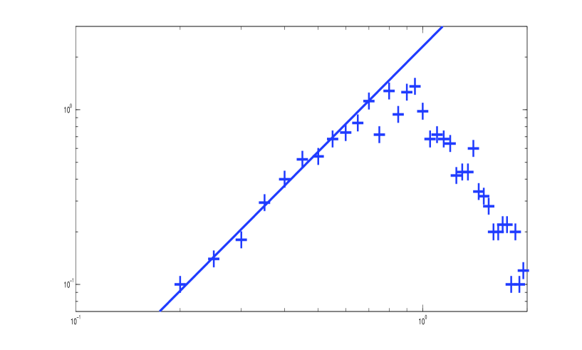
Figure 1: The probability density $p(D)$ evaluated for the measured data (crosses) is in a log-log scale compared with the function $2.3*D^{2}$ (full line). The agreement for small $D$ is evident.

To show that the $\tau$ mechanism is generic leading to a distance distribution that is independent on the objects (the object can be a man, animal or a car) we divide the further observations into two categories: the first contains sedentary objects and the second object moving in a dense environment.

Let us start with the the clearance distribution obtained for cars parked in parallel and for birds perching on a power line. In both cases the "parking segment" is full, i.e. there is not a free space to place an additional participant. We have argued that under this conditions the resulting distribution is invariant under the transform (7) with the parameter $g$ in (10) fixed to $3$. The "parking" segments under consideration were long and containing a large number of objects. So $N>>1$, and the constrain (1) does not play a substantial role. In this case $p(D)$ equals to $\Gamma(3,1,D)$.

To verify the prediction we measured the bumper to bumper distances between cars parked in the center of Hradec Kralove (Czech Republic). The street was located in a place with large parking demand and usually without any free parking lots. Moreover it was free of any dividing elements, side ways and so on. Altogether we measured 700 spacings under this conditions.

For the birds we photographed flocks of starlings resting on the power line during their flight to the south. The line was "full", i.e. other starlings from the flock were forced to use another line to perch. The bird-to-bird distances were obtained by a simple digitalization - altogether 1000 bird spacings. After scaling the mean distance to 1 the results were plotted on the Figure 2 and compared with the prediction (10).

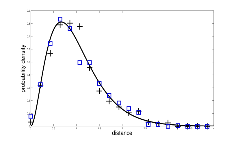
Figure 2: The probability density of the distances between the parked cars (crosses) and perching starlings (squares) is compared with the prediction of the theory (full line). The mean distance is normalized to 1.

The probability distributions resulting from these data seems to be (up to the statistical fluctuations) identical and in a good agreement with the model prediction. This is amazing since the used "hardware" is fully different. The underlying psychophysical mechanism for the time to contact estimation, is, however, identical. (For the experimental results concerning the relevance of $\tau$ for the space perception of pigeons see [28].)

Let us now pass to the traffic streams, i.e. to a situation when the objects are collectively moving. We assume a dense traffic. The distances between the moving objects are small and have to be constantly controlled to avoid possible collisions. We use the mapping (11).

Outside the safety margin the collision avoidance is assumed to be based on $\tau$. This means that the distribution of the distances $D_{k}-d$ follows the mapping (7) with the same probability density $q(a)$ as in the "parking" case. So the distributions of $D_{k}-d$ should be universal.

In order to verify this hypothesis we organized a simple experiment with pedestrians in a narrow corridor. Using two light gates we measured their velocity and the time interval that elapsed between two subsequent walkers. This enables us to reconstruct the mutual distances and evaluate the distance probability density. The same device and method was used also for a sheep herd moving through an aisle between two near yards. The third source of data are cars moving on a highway in a dense traffic. The velocity and time stamps of the individual cars were obtained by induction loops placed below the roadway.

The safety margins $d$ are clearly different in these three cases and we removed them by subtracting the minimal distance from the given data set. The mean distance was finally normalized to 1. The result is plotted on the figure 3

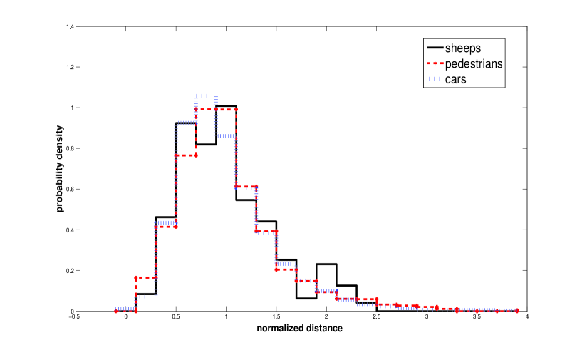
Figure 3: The probability density of the distances between the cars on highway in a high density regime, pedestrians walking in a narrow corridor and sheeps moving in an aisle between two barriers is plotted. The minimal distance on each particular data set is subtracted and the mean distance is normalized to 1.

Again: the resulting distance distribution is universal and in agreement with the theory based on $\tau$ hypothesis.

To summarize we have demonstrated that the clearance between objects (cars,pedestrians,birds and sheeps) is largely universal. This surprising observation can be understood as a consequence of an universal distance controlling mechanism shared by human and animals.

Acknowledgement: The research was supported by the Czech Ministry of Education within the project LC06002. The help of the PhD. students of the Department of Physics, University Hradec Kralove who collected the majority of the data is gratefully acknowledged. The help of Shinya Okazaki which was responsible for the traffic light data is also gratefully acknowledged.

References

- [1] Zipf G. K., The Psycho-Biology of Language (Houghton-Mifflin, Boston, 1935).
- [2] Simon, H. A., Biometrika 42,(1955) 425 - 440 .
- [3] Zanette, D. H., Musicae Scientiae 10,(2006) 3 - 18 .
- [4] Renyi A.: Publ. Math. Inst. Hung. Acad. Sci. 3 (1958) 109.
- [5] Evans J.W.: Rev.Mod.Phys. 65 (4) (1993) 1281 - 1330
- [6] Cadilhe A.,, Araujo N.A.M. and Privman V.: J.Phys. Cond. Mat. 19 (2007) 065124
- [7] Rawal S., Rodgers G.J.: Physica A 246 (2005) 621 - 630
- [8] Seba P.: J.Phys.A 41 (2008) 122003
- [9] Chowdhury D., Santen L. and Schadschneider A.: Physics Reports (329) 4-6 (2000), 199-329
- [10] Kerner B.S.: Phys. Rev. Lett. 81 (1998) 3797
- [11] Schreckenberg M. and Sharma D.S. (eds.) Pedestrian and Evacuation Dynamics (Springer, Berlin 2002).
- [12] Ballerini M. at al: Proc.Nat.Acad.Sci. 105 (4) (2008) 1232 - 1237
- [13] Ballerini M. at al: An empirical study of large, naturally occurring starling flocks: a benchmark in collective animal behavior; arXiv:0802.1667 [q-bio]
- [14] Devroye L. and Neininger R.: Advances of Applied Probability, vol. 34 (2002) 441-468.
- [15] Dufresne D.: Adv. Appl. Math. 20 (1998) 285 - 299
- [16] Wilks, S.S.: Mathematical Statistics. John Wiley Sons, New York
- [17] Zhonghai Li and Paul Milgram: An empirical investigation of the influence of perception of time-to-collision on gap control in automobile driving. Proceedings of the human factors and ergonomics society 48th annual meeting 2004, page 2271- 2275
- [18] Jacobs R.A.: Trends in Cognitive Sciences Vol.6 No.8 (2002) 345
- [19] Lee, D. N.: A theory of visual control of braking based on information about time-to-collision. Perception 5 (1976), 437 - 459.
- [20] van der Weel F.R., van der Meer L.H., Lee N.D.: Human Movement Science 15 (1996) 253-283
- [21] Hopkins B.,Churchill A., Vogt S., Ronnqvist L.: Journal of Motor Behavior 36, Number 3 (2004) 3 - 12
- [22] Schrater P.R., Knill D.C., Simoncelli E.P.: Nature 410 (2001) 816
- [23] Farrow K., Haag J. and Borst A.: Nature Neuroscience 9 (2006) 1312 - 1320
- [24] Fajen B.R.: Journal of Experimental Psychology 31, No. 3 (2005) 480 - 501
- [25] Gadgil S. and Green P.: How much clearance drivers want while parking: data to gude the design of parking assistance systems. In PROCEEDINGS of the HUMAN FACTORS AND ERGONOMICS SOCIETY 49th ANNUAL MEETING 2005, 1935-1940
- [26] Green, P., Gadgil, S., Walls, S., Amann, J., and Cullinane, B. (2004). Desired Clearance Around A Vehicle While Parking or Performing Low Speed Maneuvers. (Technical Report UMTRI 2004-30), Ann Arbor, Michigan: University of Michigan Transportation Research Institute.
- [27] Krbalek M.: J. Phys. A: Math. Theor. 41 (2008), 205004
-
[28]
Hong-Jin Sun, Jian Zhao, Southall T. L. and Bin Xu: Visual
Neuroscience (2002), 19, 133 - 144.
Hongjin Sun and Frost B.J.: Nature Neuroscience 1 (4) (1998) 296
Hongjin Sun and Frost B.J.: in Time-to-Contact, Advances in Psychology, Heiko Hecht, Geert J. P. Savelsbergh (Eds.) 2003 Amsterdam: Elsevier - North-Holland