Extended solutions via the trial-orbit method for two-field models

Abstract

In this work we investigate the presence of defect structures in models described by two real scalar fields. The coupling between the two fields is inspired on the equations for a multimode laser, and the minimum energy trivial configurations are shown to be structurely dependent on the parameters of the models. The trial orbit method is then used and several non-trivial analytical solutions corresponding to topological solitons are obtained.

The study of topological defects is a well established field, particularly for models described by scalar fields raj1 ; msu . The simplest topological defect - the kink - arises in theories of scalar fields in two-dimensional space-timerub . For usual models with spontaneous breaking of global symmetry, such defects interpolate between two minima of the potential. Important examples in condensed matter physics are the well-known domain walls, which separate regions of different magnetization. These defects are essentially classical objects with localized and stable distribution of density energy. In the case of two coupled real scalar fields, the equations of motion are very hard to solve due to non-trivial nonlinearities. However, there are interesting situations where real progress have been done – see, e.g. Refs.t1 ; t2 ; t3 ; t4 ; t5 ; t6 .

In 1979, Rajaraman proposed a method to solve the pair of equations of motion which usually appear in models described by two real scalar fields t4 : it is named the trial orbit method, which relies on the search (in a trial way approach) for an appropriate orbit the two fields have to obey in the two-dimensional configuration space. Eventually, when one tries the right orbit, we can be able to solve the problem analytically. However, since the equations of motion are second order differential equations, the task of finding exact solutions is very hard and the trial orbit method is not much efficient.

Some years before - in 1976 - an interesting work bog identified an important class of models, showing how to reduce the equations of motion to a system of first order differential equations. In 1995, this subject was studied by one of us in ref. bsr , that is, the Rajaraman’s trial orbit method t4 was applied for the first order equations obtained within the Bogomol’nyi procedure bog . The use of the trial orbit method for first order differential equations was shown to be very efficient and this new procedure allowed us to make interesting progress, as it is shown in bb and in references therein. More recently the use of the trial orbit method for models whose equations of motion can be reduced to first order differential equations was systematized in bflr . Other investigations on similar issues have also been done in refb -d , which use distinct procedures and motivations to study two-field and other related models.

In the case of a model with two fields, the kink-like solutions are orbits in the field space. In this work, we will further explore the trial orbit method to investigate models described by first order equations. Here, although, we construct a class of models inspired in a semiclassical theory of multimode laser and use the trial orbit method to find exact solutions that minimize the energy of the field configurations. The results show that, under certain conditions on the parameters of the system, several possible solutions connecting distinct minima of the models exist.

We consider a class of models in (1,1) Minkowski space-time dimensions described by the relativistic Lagrange density

$${\mathcal{L}}=\frac{1}{2}\partial_{\mu}\phi_{1}\partial^{\mu}\phi_{1}+\frac{1}{2}\partial_{\mu}\phi_{2}\partial^{\mu}\phi_{2}-V(\phi_{1},\phi_{2})$$ (1)

where $\phi_{1}$ and $\phi_{2}$ are the two real scalar fields, and we use the metric such that $x^{0}=x_{0}=t$ stands for the time, while $x^{1}=-x_{1}=x$ represents the spatial coordinate. The notation is usual for relativistic theories, with upper (lower) $\mu$ standing for contravariant (covariant) coordinates. The metric tensor is a diagonal $2\times 2$ matrix, compactly written as $g_{\mu\nu}=(1,-1)$. The Euler-Lagrange equation,

$$\partial_{\mu}\frac{\partial\mathcal{L}}{\partial(\partial_{\mu}\phi)}-\frac{\partial\mathcal{L}}{\partial\phi}=0$$ (2)

leads to the following equations of motion:

$$\frac{\partial^{2}\phi_{1}}{\partial t^{2}}-\frac{\partial^{2}\phi_{1}}{\partial x^{2}}+\frac{\partial V}{\partial\phi_{1}} = 0$$ (3a)

$$\frac{\partial^{2}\phi_{2}}{\partial t^{2}}-\frac{\partial^{2}\phi_{2}}{\partial x^{2}}+\frac{\partial V}{\partial\phi_{2}} = 0$$ (3b)

We are interested in kink-like solutions, which are described by static fields - $$\phi_{1}=\phi_{1}(x) \phi_{2}=\phi_{2}(x)$$, - so that

$$\frac{d^{2}\phi_{1}}{dx^{2}}=\frac{\partial V}{\partial\phi_{1}};\;\;\;\;\;\;\;\;\;\;\frac{d^{2}\phi_{2}}{dx^{2}}=\frac{\partial V}{\partial\phi_{2}}$$ (4)

In general, these equations are very hard to solve, but this task may be simplified if it is possible to replace these second order equations by first order differential equations. In order to get first order equations, we suppose that the potential is given in terms of another function, $W=W(\phi_{1},\phi_{2}),$ as bellow:

$$V(\phi_{1},\phi_{2})=\frac{1}{2}\left(\frac{\partial W}{\partial\phi_{1}}\right)^{2}+\frac{1}{2}\left(\frac{\partial W}{\partial\phi_{2}}\right)^{2}$$ (5)

In this case, the Bogomol’nyi method allows to argue that the solutions of the first order equations

$$\frac{d\phi_{1}}{dx}=\frac{\partial W}{\partial\phi_{1}};\;\;\;\;\;\;\;\;\;\;\frac{d\phi_{2}}{dx}=\frac{\partial W}{\partial\phi_{2}}$$ (6)

are also solutions of Eqs. (4), as it can be easily verified.

The potential of the above model has zeroes at the singular points of $W(\phi_{1},\phi_{2})$, and this set of singular points forms the vacua manifold of the field theory under investigation. Usually, distinct pairs of minima define distinct topological sectors of the model, and the solutions of the first order equations are defect structures with an energy cost given by $E=|\Delta W|,$ where

$$\Delta W=W(\phi_{1}(+\infty),\phi_{2}(+\infty))-W(\phi_{1}(-\infty),\phi_{2}(-\infty))$$ (7)

with the points $(\phi_{1}(+\infty),\phi_{2}(+\infty))$ and $(\phi_{1}(-\infty),\phi_{2}(-\infty))$ identifying minima in the vacua manifold. Since the energy density of the static fields is given by

$$\epsilon(x)=\frac{1}{2}\left(\frac{d\phi_{1}}{dx}\right)^{2}+\frac{1}{2}\left(\frac{d\phi_{2}}{dx}\right)^{2}+\frac{1}{2}\left(\frac{\partial W}{\partial\phi_{1}}\right)^{2}+\frac{1}{2}\left(\frac{\partial W}{\partial\phi_{2}}\right)^{2}$$ (8)

the energy is always positive, and the solutions which obey the first order equations are the minimum energy configurations in each topological sector of the model.

To be specific, let us now consider the superpotential

$$W=\frac{1}{2}\mu_{1}\phi_{1}^{2}+\frac{1}{2}\mu_{2}\phi_{2}^{2}-\frac{1}{4}\lambda_{11}\phi_{1}^{4}-\frac{1}{4}\lambda_{22}\phi_{2}^{4}-\frac{1}{2}\lambda_{12}\phi_{1}^{2}\phi_{2}^{2}$$ (9)

This choice represents a class of models described by the two sets of parameters: $\{\mu_{1},\mu_{2}\},$ and $\{\lambda_{11},\lambda_{22},\lambda_{12}\},$ the first being mass parameters while the second specifying interactions between the two fields. This potential implies the following first order differential equations:

$$\frac{d\phi_{1}}{dx} = (\mu_{1}-\lambda_{11}\phi_{1}^{2}-\lambda_{12}\phi_{2}^{2})\phi_{1}$$ (10a)

$$\frac{d\phi_{2}}{dx} = (\mu_{2}-\lambda_{21}\phi_{1}^{2}-\lambda_{22}\phi_{2}^{2})\phi_{2}$$ (10b)

where we have set $$\lambda_{21}=\lambda_{12}$$.

The present model represents in reality a family of models which is refereed to it some generality. Moreover, there is another specific motivation to adopt it: the system of Eqs. (10) is connected with the semiclassical theory of the laser and can simulate the competition between two adjacent modes in a cavity above the threshold (nuss , pp.126-131). It is said that the laser is at threshold when the pumping rate from the lower state to the upper excited state is just sufficient to overcome the cavity loss. In this way, for the particular case of a two-mode laser, within the approximation that the induced transition rate is well below the saturation rate, we have (note the resemblance with Eqs. (10a)-(10b)):

$$\dot{E_{n}}=\mu_{n}E_{n}-\lambda_{nn}E_{n}^{3}-\sum_{m\neq m}\lambda_{nm}E_{n}E_{m}^{2},n=1,2$$ (10c)

Here $E_{n}$ is the time-dependent slow-varying amplitude associated with the mode n, after expanding the electric field in the cavity in terms of a complete set of axial modes. With this motivation, the parameters $\mu_{1}$ and $\mu_{2}$ represent the overall gain, with the condition $\mu_{i}\geq 0$ being necessary to establish the laser oscillation in the mode i ($i=1,2$). Furthermore, $\lambda_{11}$ and $\lambda_{22}$ are saturation parameters, and one must have $\lambda_{ii}>0$ for positive population inversion of the mode $i$. The parameter $\lambda_{12}$ stands for the nonlinear saturation effect on the coupling between the two modes. We also have for the two-mode laser $\lambda_{12}\sim\lambda_{21}>0$. The study of competition among modes considers the analysis of the stability of the stationary solutions in a phase space diagram of $E_{1}^{2}$ versus $E_{2}^{2}$, where numerical solutions for arbitrary initial conditions reveal the stable and unstable points. It is found that stability of solutions is strongly dependent on the parameters, where one can have laser oscillation in just one of the modes or a simultaneous oscillation is both modes.

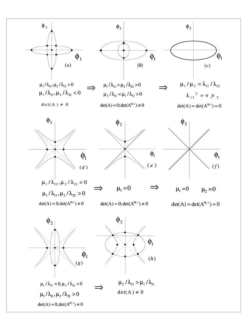
Figure 1: Diagrams showing all the possible minimum energy points.

Our work considers a similar problem. However, instead of investigate $\phi_{1}^{2}$ and $\phi_{2}^{2}$ in a phase space diagram, we follow another route and make an analysis in connection with the field description, searching for analytical description of the fields $\phi_{1}$ and $\phi_{2}$. To make the work as general as possible, let us start considering the vacua manifold, e.g. searching for all the possible minimum energy points of the potential, the critical points of $W.$ Initially we can count five points $(\phi_{1},\phi_{2})$ of minima: $(0,0),(\pm\phi_{1}^{\ast},0)$,$(0,\pm\phi_{2}^{\ast})$ with $\phi_{1}^{\ast}=\sqrt{\mu_{1}/\lambda_{11}}$ and $\phi_{2}^{\ast}=\sqrt{\mu_{2}/\lambda_{22}}$ – see Fig. 1. The case where both $\phi_{1}$ and $\phi_{2}$ are non vanishing can lead to 4 more points of minima, a continuum of points or no more points, depending on the relation between the parameters. We use the first order equations (10) to get

$$\mu_{1}-\lambda_{11}\phi_{1}^{2}-\lambda_{12}\phi_{2}^{2} = 0$$ (11a)

$$\mu_{2}-\lambda_{21}\phi_{1}^{2}-\lambda_{22}\phi_{2}^{2} = 0$$ (11b)

We then define the matrices

$$\Lambda\equiv\left(\begin{array}[]{cc}\lambda_{11}&\lambda_{12}\\ \lambda_{21}&\lambda_{22}\\ &\end{array}\right)\;\;\;\;\;\Lambda^{(\phi_{1})}\equiv\left(\begin{array}[]{cc}\mu_{1}&\lambda_{12}\\ \mu_{2}&\lambda_{22}\\ &\end{array}\right)\;\;\;\;\;\Lambda^{(\phi_{2})}\equiv\left(\begin{array}[]{cc}\lambda_{11}&\mu_{1}\\ \lambda_{21}&\mu_{2}\\ &\end{array}\right)$$ (12)

We can analyze better the structure of the solutions expressing the former equations in a matricial form $\Lambda\overrightarrow{\Phi^{2}}=\vec{\mu}$.

$\bullet$ For $\det(\Lambda)\neq 0$ we have a formal solution $\overrightarrow{\Phi^{2}}={\Lambda^{-1}}\vec{\mu}$ and the four minima $(\pm\bar{\phi}_{1},\pm\bar{\phi}_{2})$, with

$$\bar{\phi}_{1}=\sqrt{\frac{\mu_{2}\lambda_{12}-\mu_{1}\lambda_{22}}{\lambda_{12}^{2}-\lambda_{11}\lambda_{22}}}$$ (13)

$$\bar{\phi}_{2}=\sqrt{\frac{\mu_{1}\lambda_{21}-\mu_{2}\lambda_{11}}{\lambda_{21}^{2}-\lambda_{11}\lambda_{22}}}$$ (14)

See Fig.1(a).

$\bullet$ For $\det(\Lambda)=\det(\Lambda^{(\phi_{1})})=\det(\Lambda^{(\phi_{2})})=0$ we have $\lambda_{12}=\pm\sqrt{\lambda_{11}\lambda_{22}}$. This means coalescence between the ellipses represented by Eqs. (11a) and (11b) and we have an infinity of solutions. See Fig. 1(c).

$\bullet$ For $\det(\Lambda)=0;\det(\Lambda^{(\phi_{1})}),\det(\Lambda^{(\phi_{2})})\neq 0$ there are no solutions satisfying both Eqs. (11a) and (11b) and we have a situation of non-touching ellipses. See Fig. 1(b).

There are other possibilities, which are also shown in Fig. 1. In the diagrams depicted in Fig.1, we show how the minimum energy points change with the signal of the fractions $\mu_{1}/\lambda_{12}$, $\mu_{2}/\lambda_{12}$, $\mu_{1}/\lambda_{11}$ and $\mu_{2}/\lambda_{22}$. In the following we analyze solutions connecting pairs of minima related to the configurations shown in this figure.

We first deal with the case involving the two crossing lines of minima, as depicted in Fig. 1(f). We use equations (11) to get

$${\bar{\phi}_{1}}^{2}=-\frac{\lambda_{12}}{\lambda_{11}}{{\bar{\phi}_{2}}^{2}},\,\,\,\,{\bar{\phi}_{1}}^{2}=-\frac{\lambda_{22}}{\lambda_{21}}{{\bar{\phi}_{2}}^{2}}$$ (15)

These expressions lead to $\lambda_{12}=\pm\sqrt{\lambda_{11}\lambda_{22}}$. Now for $\bar{\phi}_{1}$, $\bar{\phi}_{2}\neq 0$ we have ${\lambda_{12}}/{\lambda_{11}}<0$ and ${\lambda_{22}}/{\lambda_{21}}<0$. Then we have the following choices: (a) if $\lambda_{11}<0\implies\lambda_{12}>0$ and $\lambda_{22}<0$, or if $\lambda_{22}<0\implies\lambda_{21}>0$ and $\lambda_{11}<0$. In both cases this implies $\lambda_{12}=\sqrt{\lambda_{11}\lambda_{22}}$; (b) if $\lambda_{11}>0\implies\lambda_{12}<0$ and $\lambda_{22}>0$ or if $\lambda_{22}>0\implies\lambda_{21}<0$ and $\lambda_{11}>0$. In this case one has $\lambda_{12}=-\sqrt{\lambda_{11}\lambda_{22}}$. For both (a) and (b) cases we will have

$$\bar{\phi}_{1}^{2}=-\frac{\lambda_{12}}{\lambda_{11}}\bar{\phi}_{2}^{2}\implies\bar{\phi}_{1}=\pm{\biggl{(}\frac{\lambda_{22}}{\lambda_{11}}\biggr{)}}^{1/4}\bar{\phi}_{2}$$ (16)

Also $W(\bar{\phi}_{1},\bar{\phi}_{2})=0$ and there is no kink-like solutions connecting any points in the lines of minimum energy.

The next study concerns the coalesced ellipses of minima, which is depicted in Fig 1.(c). In this case we have the trivial $(0,0)$ solution plus a continuum of minima represented by the degenerated ellipse. We have $W(0,0)=0$, $W(\pm\phi_{1}^{\ast},0)=(1/4)(\mu_{1}^{2}/\lambda_{11})$, $W(0,\pm\phi_{2}^{\ast})=(1/4)(\mu_{2}^{2}/\lambda_{22})$ and $W(\pm\phi_{1}^{\ast},0)=W(0,\pm\phi_{2}^{\ast})$. This means a null energy for all orbits connecting the coalesced ellipses. The energy of a kink-like structure connecting a point from the ellipse and the origin $(0,0)$ is given by $E=|W(0,0)-W(\bar{\phi}_{1},\bar{\phi}_{2})|=(1/4)(|\mu_{1}^{2}/\lambda_{11}|)$.

The trial orbits method can be used to find an explicit solution for $\phi_{1}(x)$ and $\phi_{2}(x)$ that connects $(0,0)\rightarrow(\bar{\phi}_{1},\bar{\phi}_{2})$. We try a solution of the form

$$\phi_{1}=A\phi_{2}^{B}$$ (17)

To satisfy the minimum energy points one must have $A=\bar{\phi}_{1}/\bar{\phi}_{2}^{B}$. Differentiating Eq. (17) we obtain

$$\phi_{1}^{\prime}=AB\phi_{2}^{B-1}\phi_{2}^{\prime}\implies\frac{\phi_{1}^{\prime}}{\phi_{1}}=B\frac{\phi_{2}^{\prime}}{\phi_{2}}$$ (18)

But, considering equations (10) we see that this is equivalent to a proportional relation among the two ellipses, in the non-degenerated case. We can obtain the B parameter after substituting explicitly the equations of the ellipses in Eq. (18). This gives

$$\phi_{1}={\bar{\phi}_{1}}\biggl{(}\frac{\phi_{2}}{\bar{\phi}_{2}}\biggr{)}^{\sqrt{\lambda_{11}/\lambda_{22}}}$$ (19)

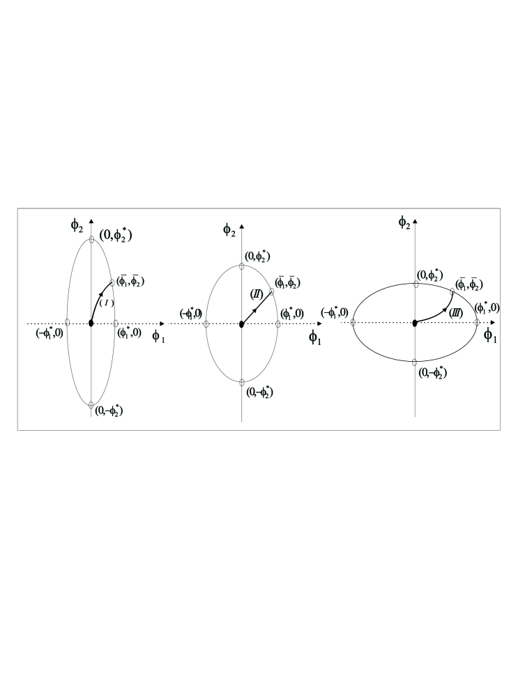
Figure 2: Phase space for $\mu_{1}/\mu_{2}=\lambda_{11}/\lambda_{12}$; $\lambda_{12}^{2}=\lambda_{11}\lambda_{22}$ showing orbits connecting the point $(0,0)$ to the coalesced ellipses. Orbit (I) is for $\lambda_{11}/\lambda_{22}>1$, (II) for $\lambda_{11}/\lambda_{22}=1$ and (III) is for $0<\lambda_{11}/\lambda_{22}<1$.

and the structure of the orbit depends strongly on the product $\lambda_{11}\lambda_{22}$, as shown in Fig. 2.

We now deal with the case of intersecting ellipses, which is depicted in Fig. 1(a). This case is very interesting, and it is better to refer to Fig. 3a, which shows the general configuration for the minimum energy points, where we defined $\phi_{12}\equiv\sqrt{\mu_{1}/\lambda_{12}}$ and $\phi_{21}\equiv\sqrt{\mu_{2}/\lambda_{21}}$.

To obtain the energies of the solutions connecting minima we first consider Eq. (9). We have, by symmetry, $W(\phi_{1},\phi_{2})=W(\phi_{1},-\phi_{2})=W(-\phi_{1},\phi_{2})$ $=W(-\phi_{1},-\phi_{2})$; thus, there are no kink-like structure connecting the intersecting points from the ellipses. Also, we have $W(\phi_{1}^{*},0)$ $=W(-\phi_{1}^{*},0)$ $=|\mu_{1}^{2}/(4\lambda_{11})|$ and $W(0,\phi_{2}^{*})$ $=W(0,-\phi_{2}^{*})=|\mu_{2}^{2}/(4\lambda_{22})|$. We studied the following cases:

i) One connection by means of a straight line between $(0,0)\rightarrow(0,\pm\phi_{2}^{*})$, with energy $E_{1}=|W(0,0|-W(0,\pm\phi_{2}^{*})|=|\mu_{2}^{2}/(4\lambda_{22})|$. This can be found solving the equations of motion to obtain

$$\phi_{1}(x)=0,\,\,\,\,\phi_{2}(x)=\pm\phi_{2}^{*}\left(\frac{1+\tanh{(\mu_{2}x)}}{2}\right)$$ (20)

This solution represents a laser operating only on mode 2, where the laser intensity smoothly increases from zero to the maximum operating value. By symmetry one can easily find similar solutions that connects $(0,0)\rightarrow(\pm\phi_{1}^{*},0)$ where the laser operates only on mode 1.

ii) We look for solutions that connect $(0,0)\rightarrow(\bar{\phi}_{1},\bar{\phi}_{2})$, with energy $E_{3}=|W(0,0|-W(\bar{\phi}_{1},\bar{\phi}_{2})|$. We try the orbit

$$\frac{\phi_{1}}{\bar{\phi}_{1}}=\biggl{(}\frac{\phi_{2}}{\bar{\phi}_{2}}\biggr{)}^{B}$$ (21)

Differentiating the orbit and substituting the first order equations leads to

$$\mu_{1}-\lambda_{11}\phi_{1}^{2}-\lambda_{12}\phi_{2}^{2}=B(\mu_{2}-\lambda_{21}\phi_{1}^{2}-\lambda_{22}\phi_{2}^{2})$$ (22)

Equating the independent coefficients we obtain $B={\mu_{1}}/{\mu_{2}}$ and the remaining condition can be written as

$$\biggl{(}\lambda_{11}-\frac{\mu_{1}}{\mu_{2}}\lambda_{21}\biggr{)}\phi_{1}^{2}=\biggl{(}\frac{\mu_{1}}{\mu_{2}}\lambda_{22}-\lambda_{12}\biggr{)}\phi_{2}^{2}$$ (23)

$$\bar{\phi}_{1}^{2}\det\Lambda^{(\phi_{2})}\biggl{(}\frac{\phi_{2}^{2}}{\bar{\phi}_{2}^{2}}\biggr{)}^{B}=\bar{\phi}_{2}^{2}\det\Lambda^{(\phi_{1})}\frac{\phi_{2}^{2}}{\bar{\phi}_{2}^{2}}$$ (24)

We then have the following possibilities:

$\bullet$ $\det\Lambda^{(\phi_{1})}=\det\Lambda^{(\phi_{2})}=0$. This leads to the already analyzed case of coalesced ellipses.

$\bullet$ $\det\Lambda^{(\phi_{1})},\,\det\Lambda^{(\phi_{2})}\neq 0$. This leads to $B=1$ and $\bar{\phi}_{1}^{2}\det\Lambda^{(\phi_{2})}=\bar{\phi}_{2}^{2}\det\Lambda^{(\phi_{1})}$, which means $\mu_{1}=\mu_{2}$ and $\lambda_{11}=\lambda_{22}\equiv\lambda$, respectively, with $\phi_{1}=\phi_{2}$. In this case one can obtain an expression for $\phi_{1}(x)$ by means of substituting the former equation into the equation of motion for the field $\phi_{1}$(cf. Eq.[10a]). One finds

$$\phi_{1}(x)=\phi_{2}(x)=\pm\sqrt{\frac{\mu}{\lambda_{12}+\lambda}\cdot\frac{1}{2}(1+\tanh(\mu x))}$$ (25)

One can see that for $x\rightarrow-\infty$, $(\phi_{1},\phi_{2})\to(0,0)$ and for $x\rightarrow+\infty$, $(\phi_{1},\phi_{2})\to(\pm\bar{\phi}_{1},\pm\bar{\phi}_{2})$. This corresponds to a laser operating is both modes with the same intensity, since we have for this solution $\phi_{1}(x)^{2}=\phi_{2}(x)^{2}$, which corresponds to $E_{1}(t)^{2}=E_{2}(t)^{2}=I(t)$. The intensity of the i-th mode increases continuously until achieving the maximum value given by $I_{max}={\mu}/{(\lambda_{12}+\lambda)}$.

iii) For the orbit $\phi_{1}=A\phi_{2}^{2}+B$ to connect $(\phi_{1}^{*},0)\to(0,\phi_{2}^{*})$, one must have $B=\sqrt{\mu_{1}/\lambda_{11}}=\phi_{1}^{*}$ and $A=-(\lambda_{22}/\mu_{2})\sqrt{(\mu_{1}/\lambda_{11})}$ $=-\phi_{1}^{*}/{\phi_{2}^{*}}^{2}$. Then we have the orbit

$$\frac{\phi_{1}}{\phi_{1}^{*}}+\biggl{(}\frac{\phi_{2}}{\phi_{2}^{*}}\biggr{)}^{2}=1$$ (26)

Deriving the orbit and using equations (10) leads to the consistency conditions

$$\lambda_{11}=2\lambda_{12},\,\,\,\,\frac{\lambda_{11}}{\lambda_{22}}=4+2\frac{\mu_{1}}{\mu_{2}}$$ (27)

We can show that conditions (27) are also compatible with the Eqs. (13) and (14) that define the intersecting points. Also, the condition for existence of the minimum energy points $(\bar{\phi}_{1},\bar{\phi}_{2})$ leads to another constraint on the parameters. We can see in Fig. 3(a) that crossing among the ellipses exist only if $\phi_{1}^{*}\geq\phi_{21}$ and $\phi_{2}^{*}\geq\phi_{12}$. This leads after using the consistency conditions to $2\leq\mu_{1}/\mu_{2}\leq 2+\mu_{1}/\mu_{2}$. This inequality is satisfied only when $\mu_{1}/\mu_{2}\geq 2$. When the ellipses do not cross one another, we must have, as one possibility, that $\phi_{1}^{*}\geq\phi_{21}$ and $\phi_{2}^{*}\leq\phi_{12}$. This, with the conditions (27) lead to the condition $\mu_{1}/\mu_{2}\geq 2+\mu_{1}/\mu_{2}$ which is an impossibility. So, this type of orbit needs the crossing among the ellipses. The phase space diagram for this orbit is shown on Fig. 3(b). There one shows that the points $(\pm\bar{\phi}_{1},\pm\phi_{2})$ are unstable. In this way the orbits connect one of these points, for $x\to-\infty$, to one of the other minimum energy points $(0,\pm\phi_{1}^{*})$ or $(\pm\phi_{2}^{*},0)$, for $x\to\infty$.

As an example we can choose $\lambda_{11}=3,\lambda_{22}=1/4,\mu_{1}=3,\mu_{2}=3/4$. This means a ratio $\mu_{1}/\mu_{2}=4\geq 2$ and $\lambda_{12}=\lambda_{11}/2=3/2$. This choice corresponds to an initial condition where mode 1 (represented by the $\phi_{1}$ field) is well above threshold, whereas mode 2 (corresponding to the $\phi_{2}$ field) has a smaller gain. We have minimum energy points $(\phi_{1}^{*},0)=(1,0)$, $(\bar{\phi}_{1},\pm\bar{\phi}_{2})=(1/2,\pm\sqrt{6}/2)$, $(0,\pm\phi_{2}^{*})=(0,\pm\sqrt{3})$ and an orbit $\phi_{1}=-(1/3)\phi_{2}^{2}+1$ connecting theses 6 points (three for $\phi_{2}\geq 0$ and three for $\phi_{2}\leq 0$). Substituting the orbit in Eq. (10a), we obtain

$$\frac{1}{\phi_{1}}\frac{d\phi_{1}}{dx}=-\frac{3}{2}(2\phi_{1}^{2}-3\phi_{1}+1)$$ (28)

Integrating the former equation we obtain two solutions that agree with $\phi_{2}\geq 0$, namely ($(\phi_{1}^{+}(x),\phi_{2}^{-}(x))$ and $(\phi_{1}^{-}(x),\phi_{2}^{+}(x))$, with:

$$\phi_{1}^{\pm}(x)=\frac{1}{2}\left(1\pm\sqrt{\frac{1}{2}(1+\tanh(3x/4)}\right)$$ (29)

and

$$\phi_{2}^{\mp}(x)=\sqrt{\frac{3}{2}\left(1\mp\sqrt{\frac{1}{2}(1+\tanh(3x/4)}\right)}$$ (30)

For $(\phi^{+}_{1}(x),\phi^{-}_{2}(x))$ we have $\lim_{x\to-\infty}\phi^{+}_{1}=1/2$, $\lim_{x\to-\infty}\phi^{-}_{2}=\sqrt{6}/2$ and $\lim_{x\to+\infty}\phi^{+}_{1}=1$, $\lim_{x\to+\infty}\phi^{-}_{2}=0$ and the orbit connects $(\bar{\phi}_{1},\bar{\phi}_{2})\rightarrow(\phi_{1}^{*},0)$ as $(1/2,\sqrt{6}/2)\rightarrow(1,0)$. Here we have a final state where only mode 1 oscillates. In this regime we can say that oscillation in mode 2 was quenched nuss by the oscillation in mode 1. For $(\phi^{-}_{1}(x),\phi^{+}_{2}(x))$ we have $\lim_{x\to-\infty}\phi^{-}_{1}=1/2,\lim_{x\to-\infty}\phi^{+}_{2}=\sqrt{6}/2$ and $\lim_{x\to+\infty}\phi^{-}_{1}=0,\lim_{x\to+\infty}\phi^{+}_{2}=\sqrt{3}$, and the orbit connects $(\bar{\phi}_{1},\bar{\phi}_{2})\rightarrow(0,\phi_{2}^{*})$ as $(1/2,\sqrt{6}/2)\rightarrow(0,\sqrt{3}).$ Now we have the opposite regime, where mode 2 absorbs energy continuously and mode 1 decreases until only mode 2 remains.

In conclusion, in this work we have used the trial orbit method introduced by Rajaraman t4 to investigate first order differential equations which appear when one uses the Bogomol’nyi approach to study minima energy kink-like solutions bog . We have studied a family of models described by two real scalar fields inspired on the theory of two-mode laser. We have determined all the minimum energy points in terms of the parameters which specify the model. We have found a rich structure of minima, and several analytical solutions of the kink-like type, connecting pairs of minima in the field space. In order to correctly map our results for $\phi_{1}(x)$ and $\phi_{2}(x)$ to the time-dependent problem of the dynamical competition between the two modes $E_{1}(t)$ and $E_{2}(t)$, we must interpret $x$ from our mathematical solutions as the physical time $t$. This is justifiable after comparing Eqs. (10a)-(10b) from our classical field theory with Eq. (10c) from the semiclassical laser theory. In this way some of the exact solutions here studied where used to study phenomenological situations such as laser oscillations between two modes in a multi-mode system.

The authors would like to thank CAPES, CNPq, MCT-CNPq-FAPESQ and MCT-CNPq-CT-Infra for partial support. The authors also thank C. Furtado for discussions and M. M. Ferreira Jr. for reading the manuscript.

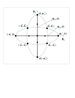
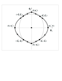
Figure 3: (a) Phase space for $\mu_{1}/\lambda_{12},\mu_{2}/\lambda_{21}>0;$ $\mu_{1}/\lambda_{11},\mu_{2}/\lambda_{22}>0$ showing the 9 minimum energy points - 4 of them obtained by the intersection points of the ellipses - and some orbits. (b) Phase space for $\lambda_{11}=2\lambda_{12}$ and $\lambda_{11}/\lambda_{22}=4+\mu_{1}/\mu_{2}$, showing the orbits $\phi_{1}=\pm\phi_{1}^{*}(-{\phi_{2}^{2}}/{{\phi_{2}^{*}}^{2}}+1).$

References

(1) R. Rajaraman, Solitons and Instantons. An introduction to
solitons and instantons in quantum field theory (Elsevier, Amsterdam, 1982).
(2) N. Manton and P. Sutcliffe, Topological Solitons (Cambridge Univ. Press,
Cambridge, UK, 2004).
(3) V. Rubakov, Classical theory of gauge fields (Princeton Univ. Press,
Princeton, 2002).
(4) R. Rajaraman and E. J. Weinberg, Phys. Rev. D 11, (1975), 2950.
(5) C. Montonen, Nucl.
Phys. B 112, (1976), 349.
(6) S. Sarker, S. E. Trullinger, A. R. Bishop, Phys. Lett. A 4, (1976), 255.
(7) R. Rajaraman, Phys. Rev. Lett. 42, (1979), 200.
(8) E. Magyari and H. Thomas, Phys. Lett. A 100, (1984), 11.
(9) H. Ito, Phys. Lett. A 112, (1985), 119.
(10) E. B. Bogomol’nyi, Sov.
Journ. Nucl. Phys. 24, (1976), 449.
(11) D. Bazeia, M. J. dos Santos, R. F. Ribeiro, Phys. Lett. A 208, (1995), 84.
(12) D. Bazeia, F. A. Brito, Phys. Rev. D 61, (2000), 105019.
(13) D. Bazeia, W. Freire, L. Losano and R. F. Ribeiro, Mod. Phys. Lett. A
17, (2002), 1945.
(14) A. Alonso Izquierdo, M.A. Gonzalez Leon, J. Mateos Guilarte, M. de la Torre Mayado, Phys.Rev. D 66, 105022 (2002).
(15) A. Alonso Izquierdo, M.A. Gonzalez Leon, M. de la Torre Mayado, J. Mateos Guilarte, Physica D 200, 220 (2005).
(16) A. Alonso Izquierdo, J. Mateos Guilarte, Physica D 220, 31 (2006).
(17) M. A. Shifman and M. B. Voloshin, Phys. Rev. D 57 (1998) 2590.
(18) A. Alonso Izquierdo, M.A. Gonzalez Leon, J. Mateos Guilarte, Phys.Rev. D 65, 085012 (2002).
(19) M. Eto and N. Sakai, Phys. Rev. D 68 (2003) 125001.
(20) A. de Souza Doutra, Phys. Lett. B 626 (2005) 249.
(21) M. Giovannini, Phys. Rev. D 74 (2006) 087505 and 75 (2007) 064023.
(22) H. M. Nussenzveig Introduction to Quantum Optics ( Gordon and Breach, New York, 1973).